www.scielo.br/rbg
SPATIAL AND TEMPORAL CHARACTERISTICS OF OUTGOING
LONGWAVE RADIATION (OLR): AN UPDATE
Rajaram Purushottam Kane
Recebido em 2 marc¸o, 2007 / Aceito em 2 junho, 2008 Received on March 2, 2007 / Accepted on June 2, 2008
ABSTRACT.A study of the Outgoing longwave radiation (OLR) values (Unit, W/m2) observed by various satellites during 1979-2002 revealed that the OLR values varied considerably from one geographical region to another (∼100-300 units). The climatology was latitude dependent. At middle and high latitudes, the range (minimum to maximum) was∼40-60 units, with maximum in local summer and minimum in local winter, but at lower latitudes, the range reduced considerably and was uncertain near equator. Near equator, the long-term changes (as seen in 12-month moving averages) were: OLR decreases during ENSO events in the eastern Pacific up to the dateline, and OLR increases during ENSO events in the Australasian region. Outside the equatorial region, the OLR changes were small during ENSO events and negligible in other years. In some longitudes at middle and high latitudes, the OLR changes occurred several months after the El Ni ˜no events, coinciding with La Ni˜na (cold water events, opposite of warm water El Ni˜no events).
Keywords: spectra, OLR (Outgoing Longwave Radiation).
RESUMO.Um estudo dos valores (em unidades de W/m2) da emiss˜ao de radiac¸˜ao de ondas longas (OLR) observados por sensores em v´arios sat´elites entre 1979 e 2002 revelou que os valores de OLR variavam consideravelmente de uma regi˜ao geogr´afica para outra (∼100-300 unidades). A climatologia era dependente da latitude. Em latitudes medias e altas, a faixa de variac¸˜ao (m´ınima e m´axima) era de∼40-60 unidades, com valores m´aximos no ver˜ao local e m´ınimos no inverno, por´em, em baixas latitudes, a faixa se tornava consideravelmente reduzida e oscilante pr´oximo do equador. Neste caso, as mudanc¸as de longo termo (como observado em m´edias m´oveis de 12 meses) eram: os valores de OLR decresciam at´e odateline durante os eventos ENSO do Pac´ıfico oriental e aumentavam durante os eventos ENSO na regi˜ao da Austr´alia. Fora da regi˜ao equatorial, as mudanc¸as do OLR eram pequenas durante os eventos ENSO e insignificante nos outros anos. Em algumas longitudes, em latitudes m´edias e altas, as mudanc¸as OLR ocorreram em diversos meses ap´os os eventos El Ni˜no, coincidindo com La Ni˜na (eventos de ´aguas frias, opostos aos de ´aguas quentes dos eventos El Ni˜no).
Palavras-chave: spectra, OLR (Outgoing Longwave Radiation).
Instituto Nacional de Pesquisas Espaciais, P.O. Box 515, 12245-970 S˜ao Jos´e dos Campos, SP, Brazil. Phone: +55 (12) 3945-6795; Fax: +55 (12) 3945-6810
228
CHARACTERISTICS OF OUTGOING LONGWAVE RADIATION (OLR)INTRODUCTION
Terrestrial energy budget is mainly governed by the incoming Total Solar Irradiance (TSI) and the Outgoing Longwave Radi-ation (OLR). Among these, TSI is almost constant (often cal-led ‘Solar Constant’). Hence the variations of terrestrial weather and climate should have a considerable contribution from the space and time variations of OLR. The studies of OLR prior to the advent of satellites are reviewed by Hunt et al. (1986). A his-tory of satellite missions and measurements of the Earth’s radi-ation budget during 1957-1984 has been traced by House et al. (1986). Winston et al. (1979) used the scanning radiometer (SR) aboard operational meteorological satellites to compute OLR and published a data set for June 1974-March 1978. Heddinghaus & Krueger (1981) subjected this data set to an Empirical Orthogo-nal Function (EOF) aOrthogo-nalysis and determined the annual and semi-annual cycles and intersemi-annual variations for that period. Bess et al. (1992) used EOF approach on a 10-year data set, found that the first EOF accounted for 66% of the variance, the first two EOFs described mainly the annual cycle, the third EOF descri-bed mainly the semiannual cycle, and the fourth EOF descridescri-bed much of the 1976-1977 and 1982-1983 El Ni˜no/Southern Os-cillation (ENSO) phenomena (besides other details). Chelliah & Arkin (1992) used OLR data derived from NOAA’s polar-orbiting satellites for more than 15 years, performed a Rotated Principal Component Analysis (RPCA) on monthly OLR anomalies over the global tropics (30◦N-30◦S) on a 10◦ longitude by 5◦ latitude grid for June 1974-March 1989, excluding calendar year 1978. The spatial-loading pattern and the time series for the first prin-cipal component (first RPC), the ‘canonical ENSO mode’, repre-sented the major large-scale features in the tropics during the typical phase of the major warm (El Ni˜no) and cold (La Ni˜na) events in the tropical Pacific during the analysis period. How-ever, the characteristics of the dramatic 1982-1983 warm event (El Ni˜no) were different from the canonical ENSO mode and com-pletely dominated the second RPC. (The third and fourth leading RPCs described the changes in the satellite-observing system). Barnett & Preisendorfer (1978) have attempted multifield analog predictions of short-term climate fluctuations using a climate state vector. For the tropical regions, several workers have used OLR as indicators of annual, interannual and interseasonal variability of convective activity. Liebmann & Hartmann (1982) studied the interannual variations of OLR associated with tropical circulation changes during 1974-1978. Kousky (1988) studied OLR clima-tology for the South American sector. Ferreira & Gurgel (2002) studied the annual and interannual variability of OLR above South
America and its vicinity. Kayano et al. (1995) studied the OLR biases and their impacts on EOF modes of interannual variability in the tropics.
In the present communication, OLR data are used for 1974-2002 (omitting 1978) to illustrate the geographical distribution, climatology, and long-term variations of OLR during this interval, and in particular, to obtain theirspectra.
DATA
OLR data were available on several websites, for example, http://ingrid.ldeo.columbia.edu/maproom/.Global/.Precipitation/ Monthly OLR.html, http://ingrid.ldeo.columbia.edu/SOURCES/ .NOAA/.NCEP/.CPC/.GLOBAL/.monthly/.olr/, http://tao.atmos. washington.edu/data sets/olr/index.html, in a 2.5◦×2.5◦ grid in different formats and were accessed as needed for different purposes.
PLOTS
Geographical distribution
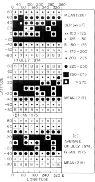
Figure 1 shows a plot of the absolute OLR values (W/m2) in a 10◦×10◦grid, latitudes top to bottom (North to South), longitu-des left to right (0-360 E, or 360W-0), for (a) July 1974 (northern summer) in the upper half and (b) January 1975 (northern winter) in the lower half. The OLR values in different ranges are indica-ted by symbols (100-125, xx; 125-150, x; 150-175, B; 175-200, small open circle; 200-225, small full circle; 225-250, big full circle; 250-275, full square;>275 full square with an open cir-cle in the center). The average value is∼220 and small full cir-cles (200-225) would represent average values. (There was no El Ni˜no event during 1974-1975, only later in 1976-1977). The following may be noted:
(1) The summer and winter values are very different at very high latitudes (near the poles). The winter values (xx) are almost half of the summer values (small full circles). This is because the OLR is associated with surface tempera-ture and clouds and the levels of surface temperatempera-ture and cloud cover are very different in summer and winter. In the tropics, the seasonal variability also depends on the pre-sence or abpre-sence of convective activity.
con-Figure 1– OLR (Outgoing longwave radiation) monthly values (W/m2) in different ranges (shown by different symbols) for a 10◦×10◦grid, for (a) July 1974 (upper part) and (b) January 1975 (lower part).
vection are found over the equatorial land masses, Ama-zon basin, and in the western equatorial Pacific. OLR
<200 Wm-2are also associated with the cold tempera-tures of the Himalayas. High annual mean OLR values (>280 Wm-2) are observed over the central and
230
CHARACTERISTICS OF OUTGOING LONGWAVE RADIATION (OLR)seen over western equatorial Pacific also (5◦N-5◦S, 120◦ -150◦W). (This pattern for 1974-1975 may not be exactly so in other years, but will probably be roughly valid).
If values are averaged over wider ranges, the pattern looks as shown in Figure 2, for a 20◦latitude by 40◦longitude grid, for July 1974 in the upper part (overall mean OLR value 226), June 1975 in the middle (overall mean OLR value 213), and their average in the lower part (overall mean OLR value 219). In the average, the south pole region has values below average. Values above average are in the 50◦N-50◦S belt, more so in the 30◦N-30◦S belt, with values varying in a large range (200-275) at different longitudes.
Figure 2– OLR values in different ranges (shown by different symbols) for a 20◦latitude×40◦longitude grid, for (a) July 1974 (upper part) and (b) January 1975 (middle part), (c) Average of July 1974 and January 1975 (lower part).
Climatology
The climatology (values for January, February, etc., averaged over several years) is shown in Figure 3, for 60◦longitude ranges in successive columns. The following may be noted:
(1) The month-to-month pattern is basically annual, with max-imum in summer (July-August in northern hemisphere, December-January in southern hemisphere) and minimum in winter, particularly conspicuous at middle and high latitudes.
(2) The ranges (minimum to maximum) are about the same at very high latitudes (50-60 OLR units), but reduce at lower latitudes, faster in the southern hemisphere.
(3) In low latitudes, the climatology is obscure. The maxima are diffuse and not necessarily in mid-summer. This might have resulted in the semiannual component mentioned by Bess et al. (1992).
However, it may be noted that the latitude range of 22.5◦ chosen here may be too large and may be obliterating changes in finer latitude ranges. It is well known that in parts of the tropics, OLR values are smaller in the summer hemisphere (May-August in the northern hemisphere, November-February in the southern hemisphere) due to convective clouds (cloud tops with low tem-peratures). In these regions, OLR values are higher in the win-ter hemisphere due to the absence of convection. In contrast, in middle and high latitudes, winter values of OLR are low due to lower surface temperature, not due to cloud cover.
Long-term variation
Even though deseasoned monthly anomaly values were available, these were sometimes erratic. Hence, further 12-month moving averages calculated. There was a gap in data for several months in 1978. Hence, only data for 1979 onwards are considered. Figure 4 shows the plot of 12-month moving averages (running means) centered 3 months apart (4 values per year) for the equat-orial region (5◦N-5◦S). The top plots are for the well-known phenomenon ENSO, which is briefly as follows.
Figure 3– Climatology (values for Jan., Feb.,. . .Dec., each averaged over 1974-2002) for northern and southern latitudes centered at 85◦, 67.5◦, 45◦, 22.5◦, 0◦, and longitude ranges 0◦-60◦, 60◦-120◦,. . .300◦-360◦. Circled numbers are OLR ranges (W/m2, minimum to maximum). The maxima are indicated by dots.
temperature and rainfall along and near the Peru-Ecuador coast, defining intensities based on the positive sea-surface tempera-ture anomalies along the coast as: Strong, in excess of 3◦C; Moderate, 2.0◦-3.0◦C; Weak, 1.0◦-2.0◦C. The warming at the coast extends to farther regions of the Pacific to the west of Peru-Ecuador. Monthly SST (sea surface temperature) anom-alies are available on the Climate Prediction Center website http://www.cpc.ncep.noaa.gov/data/indices/, for regions Ni˜no 1+2 (0-10◦S, 90◦-80◦W), Ni˜no 3 (5◦N-5◦S, 150◦-90◦W), Ni˜no 3.4 (5◦N-5◦S, 170◦-120◦W), Ni˜no 4 (5◦N-5◦S, 160◦E-150◦W).
A phenomenon intimately related to the El Ni˜no occurrence is the Southern Oscillation (SO). It is a global pattern of short-term climatic fluctuations with a characteristic period of 2-7 years (e.g., Trenberth, 1997). A SO index can be simply represented by the Tahiti T (18◦S, 150◦W) minus Darwin D (12◦S, 131◦E) mean sea level pressure difference (T-D). Normally, the pressure at Tahiti is higher than that at Darwin by a few millibars. However, this pressure difference fluctuates (like a seesaw), sometimes re-duces to zero (or becomes even negative) and this reduction is often associated with the occurrence of El Ni˜nos. In Figure 4, the top plot is for SST anomalies in the Ni˜no 1+2 region. The posit-ive anomalies are painted black and show the prominent El Ni˜nos of 1982-1983 (strong), 1986-1987 (moderate), 1991-1994 (weak and diffuse), and 1997-1998 (very strong). The next plot is for (T-D), (data from Parker, 1983, and the Climate Prediction Center website http://www.cpc.ncep.noaa.gov/data/indices/). The posit-ive anomalies are painted black, negatposit-ive anomalies are shown
hatched, and these match very well with the negative anomalies and positive anomalies of SST (anticorrelation). Interestingly, during 1991-1994, SST anomalies are not large and are not uni-form over the whole period, but (T-D) is consistently negative over the whole period, indicating that SST and (T-D) could have different evolutions.
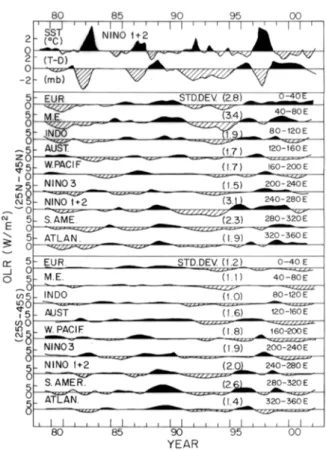
The succeeding nine plots in Figure 4 are for OLR anomalies at longitudes 0-40◦E, 40◦-80◦E, and 320◦-360◦E. The tenth plot is for their average. The standard deviations of the OLR series are indicated. The following may be noted:
(1) The series for 160◦-200◦E (160◦E-160◦W, through date-line 180◦, western Pacific, almost the same as Ni˜no 4), has the largest standard deviation (12.9 units) and shows prominent decreases of OLR during the El Ni˜no events.
(2) The effect is also seen (slightly reduced standard devia-tion, 10.4) in the next longitude range 200◦-240◦E (160◦ -120◦W, almost Ni˜no 3.4), and still more reduced in 240◦ -280◦E (5.6 units) (120◦-80◦W, almost Ni˜no 3). Thus, the OLR of the whole Pacific responds (shows decreases) during El Ni˜no events.
(3) On the other side, the longitude range 120◦-160◦E (Aus-tralasia) has a considerable standard deviation (6.0), but the effects are opposite, namely, increases of OLR ins-tead of decreases. This positive effect is also seen in 80◦ -120◦E (Indonesia).
232
CHARACTERISTICS OF OUTGOING LONGWAVE RADIATION (OLR)Figure 4– Plots of 12-month moving averages centered 3 months apart (4 values per year), for 1979-2002. Top plot is for SST (sea surface tempera-ture) anomalies in the Ni˜no 1+2 region (0-10◦S, 90◦-80◦W), and the next plot is for (T-D) (Tahiti minus Darwin atmospheric pressure difference, an in-dex of Southern Oscillation). Positive anomalies are painted black and nega-tive anomalies are shown hatched. The other plots are for OLR in the equato-rial latitudes (5◦N-5◦S), for nine longitude ranges 0◦-40◦, 40◦-60◦,. . .320◦ -360◦, and their average (bottom plot). Numbers in parentheses are standard deviations of the series.
Thus, El Ni˜no effects are mostly confined to the Pacific. In the websitehttp://tao.atmos.washington.edu/data sets/olr/index.html, Todd Mitchell mentions, “The regions of large OLR variance (>10 Wm-2) are over a broad region of the Indian and Pacific Oceans with largest values (>20 Wm-2) on and slightly to the south of the equator in the western Pacific”, which is roughly cor-rect. Todd Mitchell also mentions, “Warm equatorial Pacific SST anomalies are associated with below normal OLR (enhanced deep atmospheric convection) between 165◦E and the Ecuador coast in the equatorial Pacific, and enhanced OLR (diminished convective rainfall) over Papua New Guinea and eastern equatorial Brazil”.
Figure 5 shows similar plots for the low latitude ranges 5◦ N-25◦N, followed by 5◦S-25◦S, each for nine longitude ranges. Only 80◦-120◦E (5.0 units), 120◦-160◦E (6.0 units), 160◦-200◦E (5.1 units) in the northern hemisphere and 120◦-160◦E (4.1 units) in the southern hemisphere show substantial standard deviations, and the effects seem to be positive (OLR increases), in some cases with a lag of one year. Effects at other longitudes are small. Note that the vertical scale in Figure 5 is expanded double as compared to Figure 4.
Figure 5– Plots of 12-month moving averages centered 3 months apart (4 values per year), for 1979-2002. Top plot is for SST (sea surface temperature) anomalies in the Ni˜no 1+2 region (0-10◦S, 90◦-80◦W), and the next plot is for (T-D) (Tahiti minus Darwin atmospheric pressure difference, an index of Southern Oscillation). Positive anomalies are painted black and negative anomalies are shown hatched. The other plots are for OLR in the low latitude ranges (5◦ N-25◦N, and 5◦S-25◦S), for nine longitude ranges 0◦-40◦, 40◦-60◦,. . .320◦ -360◦. Numbers in parentheses are standard deviations of the series.
Figure 6 shows similar plots for the middle latitude ranges 25◦N-45◦N, followed by 25◦S-45◦S, each for nine longitude ran-ges. The vertical scale is expanded double as compared to Fig-ure 5. All the standard deviations are small (less than 4.0, often less than 2.0). Some positive anomalies match with SST anoma-lies but most of them do not match. Interestingly, during 1991-1994, OLR anomalies are consistently negative (like T-D) at al-most all longitudes. Also, some anomalies are large about an year after an El Ni˜no. Since this interval is often a La Ni˜na event (cold water events, negative SST anomalies opposite to El Ni˜no, positive T-D anomalies), it is likely that OLR anomalies outside the equatorial regions are related to La Ni˜nas.
(painted black) or negative (shown hatched) OLR anomalies seem to be in years following an El Ni˜no (La Ni˜na years).
Figure 6– Same as Figure 5, for middle latitude ranges (25◦N-45◦N, and 25◦S-45◦S).
Figure 8 shows similar plots for the auroral and polar latitude ranges 65◦N-85◦N, followed by 65◦S-85◦S, each for nine longit-ude ranges. The vertical scale is the same as in Figure 6. All the standard deviations are small (less than 2.1). Most of the large positive (painted black) or negative (shown hatched) OLR anom-alies seem to be in years following an El Ni˜no (La Ni˜na years).
It would thus seem that El Ni˜no relationship is seen clearly only in the equatorial latitudes, while outside, the magnitudes are small and the relationship is delayed and coincides with the suc-ceeding La Ni˜na year. As will be illustrated in the next section, the OLR variations have spectra similar to those of surface tem-perature, and since OLR is intimately related to surface tempera-ture, the OLR variations are directly related to surface temperature variations.
SPECTRA
If there is a strong relationship between OLR and ENSO, their spectra should tally completely. To obtain quantitative estima-tes of the characteristics of the interannual variability, the series
were subjected to spectral analysis. The method used was MEM (Maximum Entropy Method, Burg, 1967; Ulrych & Bishop, 1975), which locates peaks much more accurately than the conventional BT (Blackman & Tukey, 1958) method. However, the amplitude (Power) estimates in MEM are not very reliable (Kane, 1977, 1979; Kane & Trivedi, 1982). Hence, MEM was used only for detecting all the possible peaksTk(k=1 to n), using LPEF (Length of the Prediction Error Filter) as 50% of the data length. TheseTkwere then used in the expression:
f(t)=Ao+ n
k=1
aksin 2π
t Tk
+bkcos 2π
t Tk
+E
=Ao+ n
k=1
rksin(2πt/Tk+φk)+E
wheref(t)is the observed series andEthe error factor. A Multi-ple Regression Analysis (MRA, Bevington, 1969) was then carried out to estimateAo,ak,bk, and their standard errors (by a least-square fit). From these, amplitudesrk and their standard error
σk(common for allrkin this methodology, which assumes white noise) were calculated. Anyrk exceeding2σ is significant at a 95% (a priori) confidence level.
234
CHARACTERISTICS OF OUTGOING LONGWAVE RADIATION (OLR)Figure 8– Same as Figure 5, for auroral and polar latitude ranges (65◦N-85◦N, and 65◦S-85◦S).
Figure 9 shows the spectra (amplitudesversusperiodicities). The abscissa scale is log(T). The hatched portions indicate the 2σ limit and lines protrouding above this area are significant at a better than 95% (a priori) confidence level. The top plot is for SST of Ni˜no 1+2 region. The most prominent periodicity is T=5.1 years. The next prominent ones are T=3.6 and 8.1 years. There are some QBOs (Quasi-biennial oscillations) of 2.06 and 2.76 year periodicity, barely significant. The next plot is for the Southern Oscillation index (T-D). The periodicities are almost the same as for SST, but not quite. MEM is very, very accurate in periodicity determination. As shown in Kane (1977, 1979), spec-tra of artificial samples show that the accuracy near 2.00 years is better than±0.03 years, and at 5.00 years, better than±0.05 years. Hence T=2.06 and 3.6 years of SST may be considered as the same as T=2.09 and 3.7 years of (T-D), but T=2.76, 5.1, 8.1 years of SST are definitely different from T=2.50, 5.4, 10.9 years of (T-D), showing that Pacific SST and the seesaw of (T-D) may have slightly different evolutions. This was seen glaringly in the top plots of Figure 4 where for 1991-1994, SST in Ni˜no 1+2 region had a small, erratic (intermittent) evolution while (T-D) had a consistent negative anomaly.
Figure 9– Spectra (amplitudesversus periodicities T) for series 1979-2002. The numbers are periodicities T (in years) obtained by MEM (Maximum Entropy Method). The top plot is for SST (Ni˜no 1+2), the next for (T-D), and the others are for equatorial OLR (5◦N-5◦S), for nine longitude ranges 0◦-40◦, 40◦-60◦, . . . 320◦-360◦. The abscissa scale is logT.
The other plots in Figure 9 are for equatorial (5◦N-5◦S) OLR in 0-40◦E, 40◦-80◦E, 320◦-360◦E longitude belts (series plotted in Fig. 4). The following may be noted:
(1) The periodicities marked with rectangles (T=2.06-2.09, 2.50, 3.5-3.7, 5.3-5.4 years) are common to (T-D) and some OLR series, notably OLR (160◦-200◦E).
(2) The periodicities marked with a circle (T=4.8-5.1 years) are common to SST and some OLR series.
0-40◦, 80◦-120◦, 120◦-160◦, 160◦-200◦, 320◦-360◦E. In longitudes 200◦-320◦E (40◦-160◦W, eastern and mid-dle Pacific), T=∼3.6 years is conspicuous by its absence and only T=4.8-5.0 years is prominent.
(4) The T=8.1 year periodicity of SST is roughly seen in longitudes 200◦-320◦E, while T=10.9 years (sunspot cycle?) of (T-D) is seen only in 160◦-200◦E.
(5) The T=1.70 year (20 months) signal of (T-D) (barely sig-nificant) is seen in some OLR series (barely sigsig-nificant). On the other hand, signals at∼1.50 and∼1.84 years (18 and 22 months) are seen in some OLR series but not in SST or (T-D).
Almost all these series in the 5◦N-5◦S latitude belt had large standard deviations (exceeding 3.0 OLR units). For other latit-udes, the standard deviations were smaller and the spectra would not be reliable. Nevertheless, some series like 25◦-45◦S, 280◦ -320◦E (standard deviation 2.6, Figure 6, second plot from bot-tom) were subjected to spectral analysis and showed prominent periodicities at T=3.5 and∼6.0 years, while some others like 65◦-85◦S, 40◦-80◦E (standard deviation 2.0, Figure 8, eighth plot from bottom) showed only a prominent periodicity at T=∼7.0 years. Thus, there was partial or full matching with the ENSO signal.
In this connection, the spectra of temperature series would be of great relevance. Kane & Buriti (1997) subjected temperature value series at different altitudes (including surface) and latitudes. For higher altitudes, the spectra matched with the stratospheric low latitude zonal winds particularly for the tropics. For low alti-tudes, including surface, periodicities observed were very similar to those obtained here. Hence, the relationship between OLR and surface temperatures is valid even for spectra.
CONCLUSIONS
A study of the Outgoing Longwave Radiation (OLR) values (Unit W/m2) observed by various satellites during 1979-2002 revealed the following characteristics:
(1) The OLR values varied considerably from one geographi-cal region to another (∼100-300 units), probably due to a variety of Earth surfaces (landmasses with different or no vegetations, snow covers, sea surface, etc.) also, but mainly due to differences in the surface temperatures and local cloud covers.
(2) The climatology was latitude dependent. At middle and high latitudes, the range (minimum to maximum) was ∼40-60 units, with maximum in local summer and
min-imum in local winter, but at lower latitudes, the range re-duced considerably and was uncertain near equator.
(3) Near equator, the long-term changes (as seen in 12-month moving averages) were: OLR decreases during ENSO events in the eastern Pacific up to the dateline, and OLR increases during ENSO events in the Australasian region. Outside the equatorial region, the OLR changes were small during ENSO events and negligible in other years. In some longitudes at middle and high latitudes, the OLR changes occurred several months after the El Ni˜no events, coinci-ding with La Ni˜na (cold water events, opposite of warm water El Ni˜no events), which generally follow El Ni˜nos. All these should be related to convection in the Pacific, local circulations and to the generation mechanisms of El Ni˜nos and La Ni˜nas.
(4) A spectral analysis of OLR series indicated periodicities of 3.6, 5.1, 8.1 years etc. These are similar to the periodicities in low altitude (including surface) of atmospheric tempera-tures as described in Kane & Buriti (1997). Thus, all OLR characteristics including spectra are related to surface tem-peratures as expected, because physically, OLR intensity depends upon surface temperatures, besides cloud cover.
In some cases, small long-term trends were noticed, but were not studied further as Tashima & Hartmann (1999) have reported that such trends in ORL (for example, observed by the Nimbus-7 satellite during 1979-1987) were mostlyinstrumentalin nature.
ACKNOWLEDGMENTS
Thanks are due to various workers who were involved in obtai-ning the OLR data and to those who presented the data in seve-ral websites, notably NCEP (Washington, DC) and NOAA-CIRES (Boulder, Colorado). Thanks are due to Todd Mitchell for very valuable suggestions and to Vaman Kulkarni and Arcilan Assireu for computational assistance. Thanks are due to the refe-rees for valuable suggestions. This work was partially supported by FNDCT, Brazil under contract FINEP-537/CT.
REFERENCES
236
CHARACTERISTICS OF OUTGOING LONGWAVE RADIATION (OLR)BESS TD, SMITH GL, CHARLOCK TP & ROSE FG. 1992. Annual and interannual variations of Earth-Radiation based on a 10-year data set. J. Geophys. Res., 97: 12825–12835.
BEVINGTON PR. 1969. Data Reduction and Error Analysis for the Phys-ical Sciences. McGraw-Hill, New York, pp. 164–176.
BLACKMAN RB & TUKEY JW. 1958. The Measurement of Power Spectra. Dover, New York, 190 pp.
BURG JP. 1967. Maximum Entropy Spectral Analysis, paper presented at the 37th Meeting. Society of Exploration Geophysics, Oklahoma City, October.
CHELLIAH M & ARKIN P. 1992. Large-scale interannual variability of monthly outgoing longwave radiation anomalies over the global tropics. J. Climate, 5: 371–389.
FERREIRA NJ & GURGEL H de C. 2002. Variabilidade dos ciclos anual e interanual da radiac¸˜ao de ondas longas emergentes sobre a Am´erica do Sul e vizinhanc¸as. Rev. Brasileira de Engenharia Agr´ıcola e Ambiental, 6: 440–444.
HEDDINGHAUS TR & KRUEGER AF. 1981. Annual and interannual vari-ations in outgoing longwave radiation over the tropics. Mon. Wea. Rev., 109: 1208–1218.
HOUSE FB, GRUBER A, HUNT GE & MECHERIKUNNEL AT. 1986. History of satellite missions and measurements of the Earth’s radiation budget (1957-1984). Rev. Geophys., 24: 357–377.
HUNT GE, KANDEL R & MECHERIKUNNEL AT. 1986. A history of pre-satellite investigations of the Earth’s radiation budget. Rev. Geophys., 24: 351–356.
KANE RP. 1977. Power spectrum analysis of solar and geophysical parameters. J. Geomag. Geoelect., 29: 471–495.
KANE RP. 1979. Maximum Entropy Spectral Analysis of some artificial samples. J. Geophys. Res., 84: 965–966.
KANE RP & BURITI RA. 1997. Latitude and altitude dependence of the interannual variability and trends of atmospheric temperatures. Pure and Applied Geophysics, 149: 775–792.
KANE RP & TRIVEDI NB. 1982. Comparison of maximum entropy spec-tral analysis (MESA) and least-square linear prediction (LSLP) methods for some artificial samples. Geophysics, 47: 1731–1736.
KAYANO MT, KOUSKY VE & JANOWIAK JE. 1995. Outgoing longwave radiation biases and their impacts on Empirical Orthogonal function modes of interannual variability in the tropics. J. Geophys. Res. (Atmo-spheres), 100(D2): 3173–3180.
KOUSKY VE. 1988. Pentad outgoing longwave radiation climatology for the South American sector. Rev. Brasileira de Meteorologia, 3: 217–231.
LIEBMANN B & HARTMANN DL. 1982. Interannual variations of out-going IR associated with tropical circulation changes during 1974-78. J. Atmos. Sci., 39: 1153–1162.
PARKER DE. 1983. Documentation of a southern oscillation index. Meteorol. Mag., 112: 184–188.
QUINN WH, ZOPF DG, SHORT KS & KUO YANG RTW. 1978. Historical trends and statistics of the Southern Oscillation, El Ni˜no, and Indonesian droughts. Fish. Bull. (USA), 76: 663–678.
QUINN WH, NEAL VT & ANTUNEZ DE MAYOLO SE. 1987. El Ni˜no occurrences over the past four and a half centuries. J. Geophys. Res., 92: 14449–14461.
TASHIMA DH & HARTMANN DL. 1999. Regional trends in Nimbus-7 OLR: Effects of a spectrally nonuniform albedo. J. Climate, 12: 1458– 1466.
TRENBERTH KE. 1997. The definition of El Ni˜no. Bull. Amer. Meteor. Soc., 78: 2771–2777.
ULRYCH TJ & BISHOP TN. 1975. Maximum Entropy Spectral Analysis and autoregressive decomposition. Rev. Geophys., 13: 183–200.
WINSTON JS, GRUBER A, GRAY JR TI, VARNADORE MS, EARNEST CL & MANELLO NP. 1979. Earth-atmosphere radiation budget analysis derived from NOAA satellite data, June 1974-February 1978, vols. 1 and 2, NOAA S/T 79-187. Natl. Oceanic and Atmos. Admin. Washington, D.C.
NOTE ABOUT THE AUTHOR