EXTRACTION OF SOIL WATER BY PLANTS:
DEVELOPMENT AND VALIDATION OF A MODEL
(1)Q. de JONG van LIER(2) & P. L. LIBARDI(3)
SUMMARY
A quantitative model of water movement within the immediate vicinity of an individual root is developed and results of an experiment to validate the model are presented. The model is based on the assumption that the amount of water transpired by a plant in a certain period is replaced by an equal volume entering its root system during the same time. The model is based on the Darcy-Buckingham equation to calculate the soil water matric potential at any distance from a plant root as a function of parameters related to crop, soil and atmospheric conditions. The model output is compared against measurements of soil water depletion by rice roots monitored using γγγγγ-beam attenuation in a greenhouse of the Escola Superior de Agricultura “Luiz de Queiroz”/Universidade de São Paulo(ESALQ/USP) in Piracicaba, State of São Paulo, Brazil, in 1993. The experimental results are in agreement with the output from the model. Model simulations show that a single plant root is able to withdraw water from more than 0.1 m away within a few days. We therefore can assume that root distribution is a less important factor for soil water extraction efficiency.
Index terms: modelling, soil water depletion, soil water extraction.
RESUMO: EXTRAÇÃO DA ÁGUA DO SOLO POR PLANTAS:
DESENVOL-VIMENTO E VALIDAÇÃO DE UM MODELO
Um modelo quantitativo para a descrição do movimento de água na zona imediatamente circundante a uma raiz individual é desenvolvido, e resultados de um experimento para a validação do modelo são apresentados. O modelo baseia-se na hipótese de que a quantidade de água perdida por uma planta por transpiração, em determinado período, é reposta por um volume igual que entra no seu sistema radicular, no mesmo período. Por meio da aplicação da equação de Darcy-Buckingham, calcula-se o potencial mátrico da água no solo a qualquer distância da raiz, em função de parâmetros relacionados com a cultura, solo e condições atmosféricas. Os resultados das simulações do modelo foram comparados com medidas de esgotamento de água por raízes de arroz, registradas por meio da atenuação de radiação γ, numa casa de vegetação da Escola Superior de Agricultura “Luiz de Queiroz”/Universidade de
(1)
Received for publication in November 1996 and approved in October, 1997. (2)
Professor. Departamento de Solos, Faculdade de Agronomia, Universidade Federal do Rio Grande do Sul, Caixa Postal 776, 90001-970 Porto Alegre (RS). CNPq researcher.
(3)
São Paulo (ESALQ/USP), em Piracicaba (SP), no final de 1993. Os resultados experimentais confirmam o modelo. As simulações mostram que uma raiz individual de uma planta é capaz de retirar água do solo de uma distância de mais de 0,1 m, no intervalo de alguns dias. Esse resultado indica que a distribuição de raízes é de menor importância para a eficiência da extração de água do solo.
Termos de indexação: modelagem, esgotamento de água, extração de água do solo.
INTRODUCTION
Water stress occurs in a canopy when its plants lose more water by transpiration than they are able to absorb from the soil through their root systems. To limit water stress, plants close their stomata, thereby reducing transpiration as well as carbon-dioxide uptake, and compromising carbohydrate-assimilation. Therefore, the availability and movement of water in different parts of the soil-plant-atmosphere system play a key-role in crop production. According to many authors the movement of water from the soil pores to the root surface is the most limiting step in the overall process (Gardner & Ehlig, 1962; Macklon & Weatherley, 1965; Carbon, 1973; Zur et al., 1982; Hulugalle & Willatt, 1983; Hainsworth & Aylmore, 1986; Tardieu et al., 1992).
Models have been developed to describe water movement macroscopically, i.e., by considering a root system as a uniform water extracting unit (Gardner, 1964; Whisler et al., 1968; Molz & Remson, 1970; Nimah & Hanks, 1973; Hillel et al., 1976; Slack et al., 1977). The major shortcoming of these models is that they do not take into consideration the reduction of soil water content and, hence, the decrease in hydraulic conductivity in the immediate neighborhood of individual water-extracting roots as confirmed experimentally by Hainsworth & Aylmore (1986). On the other hand, microscopic models as developed by Gardner (1960), Cowan (1965), Hillel et al. (1975) and Moldrup et al. (1992) use an individual root approach, but the calculation routines are very complex and so are often simplified. The most common assumption is that hydraulic conductivity is constant over a wide range of water contents.
The aims of this paper are to present a quantitative model for the description of water movement within the immediate vicinity of an individual root and to present results of an experiment conducted to validate the model.
MATERIALS AND METHODS
Model development - The flow of water in a uniform unsaturated soil can be calculated by the Darcy-Buckingham equation:
( )
( )
r
r
q
= −
K
θ ψ θ
∇
t (1)where
q
r
(m s-1) is the water flux density, K(θ) (m2 kPa-1 s-1)is the soil’s hydraulic conductivity at a given soil water content θ (m3 m-3) and
( )
r
∇ψ θt (kPa m-1) is the gradient
of total water potential. The flux density is directly proportional to the soil’s hydraulic conductivity and to the difference in total potential per unit distance and both are functions of soil water content. A plant needs to maintain a water potential at its root surface which is low enough such that the quantity of water imbibed by the roots matches the volume of water lost by transpiration. This is the basic assumption of our model.
Consider a plant with a shoot area A (m2), growing
in a homogeneous soil and whose root system is made up of roots with a total length l (m) and a uniform radius r (m). If the plant is transpiring freely at a rate
T (m3 m-2 s-1) then it will loose a volume V (m3) of water
during a time t (s) which can be calculated as
V
=
TtA
(2)Although transpiration rates fluctuate within a 24 hour period, equation 2 can be used to calculate daily values for V when based on mean daily values for T. We assume an equal volume of water will be absorbed by the root system having a total surface area equal to 2πrl. As flux density equals volume per area per time, the water flux density in the immediate vicinity of the roots (qr, m3 m-2 s-1) will be
q
V
rlt
r
=
2
π
(3)The water flux density reduces as distance to the root increases, due to the increase in area. At a distance of x cm, the area increased from 2πrl to
2π(r+x)l, and therefore the flux density at this distance
x from the root (qx, m3 m-2 s-1) will be
q
q r
r
x
xr
=
+
(4)This expression for qxassumes zero net change in the total soil water content between the point r and x. Although soil water contents in fact do diminish, we will show that this contributes with only small amounts to the flux density qx. Combining equations 2, 3 and 4 leads to
(
)
q
TA
r
x
l
x
=
+
By rearranging the Darcy-Buckingham equation and substituting for qx one obtains
(
)
∂ψ
∂
π
t
x
TA
K l r
x
=
+
2
(6)where
d
ψ
tdx
(kPa m-1) is the gradient of totalwater potential and K (m2 kPa-1 s-1) is the
corres-ponding hydraulic conductivity at distance x from the root surface. We use this expression for (dψ/dx) primarily to calculate the matric potential in the soil surrounding the root. In unsaturated soils, total water potential is the sum of matric potential and gravitational potential. However, within short distances of a few centimeters the variation of the gravitational potential is very small. Therefore, variations in total potential are due to variations in matric potential so that
∂ψ ∂
mx
=
∂ψ ∂
tx
(7)As the matric potential (ψm,x, kPa) is a function of
the distance x (m) from the root, we write that
ψ
ψ
∂ψ
∂
m x m s
m
R x
x
dx
t
,
=
,+
∫
(8)where ψm,s (kPa) is the soil water matric potential at
a distance from the root not yet affected by water extraction and Rt (m) is the distance the drying front
advanced at time t.
Equations 6, 7 and 8 can now be combined to yield the following general equation:
(
)
ψ
ψ
π
m x m s
R x
TA
l
K r
x
dx
t
,
=
,+
∫
+
2
1
(9)
which can be used to calculate the matric potential at any distance from the root within the depletion zone, provided parameters related to the crop (A, l and r), the atmosphere (T), and the soil (relations -θ and K-θ or K-ψ) are known.
Model validation - Existing techniques to measure soil water content, even those with high resolution like γ-beam attenuation or X-ray tomography, do not allow the measurement of water movement to plant roots because of the complex geometry of natural growing root systems. Hence, in order to test equation 9 it was necessary to create a special experimental set up.
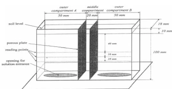
We used a bidimensional set up, by constructing two experimental boxes, 0.1 m high, 0.120 m wide and 0.018 m deep from acrylic (Figure 1). In these boxes a middle compartment was separated from the outer compartments by two porous plates, 0.0015 m thick. These plates allowed water and nutrients to move from one compartment to the other, but they acted as a barrier to any roots.
An opening in the bottom of each outer compartment was covered with a nylon tissue, to allow the entrance of water and dissolved nutrients into the soil. After saturation of the porous plates the three compartments of each box were filled to about 0.01 m from the top with soil material from the subsurface layer of a very clayey oxisol (720 g kg-1 clay; 110 g kg-1
silt; 170 g kg-1 sand) from the county of Piracicaba,
São Paulo State, Brazil. The boxes were then put into another container which was filled to a depth of about 0.03 m with a nutrient solution containing adequate concentrations of all essential plant nutrients. The outsides of the boxes were subsequently covered with foam to avoid excessive rises in temperature and the growth of algae. Five rice seeds were sown in the middle compartment of the boxes which were then put in a greenhouse. The first seedlings emerged about four days after planting. A few days after emergence
the soil surface was covered with a layer of about 0.01 m of very coarse sand to reduce subsequent water loss by evaporation. The nutrient solution was renewed weekly. At 16 days after emergence the smallest plants were removed, leaving only three plants per box. At 43 days after emergence the supply of the solution was stopped and the boxes were allowed to drain. The very next day, the openings in the bottom of the outer compartments were closed with tape and the subsequent soil water depletion was monitored using a γ-beam attenuation method as described below. By then the rice roots had filled and dried out the middle compartment and all water taken up came from the outer compartment through the porous plates which, therefore, could be considered as an extension of the root surface. In this bidimensional set up, equation 9 becomes
ψ
m xψ
m sr R x
x
TA
A
K
dx
t
,
=
,+
∫
1
(10)
where Ar (m2) is the total root area. In our set up
(Figure 1) A equals 3.6.10-4 m2 (0.02 x 0.018 m) and Ar equals 3.24.10-3 m2 (2 x 0.09 x 0.018 m).
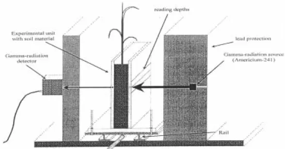
Monitoring soil water depletion - Soil water depletion was monitored using γ-beam equipment from the Center for Nuclear Energy in Agriculture (CENA) in Piracicaba, São Paulo State, Brazil. 241Am
with a γ-energy of 59.6 keV and an activity of 3.7.109 Bq was used as the γ source. Figure 1 shows
the configuration of the γ source experimental box -γ detector. The γ beam collimators had a diameter of 0.004 m and were enclosed in lead blocks. The collimating distance was 0.030 m on the side of the γ source and 0.020 m on the side of the detector. The maximum collimating divergence was 0.05 rad. The γ count time was 6 seconds.
Readings were made over a period of 12 days, until wilting of the plants. For each reading, the experimental boxes were put on a traveling rail so they could be repositioned precisely between the γ source and the detector (Figure 2). Readings were made at 3 depths (0.04, 0.05 and 0.06 m) along the whole extent of both outer compartments of each box, at intervals of 0.0014 m. This procedure resulted in about 36 reading points at each depth (Figure 1). As roots are confined to a very small volume, we may assume that there is no difference between the uptake pattern at the three depths, and data can be considered as replications giving a total of twelve replications (2 boxes x 3 depths x 2 sides).
According to the Lambert-Beer equation it follows that the volumetric soil water content θ (m3 m-3) is
given by
θ
=
µ ρ
ln
I
I
x
w w
0
(11)
where I0 (photons m-2 s-1) is the measured beam
intensity through the experimental box containing only oven-dry soil, I (photons m-2 s-1) is the measured
beam intensity during the experiment, µw (m2 kg-1) is
the mass-attenuation coefficient for water at a given γ-energy, ρw (kg m-3) is the density of water and x (m)
is the total soil thickness.
Values of I0 were determined at the end of the
experiment by oven-drying the experimental boxes with soil and then remeasuring the γ beam intensity at each reading point. The value of µw was determined
by measuring γ attenuation of pure water.
To determine the soil water retention curve and the soil bulk density, three cylinders were filled with the same soil as the experimental boxes and treated
in the same way (i.e., they were submitted to the same nutrient solution) so that the soil physical properties would be the same in the boxes and in the cylinders. The diameter of the cylinders was 0.05 m and they were composed of three sections, an upper and a lower section 0.045 m high and a middle section 0.010 m high. After finishing the γ attenuation experiment, the sections were separated. The upper section was discarded. The lower section was used to determine the soil bulk density. The middle section was used to determine the soil water retention curve by submitting it to suctions of 0.49, 0.98, 1.96, 3.92, 5.89, 7.85 and 9.81 kPa using a porous plate funnel and to pressures of 10, 18, 36, 90, 230, 595 and 1490 kPa using a pressure plate apparatus. The water retention data were fitted to the Van Genuchten (1980) equation:
(
)
[
]
θ θ
θ θ
α ψ
=
+
−
+
r s r m n m1
(12)where θr (m3 m-3) is the residual water content, θs
(m3 m-3) is the saturated water content and α (kPa-1), m and n are the empirical parameters of the equation. The soil’s hydraulic conductivity (K, m2 kPa-1 s-1)
as a function of soil water content was estimated using a method presented by Reichardt and Libardi (1974). Firstly, the hydraulic diffusivity (D, m2 s-1) was
estimated by the empirical function
D
=
−f e
− −
8 770 10
4 2 8 0870 1 0
.
.
. ( ) ( ) θ θθ θ (13)
with θ0, θ1 and f determined from a horizontal
infiltration experiment. θ0 (m3 m-3) is the antecedent
soil moisture content, θ1 (m3 m-3) is the soil moisture
content at the end of the experiment. The parameter
f (m s-0.5), known as sorptivity, is the slope of the line
that describes the advance of the wetting front as a function of the square root of time. To determine the value of f the soil was packed into an acrylic plastic cylinder having an inside diameter of 0.055 m and a length of 0.50 m. The soil was packed at the same bulk density as observed in the experimental boxes (1168 kg m-3). Water was applied to the inlet end of
the cylinder at an effective pressure of -0.3 kPa (measured from the center of the cylinder) through a fritted glass plate of medium coarse porosity. Once infiltration was begun the distance from the water source to the wetting front was recorded over a series of time intervals. The parameter f was later determined by linear regression of x versus t0.5.
Hydraulic conductivity is related to the hydraulic diffusivity by the equation
K
D
d
d
m=
θ
ψ
(14)Replacing dθ/dψm by the first derivate of equation 12 results in the following expression:
(
)
(
)
[
]
K
D
s rmn
n m n m n m=
−
+
− +θ θ
α ψ
α ψ
1
1
1
(15)Substitution of (13) and (15) in (10) results in:
(
)
( )
ψ
ψ
θ θ
α
ψ
αψ
θ θ θ θ
m x m s
s r n r m x n m x n m R x
TA
f
mn
A
e
dx
x t , , . , ,. .
.
.
=
+
−
+
− − −− − +∫
8 7710
1
4 28 087 0 1 1
1 0 (16)
The analytical solution of equation 16 is not possible, because of the appearance of the parameter ψm,x on both sides of the equation. Thus particular
solutions must be obtained by numerical methods. Knowing the extension of the depletion zone (Rt) and the values of parameters related to the soil (α, m, n, θr, θs, ψs, f, θ0, θ1), to the plant (A, Ar) and to the
atmosphere (T) a value of ψx can be calculated for
each x.
Transpiration rates were estimated from variation in observed soil water contents using the expression
(
)
T
V
AL t
t t tdL
L=
2
∫
+−
0
∆
θ
∆θ
(17)where
θ
(m3 m-3) is the mean soil water contentobserved at the three depths and in both compartments of the experimental boxes, V (m3) is
the total volume of the soil-filled part of the outer compartments (V = 1.62.10-4 m3), L (m) is the length
of the outer compartment (L = 0.05 m) and ∆t (s) is the time between two subsequent readings (∆t = 86,400 s or 172,800 s).
Knowing T, A, f, θs, θr, a, m, n, Ar, θ0 and q1, the
advance of the depletion zone, soil moisture content outside the depletion zone (θsoil, m3 m-3) and root
surface potential (ψroot, kPa) were determined by non-linear iterative fitting of equation 13 to the measurements of soil water content, using a distance increment of 0.0001 m. Observed and simulated soil water contents within the depletion zone were compared, calculating the coefficient of determination (r2) and the degree of agreement (M), with
(
)
(
)
r i i i n i i n 2 2 1 2 1 1 = − − − = =∑
∑
$ $ θ θθ θ (18)
M n i i i n = − =
∑
θ$ θθ
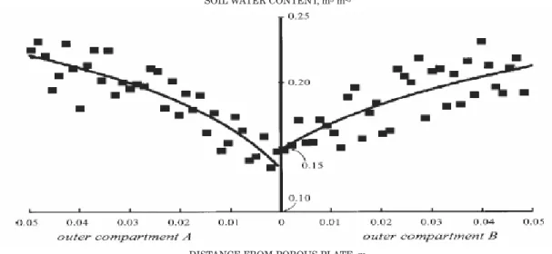
Now, observed soil water contents in the experimental boxes were compared to those expected by equation 16. As an example, figure 4 shows soil water contents measured at 0.04 m depth in both outer compartments of one of the two experimental boxes, 10 days after the water supply was stopped, together with the fitted line.
Calculations of the soil matric potential as a function of distance from the root surface as estimated by equation 16 are shown in figure 5. Mean values for
T, Rt, θsoil and ψroot and the statistics associated with
each fit are presented in table 1.
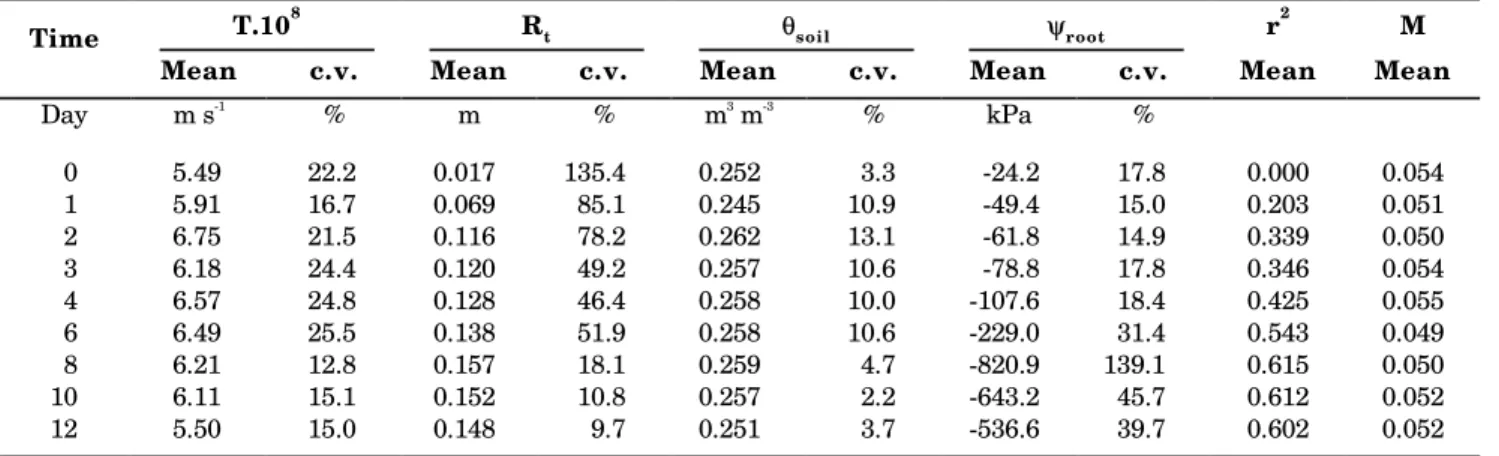
Transpiration rates, as calculated by equation 17, are fairly constant throughout the 12 days of the experiment. Some decline is observed at the end of the experiment, although the values do not become lower than those of the first days. This indicates that,
Table 1. Mean values of transpiration (T), advance of the drying front (Rt), soil water content outside the
depletion zone (θθθθθsoil,), root potential (ψψψψψroot) and r2 and M values, and coefficients of variation (c.v.), for
the 9 reading dates
Time T.10
8
Rt θsoi l ψroot r2 M
Mean c.v. Mean c.v. Mean c.v. Mean c.v. Mean Mean Day m s-1
% m % m3
m-3
% kPa %
0 5.49 22.2 0.017 135.4 0.252 3.3 -24.2 17.8 0.000 0.054
1 5.91 16.7 0.069 85.1 0.245 10.9 -49.4 15.0 0.203 0.051
2 6.75 21.5 0.116 78.2 0.262 13.1 -61.8 14.9 0.339 0.050
3 6.18 24.4 0.120 49.2 0.257 10.6 -78.8 17.8 0.346 0.054
4 6.57 24.8 0.128 46.4 0.258 10.0 -107.6 18.4 0.425 0.055
6 6.49 25.5 0.138 51.9 0.258 10.6 -229.0 31.4 0.543 0.049
8 6.21 12.8 0.157 18.1 0.259 4.7 -820.9 139.1 0.615 0.050
10 6.11 15.1 0.152 10.8 0.257 2.2 -643.2 45.7 0.612 0.052
12 5.50 15.0 0.148 9.7 0.251 3.7 -536.6 39.7 0.602 0.052
where n is the number of observations,
θ
iand θ$i are
the i-th observed and simulated soil water content, respectively, and
θ
is the mean observed soil water content.RESULTS AND DISCUSSION
Soil moisture values obtained for the different matric potentials fitted very well to equation 12. Figure 3 shows the soil water retention data, the fitted curve and the empirical parameters for the equation. The determination of f (equation 13) in the horizontal infiltration experiment resulted in a value of 0.000698 m s-0.5 with θ
0 = 0.0308 m3 m-3 and
θ1 = 0.4863 m3 m-3.
MATRIC POTENTIAL, -kPa
Figure 3. Soil water retention curve with experimental data and fitted line.
SOIL W
A
TER
CONTENT
,
m
3 m
Figure 4. Example of measured soil water contents (dots) and model estimates after fitting to equation 16 (line) for observations made 10 days after the water supply was stopped, at 0.04 m depth, in both sides of the experimental box.
DISTANCE FROM ROOT SURFACE, m
MA
TRIC PO
TENTIAL,
k
P
a
Figure 5. Matric potential as a function of distance from the root surface for the nine reading dates as estimated by equation 16 after fitting to the experimental data.
although root potentials become more and more negative and wilting symptoms were observed above ground, soil water extraction still continued at a rather high rate.
Table 1 shows that r2 values, as calculated by
equation 18, increase up to about 0.6 by the end of the experiment. Very low values were obtained during the first days of observations. However, good fitting during the whole period is evidenced by the low M values (equation 19), pointing out mean differences of about 5% between observed and estimated values, indicating that the low r2 values are a mere reflection
of the fact that the shape of the curve that describes matric potential as a function of the distance to the root surface behaved much like a straight horizontal line during the first days.
Root surface potential diminished until day 8 to a minimum value of approximately -820 kPa. The more negative ψroot values are associated to high coefficients of variation. This is explained by the fact that we measured θ and relatively small errors in θ result in
high differences in ψ, due to the shape of the θ-ψ curve (Figure 3). For example, from equation 12, we calculate that -820 kPa corresponds to θ = 0.140 m3 m-3, while
-1500 kPa, almost twice as negative, corresponds to the only slightly lower value of θ = 0.134 m3 m-3.
Within one percent of soil moisture content, soil matric potential values double.
Soil water contents diminished by an average value of 0.05 m3 m-3, within 12 days, resulting in a dθ/dt of
about -5.10-8 s-1. Application of the water conservation
equation shows a mean underestimation of flux densities within the extent of the outer compartments of 1.2.10-9 m s-1 (5.10-8 s-1 x 0.025 m) Transpiration
rates of about 6.10-8 m s-1 result, in our experimental
setup, in flux densities of about 8 . 10-9 m s-1.
Therefore, by neglecting soil water content variation within the outer compartments when estimating flux densities, we are in fact slightly overestimating root surface potentials.
Values of θsoil, soil water content outside the
depletion zone, should be expected not to vary during
SOIL WATER CONTENT, m3 m-3
the experiment, and they practically didn’t. Values are around 0.25 m3 m-3, corresponding to a matric
potential of approximately -23 kPa, within the range normally considered as “field capacity”, and close to the initial ψroot value. The extension of the depletion
zone, Rt, is associated to high coefficients of variation until day 6. During these days, soil water depletion had not yet much advanced, and the matric potential as a function of distance from the root surface was little different from a straight horizontal line (Figure 5). Therefore, small differences in observed values caused great differences between estimated Rt
values for the same day. It should be remembered that these values, as well as the θsoil values, are estimated
values, extrapolated by regression, and no observed values. As a matter of fact, they couldn’t possibly have been observed, as the dimensions of the experimental boxes were much smaller than the majority of the Rt
values. From the second day on, we estimated Rt
values of more than 0.10 m. This means that our model shows that a single plant root is able to extract water from a distance of more than 0.10 m in only 2 days. Although, initially in small quantities, we can see that, as depletion continues, considerable quantities of water are extracted from remote distance from the root. This indicates that, at least in soils with hydraulic conductivities comparable to those of our soil, root distribution may play a less important role in the efficiency of water uptake, as long as distances between neighboring roots do not exceed something in the order of 0.10 m. This conflicts with earlier conclusions of Gardner (1964) and of Tardieu et al. (1992), who found that spatial arrangement did influence water uptake efficiency, and reinforces the hypothesis that major resistance to soil water flux may occur in other parts of the soil-plant continuum, e.g. at the soil root interface (Faiz & Weatherley, 1982) or within the plant xylem (Taylor & Klepper (1975); Molz (1976); Blizzard & Boyer (1980).
CONCLUSIONS
Comparisons between model output and experimental results suggest the model here developed can describe the extraction of soil water by a plant root. Model simulations show that a single plant root is able to withdraw water from more than 0.1 m away within a few days. We therefore can assume that root distribution may be a less important factor for soil water extraction efficiency.
REFERENCES
BLIZZARD, W.E & BOYER, J.S. Comparative resistance of the soil and the plant to water transport. Plant Phys., Rockville, 66: 809-814, 1980.
CARBON, B.A. Diurnal water stress in plants grown on a course soil. Austr. J. Soil Res., Melbourne, 11:33-42, 1973.
COWAN, I.R. Transport of water in the soil-plant-atmosphere system. J. Appl. Ecol., Oxford, 2:221-239, 1965.
FAIZ, S.M.A. & WEATHERLEY, P.E. Root contraction in transpiring plants. New Phytol., Cambridge, 92:333-343, 1982.
GARDNER, W.R. Dynamic aspects of water availability to plants. Soil Sci., Baltimore, 89:63-67, 1960.
GARDNER, W.R. Relation of root distribution to water uptake and availability. Agron. J., Madison, 56:41-45, 1964.
GARDNER, W.R. & EHLIG, C.F. Some observations on the movement of water to plant roots. Agron. J., Madison, 54:453-456, 1962.
GARDNER, W.H.; CAMPBELL, G.S. & CALISSENDORFF, C. Systematic and random errors in dual gamma energy soil bulk density and water content measurements. Soil Sci. Soc. Am. Proc., Madison, 36:393-398, 1972.
HAINSWORTH, J.M. & AYLMORE, L.A.G. Water extraction by single plant roots. Soil Sci. Soc. Am. J., Madison, 50:841-848, 1986.
HILLEL, D.; BEEK, C.G.E.M. VAN & TALPAZ, H. A microscopic-scale model of soil water uptake and salt movement to plant roots. Soil Sci., Baltimore, 120:385-399, 1975.
HILLEL, D.; TALPAZ, H. & KEULEN, H VAN. A macroscopic model of water uptake by a nonuniform root system and of water and salt movement in the soil profile. Soil Sci., Baltimore, 121:242-255, 1976.
HULUGALLE, N.R. & WILLATT, S.T. The role of soil resistance in determining water uptake by plant root systems. Austr. J. Soil Res., Melbourne, 21:571-574, 1983.
MACKLON, A.E.S. & WEATHERLEY, P.E. Controlled environment studies of the nature and origins of water deficits in plants. New Phytol., Cambridge, 64:414-427, 1965.
MOLDRUP, P.; ROLSTON, D.E.; HANSEN, J.A. & YAMAGUCHI, T. A simple mechanistic model for soil resistance to plant water uptake. Soil Sci., Baltimore, 153:87-93, 1992.
MOLZ, F.J. Water transport in the soil-root system: transient analysis. Water Resour. Res., Washington, 12:805-808, 1976. MOLZ, F.J. & REMSON, I. Extraction term models of soil moisture
use by transpiring plants. Wat. Resour. Res., Washington, 6:1346-1356, 1970.
NIMAH, M.N. & HANKS, R.J. Model for estimating soil water, plant and atmospheric interrelations: I. Description and sensitivity. Soil Sci. Soc. Am. Proc., Madison, 37:522-527, 1973.
REICHARDT, K. & LIBARDI, P.L. A new equation to estimate soil-water diffusivity. Vienna, International Atomic Energy Agency, 45-51, 1974. (Isotope and Radiation Techniques in Soil Physics and Irrigation Studies 1973).
SLACK, D.C.; HAAN, C.T. & WELLS, L.G. Modeling soil water movement into plant roots. Trans. ASAE, St. Joseph, 20:919-927, 1977.
TARDIEU, F.; BRUCKLER, L. & LAFOLIE, F. Root clumping may affect the root water potential and the resistance to soil-root water transport. Plant Soil, The Hague, 140:291-301, 1992. TAYLOR, H.M. & KLEPPER, B. Water uptake by roots. Soil Sci.,
Baltimore, 120:57-67, 1975.
VAN GENUCHTEN, M.T. A closed-form equation for predicting the hydraulic conductivity of unsaturated soils. Soil Sci. Soc. Am. J., Madison, 44:892-897, 1980.
WHISLER, F.D.; KLUTE, A. & MILLINGTON, R.J. Analysis of steady-state evapotranspiration from a soil column. Soil Sci. Soc. Am. Proc., Madison, 32:167-174, 1968.