i
Index
1. INTRODUCTION ... 2
2. VOLATILITY MODELS ... 3
3. A BRIEF DESCRIPTION OF EXISTING TESTS ... 5
3.1 Diebold-Mariano (1995) ... 5
3.2 A modified Diebold-Mariano test... 10
3.3 A modified Morgan-Granger-Newbold test ... 13
3.4 Harvey, Leybourne, Newbold (1998) ... 18
3.5 Harvey and Newbold (2000) ... 24
3.6 Peter Hansen (2005) ... 30
4. STATISTICAL PROPERTIES OF RETURNS ... 39
5. ECONOMETRIC APPROACH ... 44
6. ESTIMATION RESULTS ... 48
In-sample results ... 48
Out-of sample results ... 55
7. CONCLUSION ... 62
8. THESIS LIMITATIONS AND FUTURE RESEARCH ... 63
2 1. INTRODUCTION
Forecasting can be described as an attempt to foresee the future by examining historical data. In simple terms, a forecast is an estimate for the future value of some variable. Therefore, forecasts may not be confused with guesses or intuition.
In corporate world, managers often predict future events based upon past experience and personal opinion. However, in these days of rapid change, where uncertainty is a reality/constant, forecasting is gaining weight in companies’ decisions, being a useful tool for managers. Forecasting is important not only for those who use it, but also for those who create them, since their reputation is directly related.
Given that forecasts play an important role in modern organizations, forecasting accuracy becomes extremely important. In spite the enormous amount of studies found in the literature, forecasting accuracy comparison does not emerge as an easy task, due to several limitations. When the first formal tests of forecasting accuracy came up, the conditions imposed to the loss function and the forecast errors where too restrictive. Specifically, and in accordance to Diebold (1995):
a) The loss function had to be quadratic
And the forecast errors needed to be:
b1) Zero mean b2) Gaussian
b3) Serially uncorrelated
b4) Contemporaneously uncorrelated
Because some of these conditions are difficult to obtain, recent efforts have been made to surpass them and new tests with the relaxation of some conditions were proposed. Indeed, over the last few years, several papers emerged, suggesting different statistical tests to deal with forecasting accuracy.
3 Thus, and due to the importance of this subject for empirical finance, the main purpose of this thesis is to make use of those tests to compare the forecasting capability of some alternative conditional heteroskedasticity models.
This thesis is organized as follows. Section 2 will present the volatility models to be used in our empirical application. Section 3 will review in a brief way the available literature related with forecasting accuracy tests. Data’s statistical properties can be seen in Section 4, while the econometric approach is given in Section 5. Estimation results will be discussed in Section 6 and the conclusions will be made in Section 7. Finally, Section 8 mentions some thesis limitations.
2. VOLATILITY MODELS
Due to the major importance played by risk in financial markets, and modeling and forecasting volatility In fact, modeling and forecasting volatility has become a true focus of attention over the last few years
As early noted by Mandelbrot (1963) and Fama (1965), financial time series vary systemically with time and tend to display periods of unusual large volatility, followed by periods of low volatility. With these findings, Mandelbrot and Fama pointed out the importance of volatility in financial markets. Despite their early findings, however, the efforts to model and forecast volatility only occurred over the last two decades and centered their attention in some stylized facts of asset returns.
Bollerslev et al (1994) pointed out eight empirical regularities of asset returns:
1. Asset returns tend to be leptokurtic;
2. Returns are not i.i.d. (independent and identically distributed) through time. This phenomenon is also known as volatility clustering;
3. Also known as Fisher-Black effect, the leverage effect states that volatility and asset returns are negatively correlated. In other words, price’s changes of the same magnitude but different signs will reflect differently in volatility. Specifically, volatility will increase more after a negative change in the asset’s price;
4 4. Information that accumulates when financial markets are closed is reflected in
prices after the markets reopen;
5. Forecastable releases of important information are associated with high ex ante volatility. For example, individual firms’ stock returns volatility is high around earnings announcements;
6. Volatility and serial correlation are inversely correlated;
7. As observed by Black (1976), a 1% market volatility change typically implies a 1% volatility change for each stock;
8. Measures of macroeconomic uncertainty help to explain changes in stock market volatility.
The first model that seemed to be able to capture some of these stylized facts was proposed by Engle (1982), who launched the first ARCH (autoregressive conditional heteroskedasticity) model. In ARCH (q), the conditional variance is a function of the past q squared innovations. Later, Bollerslev (1986) proposed a generalization of Engle’s model, known as GARCH (generalized autoregressive conditional heteroskedasticity), a more parsimonious model than ARCH, as empirical findings suggest. The GARCH (p,q) permits additional dependencies on p lags of the past conditional variance. GARCH (1,1) is the most popular structure for many financial time series.
Although ARCH and GARCH models proved to be able to capture the volatility clusters stylized fact of returns and partially describe the fat tails exhibited by financial data time series, two drawbacks can be pointed out. First, they discharge any influence of the innovations’ sign in the conditional variance. Instead, they assume that only the innovations’ magnitude is relevant, neglecting the leverage effect. The other ARCHER limitation has to do with the parameters non-negativity restrictions, meaning that they can assume any value, even a negative one.
These limitations led some authors to propose new models. Among them, the EGARCH and the GJR models that will be used in this study.
5 The EGARCH (Exponential GARCH) model (Nelson, 1991) was constructed in a way that a negative shock leads to a higher conditional variance in the subsequent period than a positive shock would. In other words, EGARCH was constructed to account for the leverage effect. For that reason, the conditional variance is specified in logarithmic form, so that the conditional variance depends on both the size and the sign of lagged residuals. That way, there is no need to impose estimation constraint in order to avoid negative variance.
The GJR model was proposed by Glosten et al. (1993) and is very similar to the Threshold GARCH (TGARCH) model (Zakoian, 1994). “GJR allows a quadratic response of volatility to news with different coefficient for good and bad news, but maintains the assertion that the minimum volatility will result when there is no news (Bolleslev et al, 1994: 2970).” In this model, the leverage effect is modeled with a dummy variable that assumes the value 1 to represent a negative shock and 0 otherwise
In the following section, we will present the accuracy tests that will be used to compare these models in our empirical study.
3. A BRIEF DESCRIPTION OF EXISTING TESTS
3.1 Diebold-Mariano (1995)
Consider two forecasts, and , of the time series . Let the associated forecast errors be and , respectively. We wish to assess the expected loss associated with each of the forecasts. Thus, let us consider
and as the loss functions.
The null hypothesis of Diebold-Mariano test states that there is no difference between two competing forecasts, in terms of their accuracy skill. Equivalently, the null hypothesis states that the population mean of the differential loss is zero ( , where is the loss differential).
6 In contrast with the previously developed tests, Diebold-Mariano (1995) test allows the loss function to be non-quadratic and asymmetric. Besides, errors can be non-Gaussion, non-zero mean, serially correlated and contemporaneously correlated.
Diebold-Mariano test statistic is the following:
, (1)
where is a consistent estimate of , the spectral density of the loss differential at frequency 0 and is the sample mean loss differential which, in large samples, is approximately normally distributed with mean µ and variance .
Diebold and Mariano evaluated the finite-sample size of several test statistics, under the null hypothesis. Besides S1, two finite-sample reference tests were included in this study: the sign test (S2) and the Wilcoxon’s signed-rank test (S3). The studentized versions of these two tests (S2a and S3a, respectively) were also studied.
, (2) where (3) (4)
(5)
7 Moreover, the F-test, as well as the MGN (Granger and Newbold, 1977) and MR (Meese and Rogoff, 1988) tests were also included in this analysis.
F-test
The F-test requires all previous referred assumptions to be valid. The null hypothesis of equal forecast accuracy corresponds to equal forecast error variances (by 1 and 2a). By the remaining assumptions, the ratio of simple variances has the usual F distribution under the null hypothesis. Distributed as , the test statistic is:
(6)
This test statistics has little practical use due to the conditions imposed to the forecast errors which, as referred before, are very difficult to obtain.
Morgan-Granger-Newbold (1977)
In order to solve the contemporaneous correlation problem, Granger and Newbold employed an orthogonalizing transformation due to Morgan (1939-1940), enabling the relaxation of assumption b4. Thus, the Morgan-Granger-Newbold (MGN) test allows forecast errors to be contemporaneously correlated and maintains all the previously referred assumptions. Under this assumptions, the null hypothesis of equal forecast accuracy is equivalent to zero correlation between x and z ( ), where
and
and
Distributed as Student’s t with T-1 degrees of freedom, MGN test statistic is the following:
8 (7)
Meese-Rogoff (1988)
Like the MGN test, the Meese-Rogoff (MR) test allows forecast errors to be contemporaneously correlated. In addition, forecast errors can also be serially correlated. Under the remaining assumptions (a, b1 and b2), MR test is asymptotically distributed as standard normal and the test statistic is the following:
(8)
where and is a consistent estimator of ∑.
It is interesting to note that MR can coincide asymptotically with MGN, when the null hypothesis and assumptions a, b1, b2 and b3 are satisfied.
In these tests’ evaluation, Diebold and Mariano presented results for different levels of contemporaneous correlation (ρ), serial correlation (θ) and sample size (T). Gaussian and non-Gaussian forecast errors are also distinguished. Results are shown in the appendix (Tables 26-31).
Let us first discuss the case of Gaussian forecast errors. Here are summarized the main conclusions:
F is correctly sized when there is no contemporaneous and serial correlation (i.e. ρ = θ = 0) but is missized when any of them is present. Serial correlation pushes empirical size above nominal size, while contemporaneous correlation pushes empirical size severely below nominal size. Clearly, contemporaneous correlation dominates serial correlation. Therefore, in presence of both, F is undersized. This outcome is particularly apparent for large ρ and θ.
9 As expected, the MGN test remains correctly sized as long as θ = 0. As we already mentioned, the MGN test allows forecast errors to be contemporaneously correlated. Serial correlation, however, pushes empirical size above nominal size.
The results obtained for the MR test offer no surprises. As already mentioned, the MR test is robust to both serial and contemporaneous correlation. Indeed, for large samples (T>64), that proved to be truth. Still, in small samples, the MR test showed to be oversized in the presence of serial correlation.
In large samples, the S1 test showed to be robust to both contemporaneous and serial correlation. In small samples, however, S1 is oversized, a behavior particularly similar to the one showed by the MR test, except that the empirical and nominal sizes of the S1 test converge a bit more slowly, when compared to the MR test.
Finally, both S2 and S3 tests attested to perform well, with nominal and empirical size in close agreement, independently of contemporaneous or serial correlation, as well as sample size. Moreover, this conclusion can be extended to S2a and S3a tests.
In relation to non-Gaussion forecast errors, the most evident result is the drastic missizing of the F, MGN and MR tests, evidence that is common to both small and large samples. S1, S2a and S3a, on the other hand, maintain approximately correct size, except for very small sample sizes (T<32). In those cases, S2 and S3 continue to perform well.
To summarize, Figure 1 illustrates, in a really perceptible manner, the behavior verified by the F, MGN, MR and S1 tests, for the non-Gaussion case with ρ = θ = 0,5.
10 Figure 1: Empirical size, Four Test Statistics; Fat-Tailed case; Theta = Rho = 0,5
3.2 A modified Diebold-Mariano test
As showed before, the original DM test (S1) performs relatively well for large samples (T>32) but, for small and moderate samples, the test can be quite seriously oversized. Besides, this problem becomes progressively more severe as the forecast horizon grows. So in 1997, Harvey, Leybourne and Newbold proposed some modifications to the original DM test, with the purpose to improve the test’s performance for smaller samples. The authors employed an approximately unbiased estimator of the variance of and proved that:
, (9)
11 Therefore, the modified DM test statistic becomes:
(10)
where S1 is the original statistic, n is the number of observations and h is the number of steps-ahead forecasts.
Besides the test statistic, the modified DM test differs from the original one in another way. While the latter uses the critical values of the standard normal distribution, the former uses the critical values of the Student’s t distribution with (n-1) degrees of freedom.
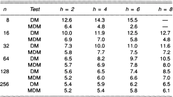
In order to conclude about the effects caused by these two modifications, the authors confronted the original Mariano test (DM) with the modified Diebold-Mariano test (MDM). The results appear in Table 1. Expected squared errors were taken as the criterion of forecast quality, so that .
12 Table 1: Percentage of rejections of the true null hypothesis of equal mean squared errors for the original and modified Diebold-Mariano test at nominal 10% level
13 As pointed out by Diebold and Mariano, their test has showed to be oversized for the case h=2. As we can see in Table 1, this problem is extended to longer horizons. Moreover, it becomes increasingly harsh as we move forward into the forecast horizon. The performance achieved by the modified test proved to be significantly better. Nevertheless, the high performance verified for the smallest samples can be seen as casual since that, for longer forecast horizons, the size appears to deteriorate with increasing n before improving again.
When compared to the original DM test, the empirical and nominal sizes of the MDM test demonstrated to be closer to each other, especially for the smallest samples. This phenomenon also verifies when the errors are autocorrelated and there is contemporaneous correlation.
The results obtained when using contemporaneous correlation or serial correlation coefficients of 0.5 and 0.9 were a lot similar to those presented in Table 1. Furthermore, the authors discovered that the empirical and nominal sizes tended to move closer with increasing θ.
The most important conclusion to take is that both improvements showed to improve DM test’s performance, although the modification made to the test statistic proved to be the more effective one.
3.3 A modified Morgan-Granger-Newbold test
As pointed out by Diebold and Mariano, in relation to the MGN test, for errors from a Student’s t with 6 degrees of freedom (t6) generating process, the serial correlation pushes the empirical size above the nominal size, meaning the test is over-sized. Besides, this problem gets deeper as the sample size increases.
14 Although Diebold and Mariano have identified this phenomenon, they weren’t able to find any explanation. Later, in 1997, Harvey, Leybourne and Newbold concluded that the size distortions verified for the MGN test had to do with the inconsistent estimation of one parameter (D), caused by the non-verification of the assumption , in which the usual regression test on is based.
, (11)
where
; ;
Under the conditions of theorem 5.3 of White (1984, p.109), that can be applied in this situation,
, (12)
where
; ;
Since , that implies and, consequently, . Given that does not hold, parameter D is inconsistently estimated. Therefore, in order to solve this problem, the authors employed a consistent estimator of D and proposed a modified MGN test, with the following test statistic:
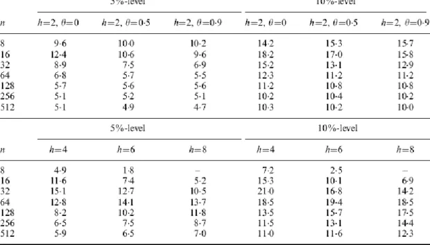
15 Although the null distributional result is no longer exact, the authors recommend the comparison this test statistic with critical values from the Student’s t distribution with (n-1) degrees of freedom. The comparison between the original and the modified MGN tests is presented in Table 2.
Table 2: Percentage of rejections of the true null hypothesis of equal one-step prediction mean squared errors for the original and modified Morgan-Granger-Newbold tests at nominal 10% level
Source: (Harvey et al., 1997:288)
Let us consider the original test in first place. Up to sampling error, the empirical size matches the nominal size. This result brings no surprises, since the null distribution is known in the normal case. However, for the t6 error-generating process, the test is seriously over-sized. Moreover, this problem gets deeper as the sample size increases. However, it seems that the excess size problem becomes less severe with increasing contemporaneous correlation between the forecast errors.
Concerning to the modified test, the conclusions are quite contradictory. As predicted by the theory, the modification created a test with the correct size for large samples. Nonetheless, performance in small samples, where the modified test is over-sized, is poor. In fact, in the smallest samples, the modified test is seriously over-sized when the error distribution is normal, and even worse than the original test for the t6 error-generating process. For that reason, the authors recommend the use of the modified MGN test only for moderately large samples.
16 Indeed, for the smallest sample sizes, the original MGN test proved to be more powerful than the modified one. Still, as the sample size increases, that advantage vanishes quickly.
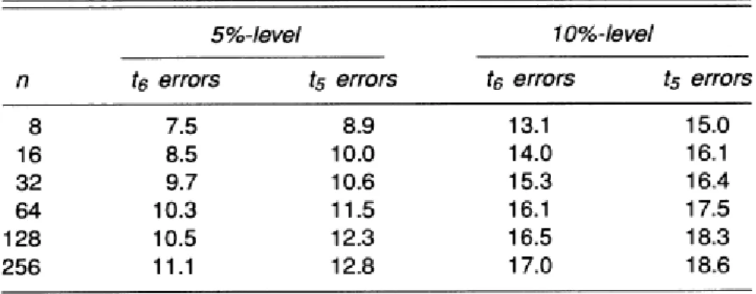
Since the test based on the modified statistic performed poorly in small samples, the authors considered also the possibility of a non-parametric approach. Specifically, the authors employed the Spearman’s rank correlation test because of their difficulty in handling non-normality. In Table 3, we can see a comparison between the MDM test, the rank correlation variant of the MGN test and the original version of the MGN test. The t6 generating process was considered for the former two tests.
Table 3: Percentage of rejections of the false null hypothesis of equal one-step prediction mean squared errors for the MDM, the rank correlation variant of MGN and the original MGN tests at 10% level
17 Through the analysis of Table 3, Harvey, Leybourne and Newbold came up with the following conclusions:
For the smallest sample sizes, the MGN test showed to be more powerful than the MDM test. Still, as the sample size increases, that advantage disappears.
For normal forecast errors, the performance verified by the rank correlation variant of the MGN test is pretty much identical with the performance of the MDM test, as well as the one demonstrated by the original MGN test for large samples. In small samples, however, most of the advantage of the MGN test is lost when ranks are employed.
In the case of heavy-tailed error distributions, the rank correlation test proved to be rather more powerful than the MDM test.
In conclusion, Harvey, Leybourne and Newbold recommend the use of the modified DM test, in part because of the lack of robustness of the MGN test in the presence of heavily-tailed distributions of the forecast errors. Besides, although the test based on rank correlations performs reasonably well, particularly for heavily-tailed error distributions, it is difficult to see how this test could be extended to deal with forecasts beyond one-step ahead.
18 3.4 Harvey, Leybourne, Newbold (1998)
When evaluating a forecast, it is often the case that several competing predictors are available. Harvey, Leybourne and Newbold investigated the issue of testing for forecast encompassing when there are two forecasts of the same quantity. The question to ask in these circumstances is whether any of the competing forecasts can add useful information not present in the superior forecast. If an inferior forecast contains no useful information, not present in the superior forecast, we say that the second forecast encompasses the first. In other words, “if a composite predictor formed as a weighted average of two individual forecasts is considered, then one forecast is said to encompass (or be conditionally efficient with respect to) the other if the inferior forecast’s optimal weight in the composite predictor is zero (Harvey and Newbold, 2000: 471)”.
Let be two competing forecasts of the quantity . One-step-ahead predictions were assumed (h=1). Let be the combined forecast, formed as a weighted average of the two individual forecasts,
, (14)
Then, if denote the errors of the individual forecasts and is the error of the combined forecast, we have:
(15)
In order to evaluate whether contains useful information not present in , Granger and Newbold (1973, 1986) proposed the estimation of regression (15) by ordinary least squares. The null hypothesis is .
When using a record of past forecast errors it is natural to test for forecast encompassing trough a simple least squares regression, which might be expected to perform well when forecast errors are generated by a bivariate normal distribution. However, in accordance to Harvey et al (1998), it was reasonable to suspect that forecast error distributions will often be heavily-tailed. In fact, they showed that, when forecast errors are normally distributed, we can stumble on far too many
19 rejections of a true null hypothesis of forecast encompassing. Consequently, they ran a simulation to evaluate the behavior of the standard regression-based test for forecast encompassing in finite samples. Results can be seen in Table 4.
Table 4: Empirical Sizes of Nominal 5%-level and 10%-level Regression-Based Tests for Forecast Encompassing
Source: (Harvey et al., 1998:256)
As can be noted, the oversizing problem becomes more severe as the number of sample observations increases, with very slow convergence to the asymptotic results found by the authors (0,122 and 0,171 for 5%-level; 0,182 and 0,230 for 10%-level).
Harvey et al. (1998) showed that the standard test for forecast encompassing can be incorrectly sized when the forecast errors are a temporally independent sequence but not normally distributed. “The non-normality problems associated with the standard regression-based test for multiple forecast encompassing can be shown to result from inconsistent estimation of the quantity Q, induced by conditional heteroskedasticity in the regression errors” (Harvey and Newbold, 2000: 473). Then, the most obvious modification in this situation is to employ the heteroskedasticity-robust estimator of White (1980), a procedure that can be extended to dependent error sequences.
Given this problem of lack of robustness to non-normality in the standard test,
, (16)
the authors proposed the following test that proved to be robust under these circumstances:
20
(17)
where is the sample mean of the sequence
Although is a consistent estimator for ,
convergence of the second term to zero is likely to be slow. This being the case, an alternative option is to replace the estimator by the estimator . Consequently, the authors proposed a new test statistic:
(18)
In both tests, the null hypothesis to be tested is of zero correlation between
and .
Harvey et al (1998) made a simulation experiment to evaluate finite sample sizes of R1 and R2 tests, along with the original DM test and the modified one proposed by Harvey et al (1997). For the standard DM test, normal critical values were used. For the other three tests, however, the authors used tn-1 critical values, given the results of Harvey et al (1997). Results appear in Table 5.
21 Table 5: Empirical Sizes of Nominal 5%-level and 10%-level Modified Regression-Based Tests and Diebold-Mariano-type Tests for Forecast Encompassing (h=1)
Source: (Harvey et al., 1998:257)
As predicted by theory, all four tests have approximately correct sizes in large samples. In small samples, however, the empirical and nominal sizes do not match, even when the forecast-error distribution is bivariate normal. A missizing can be noticed in R2 and MDM tests, whereas R1 and DM tests demonstrate to be oversized. In general, the MDM seems to perform better than its competitors and represents a distinct improvement on the standard regression-based test of the previous table when the generating process is bivariate Student’s t.
22 Given the general satisfactory size performance of the MDM test in the case h=1, the authors decided to investigate the test’s behavior for higher values of h (the steps-ahead forecast). The original DM test was also included in this simulation. Results are shown in Table 6.
Table 6: Empirical Sizes of Nominal 5%-level Diebold-Mariano-type Tests for Forecast Encompassing: Multistep-ahead Prediction (normal errors)
Source: (Harvey et al., 1998:258)
As we can see in Table 6, the empirical sizes of the MDM test are really close to the nominal sizes, except for long forecast horizons in small samples. Moreover, the MDM test is generally clearly preferable to the DM test in terms of size properties, suggesting that the Harvey et al (1997) modifications are well worth making.
The authors proceeded with further simulations, in order to verify if the power of the previous conclusions remain valid under a more general context. Specifically, for forecast horizons up to four, they also generated forecast errors from bivariate t5 and t6 distributions. The results found were relatively close from those for the case of normal errors. Therefore, we can confirm the robustness of the null distribution of the test statistics under heavy-tailed error distributions.
23 Finally, Harvey, Leybourne and Newbold made a power comparison of four tests for forecast encompassing. Those tests are the standard regression-based test R, the modified regression-based test R1, the MDM test and the Spearman’s rank correlation test (rs). Independent sequences of forecast errors (e1t,e2t) were generated from bivariate normal and bivariate t6 distributions and one-step–ahead forecasts were taken. We can see the estimated size-adjusted powers for the four tests in Table 7
.
Table 7: Estimated Size-Adjusted Powers of 5%-level Tests for Forecast Encompassing (h=1)
24 As expected, the most considerable differences among the tests occur at the smallest sample sizes, where R is clearly the most powerful of the four tests, for both normal and t6 errors. For samples inferior to 32, R1 is somewhat less powerful than R but more powerful than rs and manifestly more powerful than MDM. For sample sizes larger than 32, however, there is relatively little to choose among R, R1 and MDM. The poor power performance of MDM test in small samples - particularly for normally distributed errors - is quite regrettable, since its normal sizes are the more reliable ones. To make it worse, the nominal significance levels of R1 proved to be unreliable in these sample sizes (see Table 5) and the nominal significance levels of R cannot be trusted for any sample size (see Table 4). Therefore, the authors recommend the use of MDM over R and R1 tests. The same reason can be employed to choose MDM over R2, despite the identical size-adjusted power.
In relation to the correlation test, we can verify that it is slightly over performed by the other three tests, when we have a normal error distribution. When the error distribution is bivariate t6, however, the test performs relatively well, especially for large samples, where it beats all the other three tests. Hence, in the case in which the forecast errors are an independent sequence, the rank correlation test is certainly a viable alternative to MDM.
3.5 Harvey and Newbold (2000)
In 2000, Harvey and Newbold generalized the forecast encompassing approach to situations where there is more than one competing forecast to compare.
Let be K competing forecasts, taken to be unbiased or bias-corrected, of the actual quantity . Assume that the forecasts are made one-step-ahead, with non-autocorrelated errors. is the composite forecast.
, (19)
Equivalently,
25 where , and is the error of the combined forecast. The null hypothesis that encompasses its competitors is
(21)
The regression-based test for multiple forecast encompassing is an F-test of the joint significance of the parameters in equation (20).
It is convenient to note that regression (20) can be written as
, (21)
where
,
,
As this is a generalization of the two-forecast regression-based test studied by Harvey et al (1998), we expect to deal with the same problems, specifically, the lack of robustness to non-normality in the standard test, caused by conditional heteroskedasticity in the regression errors. Then, having this problem in mind, Harvey and Newbold presented three modified tests that proved to be robust to conditional heteroskedasticity in the regression errors. These tests also allow for forecast error autocorrelation, permitting comparison of forecasts made at horizons greater than one.
Modified regression-based tests
For the first two tests (F1 and F2), the authors followed the approach of the two-forecast case applied by Harvey et al (1998). Specifically, they employed the heteroskedasticity-robust estimator of White (1980), as well as a robust estimator which is consistent under the null, but not the alternative hypothesis.
26 In addition, they followed the proposition of Diebold and Mariano (1995) and Harvey et al (1998) that, for h-steps-ahead forecasts, a rectangular kernel with bandwidth (h-1) should be adopted to account for forecast error autocorrelation. The multivariate test statistics proposed by the authors is the following:
(22)
where , and have (i,j) elements
with and . Harvey and Newbold compare with the critical values from distribution.
Modified Diebold-Mariano test
Proposed by Harvey et al (1997), this test can be seen as an extension of the MDM test, being this the reason why it was named as the modified Diebold-Mariano-type test (MS*).
As showed before, in 1997, Harvey, Leybourne and Newbold proposed some modifications to the Diebold-Mariano test (1995), modifications that proved to be worth making. Later, in 1998, these authors found that the MDM test could be used to test for forecast encompassing, for the two competing forecasts case. Then, Harvey and Newbold (2000) generalized the test for multiple forecast encompassing. The new test statistic takes the form of Hotelling’s (1931) generalized T2
27 (23)
where
,
and is the sample covariance matrix. Although the finite sample result is not exact, Harvey and Newbold maintained the use of critical values.
Harvey and Newbold ran a simulation study to evaluate the finite sample behavior of the multiple forecast encompassing tests. Their results are displayed in Table 8. Forecast errors were generated from the multivariate normal distribution and the multivariate Student’s t-distribution with five and six degrees of freedom. Empirical sizes were calculated for nominal 5%-level and 10%-level tests. K=3 was used, meaning that they were testing whether one forecast encompasses two rival predictors.
Table 8: Empirical Sizes of Nominal 5%-level and 10%-level tests for K=3, h=1
28 As expected in theoretical grounds, for non-normal forecast errors, the F-test is incorrectly sized. Although it is common to both small and large samples, this over-sizing problem is more severe in the largest samples.
Relating to the other three tests, we can see that they have approximately correct size for the largest samples. For small and moderate samples however, we observe a drastic size distortion of the two modified regression-based tests. Specifically, the F1 test is over-sized and the F2 test is under-sized. In its turn, the MS* test has shown to be robust, although some under-sizing can be noticed in the smallest samples. These evidences are valid to both normal and non-normal errors.
Given the general satisfactory performance of the MS* test for one-step-ahead prediction, the authors investigated the test’s size properties when using forecasts made at horizons greater than one. For h=2, forecast errors were generated from MA(1) processes , while for larger h these errors were generated as white noise. As we can see in Table 9, the results are not as reliable as for one step-ahead prediction. Specifically, we can note some over-sizing for small samples and larger horizons.
Table 9: Empirical sizes of nominal 5%-level and 10%-level MS* tests for K=3 (normal errors)
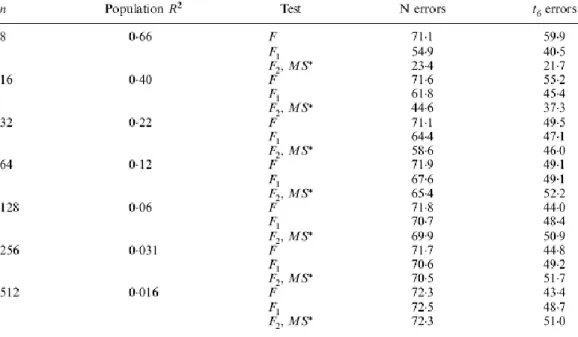
29 Now, we will see the estimated size-adjusted powers of each one of the tests for K=3, which are displayed in Table 10. The authors considered one-step-ahead forecasts with errors drawn from the multivariate normal and Student’s t6-distributions. Since MS* is a monotonic function of F2, these two tests have identical size-adjusted powers (see Harvey and Newbold, 2000).
Table 10: Estimated Size-adjusted Powers of 5%-level tests for K=3, h=1
Source: (Harvey and Newbold, 2000:479)
Through the analysis of Table 10 we can observe that, for large samples, the size-adjusted powers of the four tests are pretty much identical. For small and moderate samples however, the F-test displays the greater size-adjusted power. Given its superior power properties, the authors feel disappointed with the fact that the F-test is not robust to non-normality. Right after the F-test, we have the F1-test, followed by the MS* test and the F2-test. As we can see, the differences between the tests get smaller as the sample size increase. Also, they are more evident for normal errors than t6 errors. Finally, with no surprises, the tests exhibit higher power for normal errors.
After analyzing all the results, the authors recommended the use of the MS* test for moderately large samples, due to its good size and reasonable power properties. Still, they warn about this test limitations, when dealing with small samples: under-sizing for one-step-ahead forecasts, over-under-sizing for multi-step-ahead evaluation and low power.
30 3.6 Peter Hansen (2005)
In 2005, Hansen proposed a test for Superior Predictive Ability (SPA). When testing for SPA, the question of interest is whether any alternative forecast is better than the benchmark forecast. Testing for SPA is useful for a forecaster who wants to explore whether a better forecasting model is available, compared to the model currently being used to make predictions.
In contrast with the Equal Predictive Ability (EPA) tests, SPA tests were developed to compare more than two competing forecasts. “The distinction is important because the former leads to a simple null hypothesis, whereas the latter leads to a composite hypothesis (Hansen, 2005: 366).”
One of the main complications in composite hypotheses testing is that (asymptotic) distributions typically depend on nuisance parameters. The usual way to handle this problem is to use the least favorable configuration (LFC), which is sometimes referred to as “the point least favorable to the alternative”. However, Hansen (2003) proposed a different approach that leads to more powerful tests of composite hypothesis.
Before Hansen, White (2000) proposed a test for Superior Predictive Ability, known as the Reality Check (RC) for data snooping. Also known as data mining, data snooping “occurs when a given set of data is used more than once for purposes of inference or model selection. When such data reuse occurs, there is always the possibility that any satisfactory results obtained may simply be due to chance rather than to any merit inherent in the method yielding the results (White, 2000: 1115)” This is an almost inevitable difficulty when analyzing time-series data, since that there is only one record of information about a given variable of interest.
The test introduced by White provides simple and straightforward procedures for testing the null hypothesis: the best model encountered in a specification search has no predictive superiority over a given benchmark model.
When compared to the RC test, the Hansen test proved to be more powerful and less sensitive to the inclusion of poor and irrelevant alternatives. Hansen test differs from the RC test in two ways. First, a studentized test statistic is employed:
31 (24)
where is some consistent estimator of and .
denotes the performance of model k relative to benchmark at time t.
Second, a null distribution based on is invoked, where is a carefully chosen estimator for µ that conforms with the null hypothesis. Specifically, Hansen suggested the estimator:
(25)
where denotes the indicator function.
Consider the vector of relative performances, . Assuming that , the null hypothesis that the benchmark is not inferior to any of the alternatives is:
The advantages of the studentized test statistic and the sample dependent null distribution is that they don’t rely on stationarity, and are therefore expected to be useful in a more general context. Now, let us discuss each one of these modifications individually.
As shown by Hansen, studentizing the individual statistics will allow a comparison between objects measured in the same “units of standard deviation”. Not doing so, will result in a pointless comparison between objects measured in different units. There is one exception where the studentization may reduce the power that occurs when the best performing model has the largest variance. Since poor performing models also tend to have the most erratic performances, the author considered this case to be of little empirical relevance.
32 The second modification made by Hansen had to do with the possible erosion of RC’ power when poor alternatives are included in the analysis. In other words, the p-value associated to the RC test can be increased in an artificial way by adding poor forecasts to the set of alternative forecasts. Naturally, we want to avoid that. Given that the poor alternatives are irrelevant for the asymptotic distribution, a proper test should reduce the influence of these models, while preserving the influence of the models with . Having this problem in mind, Hansen constructed his test in a way that incorporates all models, while it reduces the influence of alternatives that the data suggest are poor.
Since the test statistics have asymptotic distributions that depend on µ and Ω, these are nuisance parameters. The traditional way to proceed in this case is to replace a consistent estimator for Ω and employ LFC over the values of µ that satisfy the null hypothesis. However, Peter Hansen showed that this approach leads to some rather unfortunate properties when testing for SPA. Therefore, he proposed an alternative way to handle the nuisance dependence of µ, where a data dependent choice for µ is used, rather than µ=0 as dictated by the LFC.
The estimator chosen by Hansen ( ) was motivated by the law of the iterated logarithm. According to this law:
, (26)
and
, (27)
This way, meet the necessary asymptotic requirements defined by Hansen. Estimator proved to account for the fact that poor alternatives should be discarded asymptotically but not in finite samples.
33 While separates correctly the good alternatives from the poor ones, there are other threshold rates that also produce valid tests. Because different threshold rates will lead to different p-values in finite samples, it is convenient to determine an upper and lower bound ( and , respectively).
(28)
(29)
where k=1,…,m.
In order to obtain the p-values of the three tests for SPA, Hansen followed a bootstrap implementation based on the stationary bootstrap of Politis and Romano (1994). Consequently, we will have six different tests to be estimated, a result of two test statistics (RC and SPA) and three null distributions (one for each estimator,
and ). Hansen studied the size and power properties of these six tests. The rejection frequencies of these tests at levels 5% and 10% can be seen in Tables 11, 12 and 13. Numbers in italic are used when the null hypothesis is true (Λ1 = 0). Numbers in standard font represent powers for the various local alternatives (Λ1 < 0).
34 Table 11: Rejection Frequencies under the Null and Alternative (m=100 and n=200)
35 Table 12: Rejection Frequencies under the Null and Alternative (m=100 and n=1000)
36 Table 11 contains the result for the case where m=100 and n=200. In the situation where all 100 inequalities are binding (Λ0 = Λ1 = 0), we see that the rejection probabilities are close to the nominal levels for all the tests. Trough the analysis of Table 11, it is possible to note that the SPAc-test has an over-rejection by 1%. However, this doesn’t seem to be problematic, since this over-rejection disappears when the sample size is increased to n=1000, as we can see Table 12. It is interesting to see that the liberal null distribution does not lead to a large over-rejection, which might be explained by a positive correlation across alternatives and a consequent positive correlation between the test statistic and . That way, the critical value will tend to be excessively small when the test statistic is small. Then, this correlation will reduce the over-rejection of the -based tests, suggesting that Hansen test can be improved. For that, it would be necessary to find a way to incorporate information about the off-diagonal elements of Ω.
Panel A corresponds to the case where µ=0, and is therefore the best possible situation for LFC-based tests. So this is the only situation where the LFC-based tests apply the correct asymptotic distribution. For that reason, it was expectable that the tests that are based on do well, which indeed happened. Fortunately, SPAc also performs well in this case. Turning to the configurations where Λ0 > 0, it is possible to notice the advantages of using the sample dependent null distribution. For example, in Panel E of Table 11, when (Λ0,Λ1) = (10,-3), while the RC almost never rejects the null hypothesis, SPAc-test has a power of approximately 84%.
Concerning to Table 13, we only notice a slight over-rejection when all inequalities are binding, (Λ0 = Λ1 = 0). The power properties are quite good, despite the fact that 1000 alternative are being compared to the benchmark.
37 Table 13: Rejection Frequencies under the Null and Alternative (m=1000 and n=200)
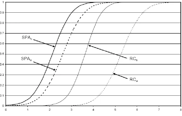
38 The power curves for the tests that employ and are shown in Figure 2, for the case where m=100, n=200 and Λ0=20. The power curves are based on tests that aim at a 5% significance level, and their rejection frequencies are plotted against a range of local alternatives. For the power curves in Figure 2, we conclude that the RC test is dominated by the three other tests. There is a significant increase in power when using the consistent distribution. Moreover, a quite similar improvement is achieved when we use the standardized test statistic, . In fact, according to Hansen’s calculations, to regain the power that is lost by using LFC instead of the sample dependent null distribution, it would be necessary a sample size 1.49 times larger, meaning that we are tossing 33% of the data when using the LFC. Besides, when we drop the studentization, a 65% of the data is being discarded. Dropping both modifications is equivalent to tossing away 84% of the data.
Figure 2: Local power curves of the four tests, SPAc, SPAu, RCc and RCu, for the simulation experiment where m=100, Λ0=20 and ranges from 0 to 8 (the x-axis). The power curves quantify the power improvements from the two modifications of the Reality Check.
39 4. STATISTICAL PROPERTIES OF RETURNS
Our data base is formed by the daily closing prices of the CAC40, FTSE100, NIKKEI 225 and S&P500 indexes from January 1, 1995 through December 31, 2009.1
In order to obtain the daily stock returns (rt), we followed the conventional procedure:
, (29)
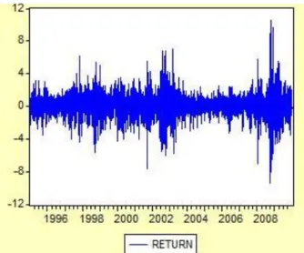
where Pt is the daily closing price of period t and Pt-1 is the daily closing price of period t-1. Figures 3, 4, 5 and 6 show us the behavior of our four indexes over time.
Figure 3: CAC40 returns
40 Figure 4: FTSE100 returns
41 Figure 6: S&P500 returns
It is evident that the ending of 2008 represent the most volatile period over the last 15 years, which is as a result of the sub-prime crisis that affected the whole world. Although it started in the USA, this crisis quickly spread all around the globe, as it can be confirmed by our four geographically scattered indexes (two from Europe, one from Asia and another one from Northern America). We can also identify another high volatility periods as for example: the October 1997 Asia mini-crash, the 1998 Russian financial crisis, the March 2000 dot-com bubble crash or the post-9/11 incident in 2001.
Table 14 provides a general overview of the data used.
Table 14: Statistical properties of returns
CAC40 FTSE100 NIKKEI225 S&P500
Observations 3803 3788 3686 3777 Mean 0,0193 0,015 -0,0169 0,0235 Median 0,0466 0,0504 0,0018 0,0683 Maximum 10,5946 9,3842 13,2346 10,9572 Minimum -9,4715 -9,2646 -12,111 -9,4695 Standard Deviation 1,483 1,2313 1,5822 1,2823 Skewness -0,0278 -0,1359 -0,1912 -0,2001 Kurtosis 7,6934 9,175 8,3519 11,1562 Jarque-Bera 3491,055 [0,0000] 6029,919 [0,0000] 4421,575 [0,0000] 10494,45 [0,0000]
42 As we can see, excepting NIKKEI225, the mean returns all are positive. NIKKEI225 also seems to be the most volatile index, since it has the lower and the high value, as well as the higher standard deviation. Without surprises, the Jarque-Bera test (Jarque and Bera, 1987) rejects the normality assumption for each of the series.
The Ljung-Box statistics on the returns, computed at a tenth-order lag, are shown in Figures 7, 8, 9 and 10.
Figure 7: Ljung-Box test for the CAC40 returns
43 Figure 9: Ljung-Box test for the NIKKEI225 returns
Figure 10: Ljung-Box test for the S&P500 returns
For the CAC40 index, the Ljung-Box test tells us that period t and period t-1 are not correlated, since we do not reject the null hypothesis at a 5% significance level. Still, we reject all the other null hypothesis, meaning that all the other autocorrelation coefficients are statistically significant at a 5% significance level.
44 Concerning the FTSE100 and the S&P500 indexes, it is possible to conclude that the returns are temporally correlated, since we reject (at a 5% level) the null hypothesis that the autocorrelation coefficients are equal to zero. Then, we can say that these series were not generated through a white noise process.
In its turn, for the NIKKEI225 index we can say that period t is correlated with period t-7, t-8 and t-9, if we assume a 10% significance level. For the remaining periods, we reject the null at a 5% level. Therefore, we conclude that every autocorrelation coefficient is statistically significant. That way, The NIKKEI225 returns were not generated through a white noise process.
Since we identified relevant autocorrelation in every index, we will consider an order five autoregressive model to remove the linear dependency in the series.
5. ECONOMETRIC APPROACH
The empirical distribution of a financial asset can be described as the sum of a predictable part with an unpredictable part:
, (30)
where is the relevant information set until, and including, t-1.
Based on our previous findings, we computed the conditional mean equation, , as a fifth-order autoregressive process, AR(5), in order to remove the observed linear dependency in the returns:
, (31)
where and the standardized innovations ( are assumed to be i.i.d. with Student’s t distribution.
Figures 11, 12, 13 and 14 show us the Ljung-Box test applied to the residuals after fitting the AR(5) to the series.
45 Figure 11: Ljung-Box test for the CAC40 residuals
46 Figure 13: Ljung-Box test for the NIKKEI225 residuals
Figure 14: Ljung-Box test for the S&P500 residuals
As we can see, the AR(5) successfully removed the linear dependency in CAC40, NIKKEI225 and S&P500 series up to the tenth-lag. For the FTSE100, however, the linear dependency was removed to the seventh-lag only, indicating that we could have used an autoregressive process of superior order than five. Still, the results obtained with the AR(5) are quite satisfactory and allow us to consider that the resides are now white noise.
47 For the conditional variance of , we have considered our three conditional heteroskedasticity models, GARCH, EGARCH and GJR.
As stated by Bollerslev et al. (1992) as well as Hansen and Lunde (2005), when modeling financial assets returns volatility, the (1,1) specification in ARCH (p,q) models is rather satisfactory. For that reason, we will use p=1 and q=1.
(32)
(33)
(34)
where are unknown parameters, if and if . All models were estimated through maximum likelihood (MLE).
Since volatility itself is not directly observable, establishing the effectiveness of the volatility forecast involves the use of a “volatility proxy” that may constitute an imperfect estimate of the true volatility, as mentioned by Andersen and Bollerslev (1998), for example. Following the conventional approach, squared returns are used as a proxy for the latent volatility process. According to Patton (2006) the squared return on an asset over the period t (assuming a zero mean return) is a conditionally unbiased estimator of the true unobserved conditional variance of the asset over the period t.
Our original sample was divided in two parts: the in-sample (January 3, 1995 to December 31, 2004) and the out-of-sample (January 3, 2005 to December 31, 2009). That way, the parameters for the conditional variance equation are estimated for the first ten years. The remaining five years were considered as the forecast period.
In the following section, we will present and discuss both in-sample and out-of-sample results.
48
6. ESTIMATION RESULTS2
In-sample results
Figures 15 to 26 report the in-sample results for CAC40, FTSE100, NIKKEI225 and S&P500. In order to compare these results, we will make use of three likelihood based goodness-of-fit criteria. Those criteria are the maximum log-likelihood, the Akaike Information Criteria (Akaike, 1978) and the Schwarz Bayesian Criteria (Scharwz, 1978). The first one is obtained from the maximum likelihood estimation and the bigger it is, the better it is. On the contrary, we want Akaike Information Criteria (AIC) and Schwarz Bayesian Criteria (SBC) to be as lower as possible.
Figure 15: Log-likelihood for GARCH (CAC40)
49 Figure 16: Log-likelihood for GJR (CAC40)
50 Figure 18: Log-likelihood for GARCH (FTSE100)
51 Figure 20: Log-likelihood for EGARCH (FTSE100)
52 Figure 22: Log-likelihood for GJR (NIKKEI225)
53 According to Tables 15-23, EGARCH is the best model to sculpt the conditional variance of CAC40, FTSE100 and NIKKEI225 returns. GJR comes in second place, leaving GARCH as the worst model. As expected, both asymmetric models (EGARCH and GJR) beat GARCH in terms of goodness-of-fit measures, proving that they successfully capture the leverage effect.
For the S&P500, however, the results are quite surprisingly, given that EGARCH is beaten by GARCH. Besides, GJR appears to be the most accurate predictor of S&P500 return’s volatility.
54 Figure 25: Log-likelihood for GJR (NIKKEI225)
55 Out-of sample results
In the out-of-sample analysis, we will use the tests presented in Section II to identify the best conditional heteroskedasticity model (GARCH, GJR or EGARCH). Specifically, we will use the Diebold-Mariano (1995), the modified Diebold-Mariano (1997), the modified Morgan-Granger-Newbold (1997), the Harvey-Leybourne-Newbold (1998), the Harvey-Harvey-Leybourne-Newbold (2000) and the Hansen (2005) tests.
It is important to note that these tests are measured in terms of their forecasting errors. Therefore, in order to choose the best model, we will choose the lowest test value, as we want to minimize forecasting errors.
According to the original Diebold-Mariano test (Tables 15 and 16), the conclusions are rather mixed.
Table 15: Diebold-Mariano test (MSE loss functions)
MSE
GJR-EGARCH GJR-GARCH EGARCH-GARCH
CAC40 -0,6331 [0,5266] -2,2020 [0,0267] -1,5028 [0,1329] FTSE100 -0,6058 [0,5447] -2,2895 [0,0221] -0,4768 [0,6335] NIKKEI225 -0,8069 [0,4197] -1,5563 [0,1196] -1,5865 [0,1126] SP500 -2,0376 [0,0416] -1,7054 [0,0881] 1,6137 [0,1066] Table 16: Diebold-Mariano test (MAE loss functions)
MAE
GJR-EGARCH GJR-GARCH EGARCH-GARCH
CAC40 2,2929 [0,0219] -3,0082 [0,0026] -3,7035 [0,0002] FTSE100 3,3451 [0,0008] -4,9535 [0,0000] -4,7296 [0,0000] NIKKEI225 2,5920 [0,0095] -0,3429 [0,7317] -3,9617 [0,0001] SP500 2,8888 [0,0039] -4,0828 [0,0000] -3,6106 [0,0003]
56 In terms of Mean Squared Errors (MSE) loss function, we point out two notes. First, GJR appears to beat GARCH, as we reject the null hypothesis that there is no difference in the accuracy of two competing forecasts and the test value is negative. Still, this is only true for CAC40 and FTSE100 (at 5% significance level) and SP500 (at 10% significance level). For NIKKEI225 the difference in the predictive accuracy is not statistically significant.
Second, GJR only beats EGARCH for the SP500 stock index. Thus, GJR seems to be the most appropriate volatility forecasting model, although this conclusion cannot be generalized to all the stock indexes under analysis. Also important is the fact that, in spite of the loss function being always lower for EGARCH (when compared to the symmetric GARCH), the differences are not statistically significant.
In terms of Absolute Squared Errors (MAE) loss function, the conclusions are somewhat clearer. As we can see in Table 16, with one exception, the null is always rejected, indicating accuracy differences among the competing models. The results point out to EGARCH as the best model to predict volatility, followed by GJR and lately, GARCH.
Without surprises, the values obtained for the modified Diebold-Mariano test (Tables 17 and 18) are practically the same of those we’ve found for the original test. Thus, the conclusions are exactly the same.
Table 17: Modified Diebold-Mariano test (MSE loss functions)
MSE
GJR-EGARCH GJR-GARCH EGARCH-GARCH
CAC40 -0,6329 [0,5268] -2,2011 [0,0277] -1,5022 [0,1330] FTSE100 -0,6055 [0,5448] -2,2886 [0,0221] -0,4766 [0,6336] NIKKEI225 -0,8066 [0,4199] -1,5556 [0,1198] -1,5859 [0,1128] SP500 -2,0368 [0,0417] -1,7047 [0,0883] 1,6130 [0,1067]
57 Table 18: Modified Diebold-Mariano test (MAE loss functions)
MAE
GJR-EGARCH GJR-GARCH EGARCH-GARCH
CAC40 2,2929 [0,0219] -3,0082 [0,0026] -3,7035 [0,0002] FTSE100 3,3451 [0,0008] -4,9535 [0,0000] -4,7296 [0,0000] NIKKEI225 2,5920 [0,0095] -0,3429 [0,7317] -3,9617 [0,0001] SP500 2,8888 [0,0039] -4,0828 [0,0000] -3,6106 [0,0003]
The values’ resemblance can be easily understood. Looking at equation (10) we conclude that the difference between these two tests depends on the number of h-step-ahead forecasts assumed. Since we use h=1, we can rewrite equation (10):
(35)
Given that, then,
As in the original and modified Diebold-Mariano tests, the null hypothesis of the modified MGN test also states that there is no difference in the accuracy of two competing forecasts.
Table 19: Modified MGN test
GARCH-EGARCH GARCH-GJR EGARCH-GJR
CAC40 0,0117 [0,9906] 0,0006 [0,9995] 0,0022 [0,9982] FTSE100 0,0018 [0,9986] 0,0000 [1,0000] 0,0030 [0,9976] NIKKEI225 0,0061 [0,9951] 0,1072 [0,9146] 0,0033 [0,9974] SP500 -0,0008 [0,9993] 0,0000 [1,0000] 0,0002 [0,9999]
58 Table 19 allow us to observe that, regardless the index, the null is never rejected. Then, we can conclude that GJR, GARCH and EGARCH are equally accurate, in terms of volatility prediction.
Harvey et al. (1998) proposed two tests to compare predictive ability of competing models. Let us discuss the results of those two tests (R1 and R2) individually.
Table 20: R1 test
R1
GARCH-EGARCH GARCH-GJR EGARCH-GJR EGARCH-GARCH GJR-GARCH GJR-EGARCH
CAC40 0,2689 [0,7880] 0,3234 [0,7464] 0,1201 [0,9044] -0,0401 [0,9680] -0,2493 [0,8031] -0,0133 [0,9894] FTSE100 0,1611 [0,8720] 0,0313 [0,9750] 0,1626 [0,8708] 0,0615 [0,9510] -0,0228 [0,9818] 0,0275 [0,9781] NIKKEI225 17,8633 [0,0000] 4,4203 [0,0000] 0,3680 [0,7129] -5,6295 [0,0000] -2,8792 [0,0040] -0,0120 [0,9904] SP500 0,0509 [0,9594] 0,7682 [0,4424] 0,4368 [0,6622] 0,5020 [0,6157] -0,4170 [0,6767] -0,0476 [0,9620] Table 21: R2 test R2
GARCH-EGARCH GARCH-GJR EGARCH-GJR EGARCH-GARCH GJR-GARCH GJR-EGARCH
CAC40 0,2119 [0,8322] 0,2444 [0,8069] 0,1365 [0,8914] -0,0386 [0,9692] -0,1996 [0,8418] 0,0132 [0,9895] FTSE100 0,1387 [0,8897] 0,0304 [0,9758] 0,1941 [0,8461] 0,0655 [0,9477] -0,0223 [0,9822] 0,0267 [0,9787] NIKKEI225 0,9470 [0,3436] 1,2924 [0,1962] 0,5823 [0,5604] -0,8492 [0,3958] -1,5321 [0,1255] -0,0121 [0,9903] SP500 0,0484 [0,9614] 0,4345 [0,6640] 0,7757 [0,4379] 1,0080 [0,3135] -0,2943 [0,7685] -0,0500 [0,9601]
A quick view over Tables 20 and 21 show a quite few contradictory results. Let us use the comparison of GARCH and EGARCH to illustrate that. Concerning to F1 test for the FTSE100 index, the value of the first row tell us that EGARCH encompasses GARCH, due to the positive and statistically significant test value. Logically, if EGARCH encompasses GARCH, then GARCH cannot encompass EGARCH. However, that’s the exact conclusion to be taken of the fourth row, where we have a positive and statistically significant value. Instead, we should have a negative value. Having this in mind, let us proceed to a more detailed analysis of the results.
59 Regarding R1, the conclusions are quite contradictory. For the CAC40 index, the positive and statistically significant values obtained in the three first rows indicate GJR as the best model, since it encompasses both GARCH and EGARCH. Also, EGARCH encompasses GARCH. The negative and statistically significant values obtained in the last three rows confirm this idea. For the other three indexes, the conclusions are not that clear. Specifically, for the FTSE100 index, we can only conclude that GJR encompasses GARCH, while for the S&P500 index, GJR seems to beat both GARCH and EGARCH. For the NIKKEI225 index, the most apparent result is GJR encompassing EGARCH.
Regarding R2 test, the most obvious outcome is the statistically significance of every single test value, indicating noteworthy differences among our three models. For the CAC40 index, the only conclusion to take is the fact that GARCH is the weakest model, since it is encompassed by the other two. For the FTSE100 and S&P500 indexes, the conclusions made for the R1 test can be applied for the R2 test. Specifically, for the FTSE100 index, we conclude that GJR encompasses GARCH, while for the S&P500 index, GJR beats both GARCH and EGARCH. Lastly, the results obtained for the NIKKEI225 lead us to conclude that GJR is the best model, since it encompasses both GARCH and EGARCH.
In relation to the Harvey-Newbold tests, Tables 22-24 show us that all three tests perform quite similarly.
Table 22: F1 test F1 GARCH EGARCH GJR CAC40 12,8675 [0,0003] 5,7174 [0,0169] 8,2504 [0,0041] FTSE100 7,7096 [0,0056] 5,5814 [0,0183] 4,0676 [0,0439] NIKKEI225 8,9479 [0,0028] 5,0701 [0,0245] 7,2534 [0,0072] SP500 5,5736 [0,0184] 1,4778 [0,0001] 1,9524 [0,1626]
60 Table 23: F2 test F2 GARCH EGARCH GJR CAC40 9,5509 [0,0020] 4,1623 [0,0415] 6,6718 [0,0099] FTSE100 6,8349 [0,0090] 4,5132 [0,0338] 3,8269 [0,0507] NIKKEI225 7,0985 [0,0078] 3,7428 [0,0533] 6,2320 [0,0127] SP500 4,8139 [0,0284] 1,1965 [0,0006] 1,7975 [0,1803] Table 24: MS* test MS* GARCH EGARCH GJR CAC40 9,6153 [0,0020] 4,1726 [0,0413] 6,7015 [0,0097] FTSE100 6,8666 [0,0089] 4,5258 [0,0336] 3,8355 [0,0504] NIKKEI225 7,1340 [0,0077] 3,7512 [0,0530] 6,2588 [0,0125] SP500 4,8285 [0,0282] 1,2070 [0,0005] 1,7986 [0,1801]
Concerning F1 test, we reject the null hypothesis for the three models (at a 5% significance level), meaning that neither of them encompasses another. Consequently, any of them can be improved when combined with the two other models. This is true for CAC40, FTSE100 and NIKKEI225. For S&P500, however, we fail to reject the null hypothesis for GJR, meaning that this model encompasses the other two. Then, GARCH and EGARCH contain no useful information not present in GJR.
For F2 and MS* tests, the conclusions are exactly the same. Concerning CAC40 and FTSE100 indexes, we always reject the null hypothesis that one model encompasses another (at a 5% significance level). Therefore, as we already seen for F1 test, GARCH, EGARCH and GJR models can be improved when combined among themselves. In relation to NIKKEI225, it is possible to see that both F2 and MS* tests exhibit a p-value slightly superior to the considered 5% significance level. Then, failing to reject the null hypothesis, we conclude that EGARCH encompasses GARCH and GJR. However, a more flexible approach can lead us to another conclusion.
61 In fact, it is important to see that we could easily reject the null hypothesis, if using a slightly superior significance level (6% for example). Therefore, although we can say that EGARCH encompasses the other two models, we don’t expect those differences to be that substantial. Finally, like it happened for F1, so too F2 and MS* fail to reject the null hypothesis for GJR when using S&P500. As a result, we can say that all three Harvey-Newbold tests point out the GJR as the best model to predict S&P500 volatility.
At last, we have Hansen (2005) test, which results are shown in Table 25.
Table 25: Hansen test
GARCH-EGARCH GARCH-GJR EGARCH-GJR
CAC40 0,0000 [0,9072] 0,9895 [0,0446] 5,03639 [0,0000] FTSE100 0,0000 [0,7391] 0,0000 [0,9222] 1,2577 [0,0000] NIKKEI225 0,0000 [0,9141] 6,5472 [0,0000] 7,0252 [0,0000] SP500 0,0000 [0,7352] 0,0000 [0,9001] 1,2291 [0,0000]
As we fail to reject the null hypothesis that the benchmark (GARCH) is not inferior to EGARCH, we conclude that these two models are equally able to predict CAC40, FTSE100, NIKKEI225 and S&P500 volatility. When the comparison involves EGARCH (benchmark) and GJR, we conclude that the latter outperforms the first, since we reject the null hypothesis and we have a positive value for the test statistic. This conclusion is valid for all four indexes. Lastly, we stumble on two opposite remarks, when comparing GARCH and GJR models. In one hand, the results achieved for CAC40 and NIKKEI225 lead us to conclude that GJR beats GARCH (benchmark), as we reject the null hypothesis and the test value is positive. On the other hand, as we don’t reject the null hypothesis, we can say that GJR and GARCH are equally competent to predict FTSE100 and S&P500 volatility.