www.atmos-chem-phys.net/8/351/2008/ © Author(s) 2008. This work is licensed under a Creative Commons License.
Chemistry
and Physics
VOC reactivity in central California: comparing an air quality
model to ground-based measurements
A. L. Steiner1, R. C. Cohen2, R. A. Harley3, S. Tonse4, D. B. Millet5, G. W. Schade6, and A. H. Goldstein7 1Department of Atmospheric, Oceanic and Space Sciences, University of Michigan, Ann Arbor, MI, USA 2Department of Chemistry, University of California, Berkeley, CA, USA
3Department of Civil and Environmental Engineering, University of California, Berkeley, CA, USA 4Lawrence Berkeley National Laboratory, Berkeley, CA, USA
5Department of Earth and Planetary Sciences, Harvard University, Cambridge, MA, USA 6Department of Atmospheric Sciences, Texas A&M University, College Station, TX, USA
7Department of Environmental Science, Policy and Management, University of California, Berkeley, CA, USA Received: 16 August 2007 – Published in Atmos. Chem. Phys. Discuss.: 7 September 2007
Revised: 6 December 2007 – Accepted: 20 December 2007 – Published: 29 January 2008
Abstract. Volatile organic compound (VOC) reactivity in central California is examined using a photochemical air quality model (the Community Multiscale Air Quality model; CMAQ) and ground-based measurements to evalu-ate the contribution of VOC to photochemical activity. We classify VOC into four categories: anthropogenic, biogenic, aldehyde, and other oxygenated VOC. Anthropogenic and biogenic VOC consist of primary emissions, while aldehy-des and other oxygenated VOC include both primary an-thropogenic emissions and secondary products from primary VOC oxidation. To evaluate the model treatment of VOC chemistry, we compare calculated and modeled OH and VOC reactivities using the following metrics: 1) cumulative distri-bution functions of NOx concentration and VOC reactivity (ROH,VOC), 2) the relationship between ROH,VOCand NOx, 3) total OH reactivity (ROH,total)and speciated contributions, and 4) the relationship between speciated ROH,VOCand NOx. We find that the model predicts ROH,totalto within 25–40% at three sites representing urban (Sacramento), suburban (Gran-ite Bay) and rural (Blodgett Forest) chemistry. However in the urban area of Fresno, the model under predicts NOxand VOC emissions by a factor of 2–3. At all locations the model is consistent with observations of the relative contributions of total VOC. In urban areas, anthropogenic and biogenic ROH,VOCare predicted fairly well over a range of NOx con-ditions. In suburban and rural locations, anthropogenic and other oxygenated ROH,VOCrelationships are reproduced, but calculated biogenic and aldehyde ROH,VOCare often poorly characterized by measurements, making evaluation of the model with available data unreliable. In central California,
Correspondence to:A. L. Steiner ([email protected])
30–50% of the modeled urban VOC reactivity is due to alde-hydes and other oxygenated species, and the total oxygenated ROH,VOCis nearly equivalent to anthropogenic VOC reactiv-ity. In rural vegetated regions, biogenic and aldehyde reac-tivity dominates. This indicates that more attention needs to be paid to the accuracy of models and measurements of both primary emissions of oxygenated VOC and secondary production of oxygenates, especially formaldehyde and other aldehydes, and that a more comprehensive set of oxygenated VOC measurements is required to include all of the impor-tant contributions to atmospheric reactivity.
1 Introduction
Reducing anthropogenic VOC and/or NOx precursor emissions has been the main method of controlling ozone in the United States over the past several decades (National Re-search Council, 1991). In some regions, such as the Los An-geles area in southern California, control of anthropogenic VOC from automobiles and industrial processes has proven effective at reducing ozone exceedances over the past three decades, indicating that VOC were the limiting factor in ozone production in this region (Milford et al., 1989; Mar-tien and Harley, 2006). In other regions with high emissions of biogenic VOC, NOx control has been more efficient at reducing ozone (Trainer et al., 1988; Sillman et al., 1990; Cardelino and Chameides, 1990; Han et al., 2005). In cen-tral California, differences between weekday and weekend ozone concentrations indicate that ozone production in ur-ban regions are NOx-saturated while more remote areas such as the southern San Joaquin Valley and the Sierra Nevada are more NOx-sensitive (Blanchard and Fairley, 2001; Marr and Harley, 2002; Murphy et al., 2006a, b).
Certain VOC such as alkenes are more reactive than alka-nes and, in the hours immediately after emission, they can contribute more to ozone formation per unit mass. As a re-sult, VOC have been ranked according to their ozone forma-tion potential and incremental contribuforma-tions to ozone produc-tion (e.g., Carter, 1994). One element of the overall control strategy has been to use modeling studies to identify and re-duce VOC with high ozone formation potential (Russell et al., 1995; Avery, 2006).
This approach requires an assessment of regional VOC reactivity and applicable control strategies, which are often performed using air quality models. Recent studies have used ground-based VOC measurements to assess VOC reactivity and validate emission inventories. These results vary by loca-tion, but studies suggest that urban alkanes and alkenes tend to be under estimated by current inventories, while aromat-ics such as toluene tend to be over estimated (Jiang and Fast, 2004; Choi et al., 2006; Velasco et al., 2007; Warnecke et al., 2007). This suggests that proposed control strategies tar-geting specific VOC species might be less effective than pre-dicted due to errors in emissions inventories.
In our prior analysis of climate effects on ozone in Cal-ifornia (Steiner et al., 2006), we used ground-based mea-surements of ozone concentrations to evaluate model perfor-mance and found that the model reproduced the spatial distri-butions and daily maximum ozone concentrations in the San Joaquin Valley and in the eastern portion of the San Francisco Bay area. Here, we utilize ground-based VOC and NOx mea-surements to develop metrics to evaluate the representation of VOC reactivity in a regional chemical transport model. We do this by comparing calculated and modeled 1) cumula-tive distribution functions of NOxand ROH,VOC, 2) the rela-tionship between ROH,VOCand NOx, 3) speciated contribu-tions to ROH,total, and 4) the relationship between speciated ROH,VOCand NOx. Additionally, we provide a discussion of the present day and future VOC component of ozone
produc-tion in order to understand more fully the chemical factors that may change under future climate and guide the develop-ment of air quality control strategies.
2 Methods
2.1 Model simulations
We investigate VOC reactivity for an episodic air quality simulation in central California using the Community Mul-tiscale Air Quality model (CMAQ, Byun and Ching, 1999). We compare two five-day simulations, where the first sim-ulation represents an ozone episode during the summer of 2000 (29/7/2000–3/8/2000). During this time period, stag-nant conditions and warm temperatures led to high ozone concentrations in the southern San Joaquin Valley and in the San Francisco Bay area. Further details of this simulation, in-cluding model domain, resolution, and base case emissions are described in Steiner et al. (2006) and are described only briefly here. The model domain (96 grid cells in the east-west direction and 117 grid cells in the north-south direc-tion) is focused on central California (approximately 34.5◦N to 39◦N and 118.5◦W to 123◦W), with a horizontal resolu-tion of 4 km. There are 27 terrain-following vertical sigma layers from the surface to approximately 100 mb, where the first near-surface layer is approximately 20 m. Concentra-tions presented here are averaged over the first eleven vertical layers of the atmosphere, representing approximately 500 m above ground level. This vertical averaging was utilized to approximate an average boundary layer concentration and account for vertical and horizontal mixing.
Mesoscale meteorological simulations (MM5) are used to drive the CMAQ simulations, and were performed as part of the Central California Ozone Study (CCOS). MM5 testing over the region indicated that the model performs optimally when including the NOAH LSM, Eta boundary layer scheme, and FDDA nudging techniques (Wilczak et al., 2004). The use of the nudged simulation yields good agree-ment between observed and modeled wind speeds (within 0.2 m/s averaged over the full domain, and a maximum dif-ference of 1–2 m/s) and wind direction (Wilczak et al., 2004; results available online at http://www.etl.noaa.gov/programs/ modeling/ccos/data/). Observed and modeled boundary layer heights in the San Joaquin Valley agree within about 20%, and the model captures the spatial distribution of vari-able boundary layer height well compared to observations. Greater discrepancies between the observed and modeled boundary layer height are noted in the coastal regions; how-ever, the analysis here focuses on the Central Valley and Sierra Mountains.
and scaled to include changes due to growth and technol-ogy to the year 2000 (Marr, 2002). The mobile portion of this inventory was further adjusted to reflect on-road and ambient measurements of pollutant emissions, the ratios of these emissions, and different activity patterns by time of day and day of week for gasoline versus diesel engines. This resulted in an increase in VOC emissions and a decrease in NOx emissions relative to the original CARB inventory (Marr et al., 2002; Harley et al., 2005). Biogenic VOC emis-sions for these simulations include isoprene, monoterpenes, and methylbutenol, with emissions estimated hourly over the model domain using the BEIGIS modeling system (Scott and Benjamin, 2003).
The second simulation emulates future climate by using temperature changes estimated from a 2×CO2 regional cli-mate simulation (Snyder et al., 2002). An increase in temper-ature is predicted from the doubling of CO2, and this increase is applied to the present-day model atmospheric tempera-tures. We allow temperature to affect the simulation in three ways: 1) by altering the kinetics of the gas phase chemistry, 2) by increasing the atmospheric water vapor content due to the increased temperature, and 3) by increasing the emis-sions of biogenic VOC compounds, which generally increase with temperature. This simulation does not include a change in vegetation or land cover due to the temperature increase, which could alter biogenic VOC emissions through changes in vegetation species composition and biomass. The changes to temperature, water vapor, and biogenic VOC emissions are referred to as the “combined climate simulation” and are detailed in Steiner et al. (2006), therefore we provide only a brief summary of this simulation here. Temperature in-creases about 1.5◦C along the coast to approximately 4◦C in the Sierra Nevada Mountains, with a similar spatial impact on atmospheric moisture. The higher temperatures increase biogenic VOC emissions by 20–45%. Together, these three temperature impacts are included in a single simulation and we utilize this combined climate simulation to estimate the impact of future climate on VOC reactivity.
2.2 VOC classification
Gas phase chemistry is modeled in CMAQ using the SAPRC99 mechanism, which lumps VOC into functional groups based on structure and reactivity (Carter, 2000). For this analysis, we group VOC into four categories reflecting different primary emission sources and secondary chemistry in the atmosphere: anthropogenic, biogenic, aldehydes and other oxygenated VOC. Anthropogenic and biogenic VOC reactivity are solely from primary sources and reflect the majority of primary VOC emissions provided to the chem-istry model. Aldehydes and other oxygenated VOC reactiv-ity include a minor primary emission source plus a secondary source from oxidation of all VOC in the atmosphere.
Anthropogenic VOC includes ethene (ETHE), five lumped categories of alkanes (ALK1-ALK5), and two lumped
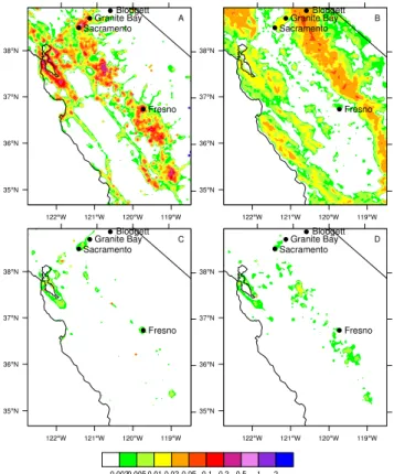
cate-Fig. 1. Primary, present-day emissions (mol s−1)for four VOC
categories: (a)anthropogenic,(b)biogenic, and(c)aldehyde and (d)other oxygenated VOC. All figures display the average emission flux at 09:00 LT.
gories each for olefins (OLE1, OLE2) and aromatics (ARO1, ARO2). Model anthropogenic species are listed in Table 1 along with average morning contributions to total VOC re-activity. The modeled anthropogenic VOC category repre-sents the total amount of anthropogenic hydrocarbon primary emissions (spatial distribution shown in Fig. 1a) based on gridded emission inventory data supplied by the California Air Resources Board and modified by Marr et al. (2002) and Harley et al. (2005). Emissions of anthropogenic VOC are dominated by higher alkanes (ALK3-ALK5) and ethene.
Table 1. Average morning modeled ROH,VOCfor four VOC categories: anthropogenic, biogenic, aldehydes, and other oxygenated VOC. kOHvalues for anthropogenic VOC reactions (alkanes, olefins and aromatics) are in ppm−1min−1(Carter, 2000).
CMAQ Category Description Sacramento Fresno Granite Bay Blodgett Forest
Anthropogenic 2.635 1.988 1.590 0.146
ETHENE Ethene 0.516 0.330 0.326 0.036
ALK1 alkanes/non-aromatics, 200<kOH<500 0.015 0.046 0.017 0.004
ALK2 alkanes/non-aromatics, 500<kOH<2500 0.028 0.028 0.019 0.004
ALK3 alkanes/non-aromatics, 2500<kOH<5000 0.088 0.133 0.066 0.005
ALK4 alkanes/non-aromatics,5000<kOH<10 000 0.231 0.238 0.177 0.010
ALK5 alkanes/non-aromatics,kOH>10 000 0.285 0.282 0.196 0.007
OLE1 Alkenes withkOH<70 000, usu. terminal alkenes 0.506 0.230 0.305 0.036
OLE2 Alkenes withkOH>70 000, usu. internal or disubstituted alkenes 0.364 0.215 0.017 0.016
ARO1 Aromatics withkOH<20 000, usu. toluene and monoalkyl benzenes 0.131 0.104 0.101 0.011
ARO2 Aromatics withkOH>20 000, usu. xylenes and polyalkyl benzenes 0.546 0.429 0.384 0.019
Biogenic 1.893 0.392 0.318 6.124
ISOP Isoprene 1.473 0.349 0.240 2.570
TRP Biogenic alkenes less isoprene 0.356 0.046 0.022 0.359
MBO 2-methyl-3-buten-2-ol 0.236 0.049 0.037 2.885
Aldehydes 1.642 1.492 1.506 1.071
HCHO Formaldehyde 0.908 0.629 0.862 0.411
CCHO Acetaldehyde and glycolaldehyde 0.354 0.444 0.323 0.309
RCHO Lumped C3+ aldehydes 0.321 0.353 0.270 0.321
BALD Aromatic aldehydes 0.012 0.010 0.011 0.001
GLY Glyoxal 0.014 0.015 0.012 0.003
MGLY Methyl glyoxal & higher a-dicarbonyls 0.033 0.041 0.028 0.026
Other Oxygenated 0.399 0.338 0.174 0.413
ACET Acetone 0.003 0.008 0.002 0.004
MEK Ketones withkOH<5×10⁻¹²cm3molec−1s−1 0.010 0.029 0.009 0.008
MEOH Methanol 0.002 0.003 0.001 0.001
PHEN Phenol 0.0003 0.0002 0.0001 0.00002
CRES Cresols 0.010 0.010 0.009 0.001
MVK Unsaturated ketones 0.049 0.043 0.029 0.070
MACR Methacrolein 0.154 0.050 0.026 0.105
IPRD Unsaturated aldehydes other than acrolein and methacrolein 0.105 0.076 0.043 0.153 PROD2 Ketones withkOH<5×10⁻¹²cm3molec−1s−1 0.066 0.119 0.055 0.071
The third category, aldehydes, includes primary emissions sources as well as the secondary oxidation products of an-thropogenic and biogenic VOC. In the model, we consider six aldehyde categories, detailed in Table 1. Primary an-thropogenic emissions of aldehydes in the model are shown in Fig. 1c and include formaldehyde (HCHO), acetalde-hyde (CCHO), benzaldeacetalde-hyde, other C3+ aldeacetalde-hydes (RCHO), glyoxal (GLY) and methylglyoxal (MGLY). Primary urban emissions of aldehydes are dominated by HCHO and CCHO. The fourth category, other oxygenated VOC, includes nine model categories (Table 1). Primary emissions (Fig. 1d) include acetone, C4+ ketones (MEK), phenol, cresol and methanol, and the dominant emissions of oxygenated species in urban regions are MEK, methanol and acetone, although aldehyde and other oxygenated VOC emissions tend to be 1–2 orders of magnitude less than anthropogenic or bio-genic VOC emissions. The primary emissions of
aldehy-des and other oxygenated VOC in the model are solely an-thropogenic and are located near urban and industrial ar-eas. These anthropogenically-emitted species can also be produced in the atmosphere as secondary products from the oxidation of anthropogenic and biogenic VOC. Additional other oxygenated VOC that are a result of atmospheric oxi-dation only include PROD2 (a lumped oxygenated VOC that represents secondary products from both biogenic and an-thropogenic VOC oxidation), MVK, MACR, and IPRD (re-sulting primarily from biogenic VOC oxidation).
Table 2. Measured chemical species in each of the four VOC categories, ranked in order of reaction rate. List of species used to esti-mate calculated ROH,VOCat each of the following sampling locations: Sacramento PAMS (2000 data), Blodgett Forest Research Station (22/07/2001–19/09/2001), and Granite Bay (16/07/2001–17/09/2001), with average afternoon concentrations (ppb). CMAQ lumped cate-gories for each measured species are indicated for comparison with modeled ROH,VOC.
VOC Categories and kaOH×10−12(cm3molec−1s−1) PAMSb Blodgettb Granite Bayb CMAQ Chemical Species
Anthropogenic VOC
1,3-butadiene 68.3 0.026 OLE2
trans-2-pentene 67.0 0.107 0.016 OLE2
trans-2-butene 66.0 0.130 0.009 OLE2
cis-2-pentene 65.0 0.099 0.007 OLE2
2-methyl-1-butene 60.7 0.019 OLE2
styrene 58.0 0.089 OLE2
cis-2-butene 57.9 0.121 OLE2
1,3,5-trimethylbenzene 57.5 0.836 ARO2
cyclopentene 57.0 0.004 OLE2
2-methylpropene (isobutene) 52.8 0.027 0.081 OLE2
1,2,4-trimethylbenzene 37.5 0.084 ARO2
1,2,3-trimethylbenzene 32.7 0.174 ARO2
1-butene 32.2 0.144 0.038 0.034 OLE1
1-pentene 31.4 0.118 0.036 OLE1
propene 30.0 1.029 0.367 OLE1
m-xylene 23.6 1.792c 0.240 ARO2
m-ethyltoluene 17.1 0.018 ARO2
p-xylene 14.3 1.792c 0.133 ARO2
m-diethylbenzene 14.2 ARO2
o-xylene 13.7 0.296 0.123 ARO2
o-ethyltoluene 12.3 0.184 ARO2
n-undecane 12.9 2.021 ALK5
p-ethyltoluene 11.4 0.073 ARO2
n-decane 11.2 0.070 ALK5
methylcyclohexane 10.0 0.170 ALK5
n-nonane 9.91 0.063 ALK5
n-octane 8.60 0.086 ALK5
3-methylheptane 8.56 0.073 ALK5
2-methylheptane 8.28 0.903 ALK5
p-diethylbenzene 8.11 0.097 ARO2
3-methylhexane 7.16 0.232 ALK5
ethylbenzene 7.10 0.497 0.021 0.080 ARO1
cyclohexane 7.10 0.193 ALK5
2,3,4-trimethylpentane 7.10 0.010 ALK5
n-heptane 6.98 0.208 0.243 ALK5
methylcyclopentane 6.80d 0.353 ALK4
isopropylbenzene 6.50 0.085 ARO1
toluene 6.40 0.340 0.085 0.488 ARO1
2,3-dimethylpentane 6.10 0.119 ALK5
propyne (methyl acetylene) 5.90 0.022 0.022 ALK4
2,3-dimethylbutane 5.75 0.147 ALK4
n-propylbenzene 5.70 0.187 ARO1
in the ALK3 category (Table 2) despite the oxygenated na-ture of the compound. However, MTBE and other similar compounds tend to have low reactivity and comprise a small portion of the total anthropogenic VOC emissions.
Table 2.Continued.
Anthropogenic VOC, cont.
3-methylpentane 5.40 0.294 0.011 0.351e ALK4
n-hexane 5.40 0.276 0.015 0.135 ALK4
3-methyl-1-butene 5.32 0.016 OLE1
2-methylpentane 5.30 0.626 0.022 0.351e ALK4
2-methylhexane 5.10 0.154 ALK5
2,4-dimethylpentane 5.00 0.091 ALK4
cyclopentane 4.92 0.122 0.041 ALK4
n-pentane 3.91 0.567 0.038 0.259 ALK4
isopentane 3.70 1.579 0.067 0.665 ALK4
methyl tert-butyl ether 2.96 1.943 ALK3
2,2-dimethylbutane 2.34 0.112 ALK4
n-butane 2.34 0.779 0.080 0.443 ALK3
isobutane 2.15 0.498 0.045 0.300 ALK3
benzene 1.17 0.136 0.227 0.152 BENZ
propane 1.07 2.406 1.489 ALK2
acetylene 0.78 1.587 ALK2
ethene 0.236 1.648 ETHE
ethane 0.236 2.017 ALK1
2,2-dimethylpropane 0.0000179 0.005 ALK2
Biogenic VOC
d-limonene 171.0 0.031 TRP1
isoprene 103.0 1.521 0.262 0.516 ISOP
3-carene 88.0 0.010 TRP1
b-pinene 80.5 0.125 TRP1
methylbutenol 64.0 1.135 MBO
a-pinene 55.1 0.123 0.035 TRP1
Aldehydes
hexanal 31.7f 0.276 RCHO
pentanal 29.9f 0.064 0.118 RCHO
acetaldehyde 15.8 1.398 1.386 1.417 CCHO
formaldehyde 9.20g 2.658 HCHO
Oxygenated VOC
3-methylfuran 93.5h 0.009
methacrolein 35.0 0.289 0.213 MACR
methyl vinyl ketone 18.8 0.331 0.309 MVK
ethanol 3.27 2.257 ALK3
methyl ethyl ketone 1.15 0.213 MEK
methanol 0.94 10.735 7.467 MEOH
acetone 0.22 2.507 2.911 ACET
ak
OHvalues based on Atkinson (1994) unless noted otherwise.
bAverage AM (06:00–08:00 a.m. local time) concentrations over the sampling period, in ppb. PAMS data listed is an average of the four
sites in the Sacramento metropolitan area.
cPAMS stations report co-eluting m- and p-xylene as a single sum, therefore concentrations shown here are the sum of these two isomers. dEstimated from Kwok and Atkinson (1995).
eGranite Bay measurements include total methylpentanes, here listed as 2-methylpentane. fPapagni et al. (2000)
alcohols, ketones, esters, and ethers (Kesselmeier and Staudt, 1999; Schade and Goldstein, 2001). However, measurements and modeling efforts have yet to thoroughly quantify these species on the scale needed for regional emissions modeling, and they are not included in our biogenic VOC emissions in-ventory.
2.3 Ground-based measurements
We utilize ground-based measurements at four locations in central California (marked in Fig. 1). For two locations, Sacramento and Fresno, we use observations from the Pho-tochemical Assessment Monitoring Stations (PAMS) net-work. At eleven sites in four different geographic regions in California (in Sacramento, Fresno, Kern and Madera coun-ties), ground-based O3, CO, NOx, and VOC measurements have been collected from 1994 to the present. The VOC dataset consists of a long-term record of 55 VOC species (see Table 2) collected at 3-h intervals, including alkanes, alkenes and aromatics (data available at www.epa.gov/air/ oaqps/pams). This dataset predominantly reflects the anthro-pogenic VOC category as defined in Sect. 2.2, with isoprene measurements at these locations representing only a portion of the biogenic VOC category. Selected PAMS sites measure a suite of carbonyl species, including formaldehyde and ac-etaldehyde, and we include these measurements when avail-able. Here, we include concurrent VOC and NOxdata from the summer of 2000 for the Sacramento (four measurement sites) and Fresno (three measurement sites) metropolitan ar-eas. While the PAMS data have been known to have several artifacts in the hydrocarbon and aldehyde samples due to the nature of canister samples (McClenney et al., 2002), we uti-lize this data here in the absence of in-situ VOC sampling in the region and note that these results should be reviewed with caution with respect to the carbonyl species.
A third sampling location, Granite Bay, was established in the summer of 2001 to evaluate the transport of pollutants at the eastern edge and downwind of Sacramento. NO2was measured from 19/07/2001–15/09/2001, and NOx concentra-tions are estimated from NO2 photolysis, measured ozone, and modeled RO2(Cleary et al., 2005). A suite of VOC was measured at the same location, including 28 anthropogenic, 4 biogenic, 4 aldehydes and 7 other oxygenated VOC (Millet et al., 2005). As shown in Table 2, measurements in the an-thropogenic, biogenic and other oxygenated VOC categories represent a significant portion of the modeled VOC reactiv-ity, while the aldehyde category is missing the important con-tribution of HCHO.
The fourth location, Blodgett Forest Research Station, is located in the Sierra Nevada mountains approximately 75 km ENE of Sacramento, and represents a rural site where con-centrations and fluxes of biogenic VOC compounds have been measured during summer months since 1997 (e.g., Lamanna and Goldstein, 1999). Additional VOC concen-trations were measured in 2001 in conjunction with Granite
Bay measurements. These include a limited number of an-thropogenic (10 species), aldehydes (2 species), other oxy-genated VOC (4 species), and the dominant biogenic VOC (4 species) (Table 2). While the number of VOC species measured at Blodgett is small compared to other sites, the measurements comprise the major biogenic species emitted and are likely representative of VOC chemistry at the site. Additionally, NOxhas been measured at the site (Day et al., 2003, 2007), and data were filtered for concurrent NOxand VOC measurements.
2.4 ROH,totaland ROH,VOCdefinitions
Here, we define the total OH reactivity (ROH,total, s−1)as OH loss with the following species: CO, CH4, NO2, an-thropogenic VOC, biogenic VOC, aldehydes, and other oxy-genated VOC:
ROH,total=kCO+OH[CO]+kCH4+OH[CH4]+kNO2+OH[NO2]
+ X
n=1,navoc
kn+OHaVOCn,meas+ X
n=1,nbvoc
kn+OHbVOCn,meas
+ X
n=1,naldvoc
kn+OHaldVOCn,meas+ X
n=1,noxvoc
kn+OHoxVOCn,meas
(1) where navoc (nbvoc, naldvoc, noxvoc) is the number of anthropogenic (biogenic, aldehyde, other oxygenated) VOC species,kn+OHis the rate coefficient (cm3molecules−1s−1) and [VOCn,meas] is the measured VOC concentration. VOC reactivity (ROH,VOC)is calculated from the four VOC cate-gories only:
ROH,VOC= X
n=1,navoc
kn+OHaVOCn,meas+ X
n=1,nbvoc
kn+OHbVOCn,meas
+ X
n=1,naldvoc
kn+OHaldVOCn,meas+ X
n=1,noxvoc
kn+OHoxVOCn,meas
(2) Reactivities are calculated from ground-based CO, CH4, NO2 and VOC concentrations and kinetic rate coefficients calculated from measured temperature and pressure (Ta-ble 2).
Modeled reactivities are determined from integrated reac-tion rates calculated by CMAQ, which estimates the loss rate of each species that reacts with OH integrated over each hour:
OHloss(t+1t )=OHloss(t )+ t+1t
Z
t
kn+OH[OH][n]dt (3)
VOCloss(t+1t )=VOCloss(t )+ t+1t
Z
t
kn+OH[OH][VOC]dt (4)
Fig. 2.Measured (gray circles) versus modeled (black crosses) cumulative distribution functions for(a)Sacramento NOx,(b)Fresno NOx, (c)Granite Bay NOx,(d)Blodgett NOx, and(e)Sacramento ROH,VOC,(f)Fresno ROH,VOC,(g)Granite Bay ROH,VOC, and(h)Blodgett ROH,VOC.
nwith the OH radical, and [OH] and [n] represent concen-trations at timet (Byun and Ching, 1999). For OH loss, n
includes CO, CH4, NO2, and the four VOC categories. For VOC loss, n includes only the four VOC categories. This representation provides an accurate method of assessing the loss rates of each species with OH. In order to compare the model loss rates with observations in California and else-where, we assume that the modeled OH concentrations are relatively stable over the timescale of the hour of integration and calculate the modeled OH and VOC reactivity as:
ROH,total= OHloss
[OH] (5)
ROH,VOC=
VOCloss
[OH] (6)
For ROH,VOC, we calculate this quantity as the sum of indi-vidual species for each of the four VOC categories, consider-ing only daytime modeled and calculated reactivity calcula-tions, when OH dominates radical reactivity with VOC. We note the definitions of ROH,totaland ROH,VOCare closely con-nected, as changes in concentrations of CO, NO2and CH4 will impact OH concentrations and in turn the rate of VOC reactions. Therefore, ROH,VOCis a subset of ROH,total.
3 Results and discussion
Re-Fig. 3.Measured (gray circles) versus modeled (black crosses) cumulative distribution functions for four Sacramento locations(a)upwind location, Elk Grove NOx,(b)near-urban location, Sacramento Del Paso Manor NOx,(c)near-urban location, Natomas Airport NOx,(d) downwind location, Folsom NOx,(e)Elk Grove RAVOC,(f)Sacramento Del Paso Manor RAVOC,(g)Natomas Airport RAVOC, and(h) Folsom RAVOC.
activities calculated from Granite Bay and Blodgett forest are based on measurements conducted during 2001.
In Sacramento during the daytime, the NOxCDF (Fig. 2a) indicates that the model predicts less NOx than observed at the lower end of the NOx concentrations, while the Fresno results indicate that the model predicts less NOx at all times and over the full width of the distribution (Fig. 2b). Mean daytime NOxconcentrations are less than those mea-sured (Sacramento meamea-sured daytime mean NOx=10 ppb, modeled mean NOx=7 ppb; Fresno measured daytime mean NOx=23.5 ppb, modeled mean NOx=5 ppb). A portion of this daytime discrepancy is likely due to the NO2 chemi-luminescence measurement technique employed at the EPA PAMS monitoring locations. This technique is well known to include PAN and other higher oxides of nitrogen in the re-ported NO2and thus to have a high bias (e.g., Winer et al., 1974). Recent measurements using current commercial im-plementations of the technique side by side with instruments that specifically measure NO2show that high biases of 20– 50% occur routinely (Dunlea et al., 2007; Steinbacher et al., 2007).
Other possibilities for measured and modeled discrepan-cies include the vertical averaging technique, the impacts of dilution due to meteorological parameters, and the location of urban monitoring stations. Vertical averaging is not a
sig-nificant factor, as comparisons of concentrations in the sur-face layer only (sursur-face to 20 m) only impact the top 90% of the distribution, and indicate that the model still underesti-mates the majority of the distribution in urban locations (re-sults not shown). Because measured and modeled boundary layer heights are similar in Sacramento (daily maxima ap-proximately 500–600 m) and Fresno (daily maxima approx-imately 600–800 m) during the simulation time period and daytime wind speeds and wind directions agree fairly well (Wilczak et al., 2004; data available at http://www.etl.noaa. gov/programs/modeling/ccos/data/), dilution is not likely a strong factor in the differences in the measured and modeled distribution functions.
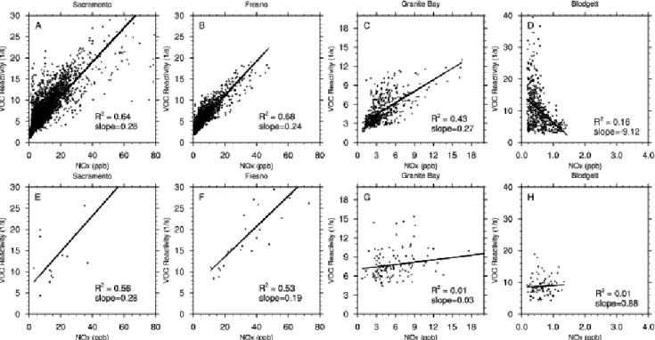
Fig. 4.Total ROH,VOC(s−1)as a function of NOxconcentrations (ppb), as modeled(a–d)and measured(e–h)in four locations: Sacramento (a, e), Fresno (b, f), Granite Bay (c, g), and Blodgett Forest (d, h). See Table 1 for VOC included in these calculations.
immediate vicinity (Fig. 3). The four PAMS sites represent upwind (Type 1 sites), near urban (Type 2 sites), and down-wind locations (Type 3 sites). Elk Grove (Fig. 3a and e) cor-responds to an upwind location, while Sacramento Del Paso (Fig. 3b and f) and Natomas Airport (Fig. 3c and g) repre-sent locations near maximum emissions in the urban area, and Folsom (Fig. 3d and h) is located downwind of the ur-ban area and near the location of maximum ozone. The site locations relative to the urban area (e.g., upwind or down-wind) do not have a strong impact on the NOx and RAVOC CDFs. In the upwind location of Elk Grove, the model cap-tures the median NOx accurately but does not capture the minimum or the maximum NOxconcentrations. At the Del Paso urban site (Fig. 3b) the model accurately reproduces the measured CDF while at Natomas Airport (a second ur-ban location) the model consistently predicts less NOxthan observed. At the downwind site, Folsom, the model predicts less NOxand RAVOCthan observed.
Because these factors do not show a significant impact, this suggests that the discrepancy between measured and modeled NOx distributions are due to differences in an-thropogenic emissions. Similar to the NOxcomparisons in Sacramento and Fresno, modeled ROH,VOCis also less than observed throughout the entire distribution (Fig. 2e and f), suggesting an underestimate in modeled anthropogenic VOC emissions as well. Overall, the CDFs indicate that the model under estimates emissions of NOxand anthropogenic VOC throughout the Sacramento and Fresno regions.
At Granite Bay, a suburban Sacramento location at the same longitude as Folsom but located approximately 12 km north, a different NO2measurement technique is used (Laser Induced Fluorescence (LIF); Thornton et al., 2000; Cleary et al., 2002). Here, the CDFs indicate that observed NOx con-centrations are fairly well represented by the model in the bottom 50% of the distribution (similar mode, with modeled median = 3.3 ppb and measured median = 4.9 ppb), with in-creasing differences at the high end (model less than observa-tions, Fig. 2c). A similar NOxdistribution mode is predicted by the model at Granite Bay as at Folsom, but measured NOx is lower at Granite Bay than at Folsom. This fact indicates that in the Sacramento region, the overestimate of NO2by the PAMS monitoring network is one of the dominant sources of the model-measurement difference, but that also some un-derestimate of emissions by the model is also contributing. For the ROH,VOC distribution (Fig. 2g), the model predicts less ROH,VOCthan indicated by measurements, particularly at the lower end of the distribution. This is due in part to the greater contribution of biogenic VOC to calculated ROH,VOC than predicted by the model (see further discussion below in Sect. 3.3).
of individual VOC categories to ROH,totaland ROH,VOCis in-cluded in Sects. 3.3 and 3.4 below.
3.2 The relationship between ROH,VOCand NOx
Another approach to evaluating modeled VOC is to com-pare the functional relationships of ROH,VOC versus NOx with observations (Fig. 4). In Sacramento (Fig. 4a and e), the measurements and model both span a similar range of NOx concentrations (up to 80 ppb) and ROH,VOC (up to 30 s−1). The increase in ROH,VOC with NOx predicted by the model is close to the observations (slope of 0.28 for both the model and measurements with similarR2values), how-ever the sparse data in Sacramento limits the robustness of this result. In Fresno (Fig. 4b and f), NOx concentrations and ROH,VOC range up to 60 ppb and 30 s−1, respectively, for both measured and modeled data, with similar slopes of approximately 0.2 s−1/ppb. This indicates increasing model emissions to match observed CDFs would need to be from a source that emits NOxand ROH,VOCin the same proportion as observed. Because biogenic VOC emissions in Fresno are relatively small, this suggests an anthropogenic source that co-emits NOxand VOC, including some industrial processes and motor vehicle emissions. Another possibility in the Cen-tral Valley is agricultural emissions, which can also emit both NOxand VOC. Our simulations do not include agricultural NOx emissions, and only traditional biogenic VOC emis-sions (isoprene and monoterpenes) from crops are included in the biogenic inventory despite knowledge that crops emit a wide variety of biogenic oxygenated VOC (e.g., Kesselmeier and Staudt, 1999).
At Granite Bay (Fig. 4c and g), daytime measured and modeled NOx concentrations range from 0-18 ppb and ROH,VOCranges from 0–15 s−1. Here the model predicts a stronger linear trend of NOxand ROH,VOC(slope=0.43 and R2=0.27), while the measurements indicate little to no trend (slope=0.03 andR2=0.01). At Blodgett Forest, NOx concen-trations are low (<2 ppb) at this site in both the model and the measurements. The model predicts ROH,VOCapproximately twice that of the measurements and shows that ROH,VOCand NOx are anti-correlated, which is expected at a rural loca-tion. Further discussion of these differences is presented in Sects. 3.3 and 3.4.
3.3 The diurnal cycle of ROH,total
We next look at the contributions of individual species to modeled ROH,total over the daytime diurnal cycle (Fig. 5). During the daytime, VOC play a dominant role while NO2 loss dominates at night. In the urban locations (Sacramento and Fresno; Fig. 5a and b), the dominant daytime ROH,total is due to anthropogenic VOC and aldehydes. For these two VOC categories, ROH,totalpeaks during the early morn-ing rush hour, and a rise in the contribution of the sec-ondary VOC categories (aldehydes and other oxygenated
Fig. 5. Average daytime (LT) modeled diurnal cycle of ROH,total
(black dashed line) and reactivities of six species at four locations: (a)Sacramento,(b)Fresno,(c)Granite Bay, and(d)Blodgett For-est. Species contributing to ROH,totalinclude NO2(brown solid), CO (red solid), anthropogenic VOC (black solid), biogenic VOC (green solid), aldehydes (blue solid), and other oxygenated VOC (orange solid). CH4 (not shown) contributes a constant value of 0.3 s−1to ROH.
VOC species) occurs about an hour or two later. In Sacra-mento, biogenic VOC play a role equal to aldehydes in the model, while biogenic VOC are of minor importance in Fresno. The remaining three categories (CO, CH4 and other oxygenated VOC) tend to contribute less than 1 s−1to ROH,total.
In Granite Bay (Fig. 5c), ROH,total also peaks during the morning rush hour when photochemistry is accelerated, pre-dominantly due to biogenic VOC. Biogenic ROH,VOC also peaks at 6 s−1, a value greater than that of anthropogenic VOC or aldehydes. We note that the model does not repro-duce the second diurnal peak in reactivity observed at Gran-ite Bay (Murphy et al., 2006b), and this could be due to the lack of afternoon emissions in the model (discussed below with reference to Fig. 6) or poor representation of mixing and chemistry during the evening boundary layer transition. Ad-ditionally, the diurnal cycle of modeled biogenic ROH,VOC does not reflect the emissions pattern, which peaks at mid-day due to temperature and radiation patterns. The accuracy of the model related to this peak in biogenic ROH,VOCis dis-cussed in greater detail in the discussion below.
Fig. 6. Modeled and calculated percent contribution to ROH,total (s−1)for the four central California locations during(a)morning hours (6–8 a.m. local time) and(b)afternoon hours (1–3 p.m. local time). ROH,totalincludes contributions from four VOC categories (anthropogenic, biogenic, aldehydes, and other oxygenated VOC), CO, CH4and NO2. Calculated contributions explained in the text and Tables 1 and 2. ROH,totalfor each location is noted at the lower right hand of each pie chart. Hatched regions indicate estimated contributions.
ROH,total=17 s−1, corresponding to the time of maximum bio-genic VOC flux. Oxidation products of these biobio-genic VOC (included in the aldehyde and other oxygenated VOC cate-gories) are the second greatest contributors, reaching a max-imum approximately one to two hours after the biogenic ROH,VOCpeak. In comparison with calculated diurnal vari-ation in reactivity at Blodgett (Murphy et al., 2006b), the model produces a much stronger midday peak in reactiv-ity (17 s−1) compared to an average afternoon reactivity ob-served by Murphy et al. (2006b) of 4–5 s−1. Because the biogenic VOC model is tuned to Blodgett measurements, modeled fluxes of well-characterized biogenic VOC such as methylbutenol compare well with measurements (Steiner et al., 2007), and similar chemical species are included in the measurements and model due to the large amount of data available for Blodgett forest. Therefore, the differences are likely due to errors in the model representation of oxidation rates or mixing rates.
Measurements at the PAMS sites are insufficient to assess the full modeled ROH,total diurnal cycle, but there is suffi-cient data to compare the model and measurements during the morning and afternoon time periods. In some cases, we estimate the contribution of important species that are not included in the measurements. The contribution of CH4 to ROH,total is estimated for both modeled and calculated ROH,total based on a concentration of 1800 ppbv. For the
PAMS measurement sites (Sacramento and Fresno), the mea-surements include a large number of anthropogenic hydro-carbons, accounting for many of the reactive species and ac-counting for a large portion of the modeled lumped anthro-pogenic categories. However, some important biogenic com-pounds (terpenes and MBO), aldehyde (RCHO), and other oxygenated VOC that can yield a significant contribution to the total are not measured (see Table 1). For these species, we use model reactivities to estimate their contribution to ROH,total, as indicated by the hatched regions of Fig. 6. For Granite Bay and Blodgett, the anthropogenic measurements are not as complete as those provided by the PAMS sta-tions. Therefore, we include model estimates of the top two contributors to anthropogenic ROH,VOC(ethene and ARO2), which are not measured at these locations. We also include model estimates of two important aldehydes (HCHO and RCHO), which are unmeasured yet can contribute signifi-cantly to ROH,VOC. The detailed measurements of biogenic and other oxygenated species at Granite Bay and Blodgett include most of the important reactive species for these two categories (Table 2).
the model (RCHO) indicates that the aldehyde measurements at this location (HCHO and CCHO) are fairly representa-tive of the modeled aldehyde species at this location. Other oxygenated VOC measurements are not available for Sacra-mento, although they contribute a relatively small fraction in the model (4%). During the afternoon (Fig. 6b), incomplete measurements do not allow for a comparison, but the mod-eled NO2fraction increases along with a decrease in the pri-mary emissions reactivity (anthropogenic and biogenic) and an increase in the secondary VOC reactivity (aldehydes and other oxygenated VOC).
In the morning in Fresno (Fig. 6a), the model underesti-mates ROH,totalby a factor of 2–3 compared to ground-based estimates. A large portion of this difference is due to NO2 and, as in Sacramento, the modeled contribution (18%) is about half that of the calculated portion (38%). Calculated and modeled CO and CH4also have similar contributions as in Sacramento (11–14% and 2–3%, respectively). VOC con-tributions to ROH,totalare about 50% based on measurements and about 60% in the model. Anthropogenic VOC contribu-tions to ROH,total are similar in the calculated and modeled results (∼30%), while the model predicts slightly greater biogenic (6% modeled vs. 4% calculated), aldehyde (22% modeled vs. 15% calculated), and other oxygenated VOC (5% in the model) contributions. In general, missing mea-surements of biogenic (terpenes and MBO; green hatched regions) and aldehydes (RCHO; blue hatched regions), as described above, contributed very little to total estimates of biogenic and aldehyde species. Overall in the morning at Fresno, the relative contributions of different types of VOC to ROH,totalare similar in the model and observations. This fact coupled with the observation that total reactivity and NOx are both low by about the same amount suggests that the model emissions should be substantially increased for both NOx and VOC in this region. VOC measurements are not available during the afternoon at Fresno, but similar to Sacra-mento, the model predicts a smaller contribution of primary VOC reactivity while secondary VOC (aldehydes and other oxygenated VOC) reactivity increases.
Direct measurements of ROH,totalhave been performed in several other urban locations in North America. In Nashville, ROH,total was calculated in the range of 5–25 s−1, with a median value of 11 s−1 (Kovacs et al., 2003); measure-ments range from 15–25 s−1 with a median of 19 s−1 in New York City (Ren et al., 2003). Other studies have estimated ROH,total from VOC and NOx measurements to range from 2–20s−1 (median=∼4 s−1) for Nashville, and 1.5–10s−1(median=∼4 s−1)for New York City (Kleinman et al., 2005). The ROH,totalwe estimate from Sacramento and Fresno (6–20 s−1)are consistent with those of other urban areas in the United States.
At Granite Bay (Fig. 6a), the calculated (10.6 s−1) and modeled (10.2 s−1) morning ROH,total is very similar. As with Sacramento and Fresno, however, the model predicts a much smaller contribution of NO2to the ROH,total, the
mea-surements show that the ROH,totaldue to NO2is 2.6 s−1while the model calculates 0.8 s−1. Anthropogenic VOC compo-nents agree well in the morning (about 16% in the measure-ments and 13% in the model), and including additional an-thropogenic VOC (black hatched regions) does not make a significant impact on ROH,VOC. The model predicts a greater fraction of the total reactivity is biogenic VOC,∼50% com-pared to the 20% in the measurements. This suggests that the morning biogenic VOC reactivity is much larger than that observed. Calculated and modeled aldehyde reactivi-ties are similar, contributing about 23% and 17% to ROH, respectively. Calculated CCHO reactivity at Granite Bay is greater than that predicted by the model, leading to a greater aldehyde reactivity based on measurements. In the after-noon at Granite Bay (Fig. 6b), the model predicts ROH,total that is a factor of two smaller than the measurements. The greatest discrepancies for the calculated and modeled reac-tivities at Granite Bay can be attributed to NO2, biogenic VOC, and aldehyde components. Again NO2is underesti-mated, although not as significantly as in the morning hours. Aldehyde chemistry in the model tends to follow the changes in anthropogenic and biogenic reactivity (increases as the anthropogenic and biogenic reactivity decreases), but this is not reflected in the measurements. The model predicts more biogenic reactivity than aldehyde ROH,VOCin the morn-ing, while the measurements indicate that aldehyde ROH,VOC dominates over biogenic ROH,VOC.
At Blodgett Forest in the morning (Fig. 6a), calculated and modeled ROH,total values are within 40% (6.8 s−1 cal-culated, 9.4 s−1modeled). Contributions from NO
2(1-3%), CO (4–12%), and CH4 (3–4%) are small compared to that from VOC, which contribute about 80% based on measure-ments and 90% in the model. Anthropogenic VOC plays a small role in ROH,total (2–3%). At Blodgett, the differ-ences in ROH,total stem primarily from discrepancies in the biogenic category. The model predicts about 75% of the ROH,total is due to biogenic VOC in the morning, while the measurements show this fraction is about 50%. In the after-noon (Fig. 5b), calculated and modeled ROH,totaland relative VOC contributions are within 10% of each other, again with an overestimate of biogenic reactivity in the model compared to observations. One possible reason for this difference could be due to the biogenic emissions model, which predicts pri-mary isoprene fluxes from Blodgett forest that are not ob-served at the site. These emissions, which are nearly equal to MBO emissions, could be contributing to the higher re-activity in the model. Another possibility is that fast chem-istry within the forest canopy could react away many of the highly reactive terpenes and this fast chemistry cannot be re-produced by the model. Both of these factors could con-tribute to the over prediction of modeled ROH,VOC.
mod-Fig. 7. Speciated ROH,VOC(s−1)as a function of NOx concen-trations (ppb) in Sacramento, as(a)modeled and (b)calculated. The contribution of the four VOC categories to the ROH,VOC, in-cluding anthropogenic VOC (black), biogenic VOC (green), alde-hydes (blue), and other oxygenated VOC (orange). For the calcu-lated Sacramento ROH,VOC, biogenic ROH,VOCis based on iso-prene concentrations only, and aldehydes are based on HCHO and CCHO concentrations only. See Table 1 for a full list of VOC species included in each category.
eled and observed VOC contributions to ROH,totalin the two urban locations show that NO2and anthropogenic VOC are the two largest factors. The main categories of VOC con-tribution to ROH,totalin urban areas are anthropogenic VOC (∼28%), followed by aldehydes (17–22%), biogenic VOC (6–20%), and other oxygenated VOC (4–6%). Modeled bio-genic VOC contribute more to OH reactivity in Sacramento (20%) than Fresno (6%), and this is reflected in the measure-ments.
At Granite Bay, the model and measurements agree well on ROH,total in the morning but not in the afternoon, while the opposite is true at Blodgett Forest. In both locations, the discrepancies are due to the relative contributions of aldehy-des and biogenic VOC. At Granite Bay, modeled biogenic VOC is greater than calculated in the morning, but the con-verse is true in the afternoon. At Blodgett Forest, the model consistently predicts greater biogenic VOC than that calcu-lated from measurements. These differences are indicative of errors in chemistry, as we have shown the emissions are consistent with observations.
3.4 The relationship between speciated ROH,VOCand NOx More insight into where the model is accurately describing the relationships between NOx and VOC reactivity can be found by comparing each of the four VOC categories ver-sus NOx (Fig. 7). In the urban locations, we expect that anthropogenic VOC and NOxwill be positively correlated, as both emissions have primary sources from transportation and chemical removal largely occurs downwind. In Sacra-mento, the slopes of correlation of anthropogenic VOC re-activity with NOxare 0.15 s−1/ppb NOxfor the observations and 0.19 s−1/ppb NOxfor the model. We note that some of the difference in slope could be due to the positive bias in the
Fig. 8. Measured (gray circles) versus modeled (black crosses)
cumulative distribution functions for(a)Sacramento odd oxygen (O3+NO2)and(b)Fresno odd oxygen. Ozone and NO2data from PAMS stations represents daytime data during the time period of the simulation (29/07/2000–03/08/2000).
PAMS NO2as discussed in Sect. 3.1. There are no signifi-cant correlations of NOxand the other categories of VOC in the observations or the model.
3.5 Implications for ozone chemistry
Based on the above comparisons between measured and modeled urban chemistry, the under estimation of NOxand VOC emissions inventories are notable and likely have im-plications for ozone prediction in central California. Our prior central California ozone study (Steiner et al., 2006) compared modeled afternoon ozone concentrations versus ground-based observations, and found that the near-surface ozone daily maxima were reproduced by in the model in the central Valley. In the Sacramento region, however, modeled ozone maximum concentrations were about 10–20 ppb less than those observed, and this discrepancy was attributed to poor meteorological representation of upslope flow along the Sierra. In Fresno, measured concentrations of ozone show similar maxima to those modeled (90–100 ppb). Results from this study indicate that inaccurate emissions inventories could also contribute to these differences in ozone concentra-tions.
are based on ozone concentrations and not local ozone pro-duction, it is impossible to discern the difference between lo-cally produced and transported ozone at this time. However, this does suggest that merely increasing NOxand VOC emis-sions to address the emission estimate discrepancies may not improve ozone prediction in central California.
3.6 Present day and future spatial distributions of ROH,VOC Over the model domain, ROH,VOC reaches up to 16 s−1 in the morning hours and is greatest near urban areas and re-gions with high biogenic VOC emissions (Fig. 9a). ROH,VOC outside regions with high anthropogenic and biogenic VOC emissions tend to be low (<4 s−1). The contribution of each VOC category to total modeled reactivity varies with emis-sions geography. Anthropogenic and biogenic VOC reactiv-ities are located near emission sources (Fig. 9b and c), with anthropogenic ROH,VOC occurring near urban centers and biogenic ROH,VOCdominating in the mountainous and veg-etated regions of the domain. However, an interesting point in this simulation is the importance of aldehyde and other oxygenated species with respect to ROH,VOCthroughout the model domain (Fig. 9d). Overall, the aldehyde and other oxygenated ROH,VOCaccounts for at least 40% of ROH,VOC. In agricultural regions of the Central Valley, where measure-ments are unavailable, the oxygenated VOC fraction rep-resents up to 90% of total reactivity with minor contribu-tions from primary anthropogenic and biogenic emissions. As shown in Figs. 5 and 6, the model indicates that alde-hydes play an important role in the ROH,totalin urban areas, accounting for 30–40% of ROH,total in the afternoon. This indicates that aldehyde compounds produced by secondary formation in the atmosphere play a significant role in the cy-cling of HOxin all regions, even those with of high primary emissions of anthropogenic and biogenic VOC.
For the climate change simulation described in Sect. 2, we examine changes in ROH,VOCunder future climate condi-tions. Warmer temperatures and a moister atmosphere can al-ter photochemical reaction rates and VOC emission profiles, affecting total and speciated reactivities in the region. The change in morning average ROH,total is almost completely composed of ROH,VOC, which increases over almost all land points in the model domain (Fig. 9e). The largest increases in ROH,VOC occur in the Sierra Nevada Mountains, where ROH,VOC increases up to 5 s−1 (∼33%) due to an increase in biogenic VOC emissions (Fig. 9g) and subsequent reac-tions (Fig. 9h). In urban areas such as the eastern portion of the San Francisco Bay area, ROH,VOCincreases by about 1–2 s−1(12–15%).
In regions of high reactivity, the increase in ROH,VOC is due to an increase in biogenic, aldehyde and other oxy-genated reactivities. We note that the magnitude of these changes should be considered in light of our previous re-sults in Sect. 3, which indicate that the model is predicting more biogenic and aldehyde VOC reactivity than that
esti-Fig. 9.Present-day and future morning reactivity (s−1). Top panel
is present-day reactivity for(a)ROH,VOC, including four VOC cat-egories (anthropogenic, biogenic, aldehydes, and other oxygenated VOC) and(b)anthropogenic VOC,(c)biogenic VOC,(d) aldehy-des. Bottom panel is the change to reactivity under future climate conditions for(e)ROH,VOC,(f)anthropogenic VOC,(g)biogenic VOC and(h)aldehydes. Positive values reflect an increase in total reactivity under future climate.
mated from ground-based measurements. However, despite uncertainties in model reactivities, these results indicate that climate impacts on anthropogenic VOC chemistry are small compared to impacts on biogenic, aldehyde and other oxy-genated VOC species. Additionally, in urban areas with sig-nificant biogenic VOC, changes in biogenic emissions will likely have more impact on ROH,VOC than anthropogenic species. If anthropogenic emissions were to change in a fu-ture emissions scenario, then the relative impact of their re-activity will likely change as well.
4 Conclusions and implications
mod-eled cumulative distribution functions indicate that the emis-sions inventory in urban locations underestimates both NOx and anthropogenic VOC emissions. This result is consistent with other studies that indicate that emission inventories are underestimated with respect to on-road emissions (Parrish, 2006; Warneke et al., 2007). Despite these apparent under estimates of ozone precursors, the model predicts a cumula-tive distribution function for ozone that is similar to the mea-surements, indicating that simply increasing emissions will likely not improve ozone predictions. Suburban and rural lo-cations show slightly better agreement, likely in part due to direct measurements of NO2 and in part to the reduced im-portance of anthropogenic emissions inventories.
The fraction of ROH,total from VOC is well-represented at all four locations in central California. The model cap-tures the relative relationships between anthropogenic, bio-genic, aldehyde and other oxygenated ROH,VOC with NOx, however some locations have notable exceptions. In urban areas, anthropogenic and biogenic ROH,VOC are predicted reasonably over a range of NOx conditions. In suburban and rural locations, anthropogenic, aldehyde and other oxy-genated ROH,VOCrelationships are reproduced, but biogenic ROH,VOCis difficult to emulate, and this may be due to im-properly modeled chemical mixing and reactions in the atmo-spheric boundary layer. Aldehydes make a significant contri-bution to modeled ROH,VOCat all locations, but are difficult to validate based on the limited number of oxygenated VOC measurements.
Under predicted future climate conditions, higher temper-atures will affect physical and chemical properties of the at-mosphere, increasing ROH,VOCover the model domain about 30% near regions of increased biogenic VOC emissions. Our results indicate that biogenic and oxygenated VOC will con-tinue to contribute to radical and ozone production in the fu-ture in California, and these impacts will be greatest in the regions where biogenic emissions increase due to increasing temperature. This indicates that anthropogenic VOC control may be less effective in some regions under future scenar-ios, although this is strongly dependent on the fate of future anthropogenic VOC emissions.
We find that oxygenated VOC play an important role in VOC reactivity throughout central California. Other studies (Yoshino et al., 2006) have found observed ROH,total can be greater than modeled ROH, and that this missing OH sink may be due to reaction with oxygenated VOC. In the Bay Area, up to 50% of the modeled ROH,VOC is due to oxy-genated species and this amplifies local HOxproduction cy-cles. Oxygenated compounds dominate ROH,VOCin the San Joaquin Valley, where primary emissions of anthropogenic and oxygenated species are currently estimated to be low. However, emissions of aldehydes and other oxygenated VOC are currently not well quantified from either anthropogenic or biogenic sources. Detailed anthropogenic and biogenic oxy-genated VOC emission inventories could improve the emis-sion inputs to regional air quality models. These compounds
are often not measured as part of ground-based measurement campaigns, and they are needed to verify emission invento-ries, reactivity in the atmosphere, and impacts on gas and particle phase chemistry. More measurements of a suite of oxygenated VOC would provide an additional means of as-sessing their importance in regional chemistry under present and future climate conditions.
Acknowledgements. This work has been funded by a grant from the U.S. Environmental Protection Agency’s Science to Achieve Results (STAR) program. Although the research described in this article has been funded wholly or in part by the U.S. Environmental Protection Agency through grant RD-83096401-0 to the University of California, Berkeley, it has not been subjected to the Agency’s required peer and policy review and therefore does not necessarily reflect the view of the Agency and no official endorsement should be inferred. We thank J. Murphy for helpful comments on this manuscript.
Edited by: J. Rinne
References
Atkinson, R.: Gas-phase tropospheric chemistry of organic com-pounds, J. Phys. Chem. Ref. Data Monograph, 2, 1, 1994. Atkinson, R.: Atmospheric Chemistry of VOCs and NOx, Atmos.
Environ., 34, 2063–2101, 2000.
Atkinson, R., Aschmann, S. M., Arey, J., and Carter, W .P. L: For-mation of 3-methylfuran from the gas-phase reaction of OH rad-icals with isoprene and the rate constant for it reaction with the OH radical, Int. J. Chem. Kinetics, 21, 593–604, 1989.
Avery, R. J.: Reactivity-based VOC control for solvent products: More efficient ozone reduction strategies, Environ. Sci. Technol., 40, 4845–4850, 2006.
Blanchard, C. L. and Fairley, D.: Spatial mapping of VOC and NOx -limitation of ozone formation in central California, Atmos. En-viron. 35, 3861–3873, 2001.
Byun, D. W. and Ching, J. K. S: Science algorithms of the EPA Models-3 Community Multiscale Air Quality (CMAQ) modeling system, EPA/600/R-99/030, USEPA, 1999.
Cardelino, C. A. and Chameides, W. L.: Natural hydrocarbons, urbanization, and urban ozone, J. Geophys. Res., 95, 13 971– 13 979, 1990.
Carter, W. P. L.: Development of ozone reactivity scales for volatile organic compounds, J. Air Waste Manag. Assoc., 44, 881–899, 1994.
Carter, W. P. L.: Implementation of the SAPRC-99 Chemical Mech-anism into the Models-3 Framework, Report to the US Environ-mental Protection Agency, 2000.
Cleary, P. A., Wooldridge, P. J., and Cohen, R. C: Laser-induced Fluorescence Detection of Atmospheric NO2 Using a Com-mercial Diode Laser and a Supersonic Expansion, Appl. Opt., 41(33), 6950–6956, 2002.
Cleary, P. A., Wooldridge, P. J., Day, D. A., Millet, D., McKay, M., Goldstein, A. H., and Cohen, R. C.: Observations of To-tal Alkyl nitrates within the Sacramento Urban Plume, Atmos. Chem. Phys. Discuss., 5, 4801–4843, 2005,
Choi, Y.-J., Calbrese, R. V., Ehrman, S. H., Dickerson, R. R., and Stehr, J. W.: A combined approach for the evaluation of a volatile organic compound emissions inventory, J. Air Waste Mange. As-soc., 56, 169–178, 2006.
Day, D. A., Dillon, M. B., Wooldridge, P. J., Thornton, J. A., Rosen, R. S., Wood, E. C., and Cohen, R. C.: On Alkyl Nitrates, Ozone and the ’Missing NOy’, J. Geophys. Res., 108(D16), 4501, doi:10.1029/2003JD003685, 2003.
Day, D. A., Wooldridge, P. J., and Cohen, R. C.: Observations of the effects of temperature on atmospheric HNO3,6ANs,6PNs and NOx: Evidence for a temperature dependent HOx source, Atmos. Phys. Chem. Discuss., 11 091–11 121, 2007.
Dickson, R. J., Wilkinson, J. G., Bruckman, L., and Tesche, T. W.: Conceptual formation of the emissions modeling system, in: Planning and Managing Regional Air Quality: Modeling and Measurement Studies, edited by: Solomon, P. A., CRC Press, Boco Raton, FL, 79–106, 1994.
Dunlea, E. J., Herndon, S. C., Nelson, D. D., Volkamer, R. M., San Martini, F., Sheehy, P. M., Zahniser, M. S., Shorter, J. H., Wormhoudt, J. C., Lamb, B. K., Allwine, E. J., Gaffney, J. S., Marley, N. A., Grutter, M., Marquez, C., Blanco, S., Cardenas, B., Retama, A., Ramos Villegas, C. R., Kolb, C. E., Molina, L. T., and Molina, M. J.: Evaluation of nitrogen dioxide chemilu-minescence monitors in a polluted urban environment, Atmos. Chem. Phys., 7, 2691–2704, 2007,
http://www.atmos-chem-phys.net/7/2691/2007/.
Ervens, B., Feingold, G., Frost, G. J., and Kreidenweis, S. M.: A modeling study of aqueous production of dicarboxylic acids: 1. Chemical pathways and speciated organic mass production, J. Geophys. Res., 109, D15205, doi:10.1029/2003JD004387, 2004. Han, Z., Ueda, H., and Matsuda, K.: Model study of the impact of biogenic emission on regional ozone and the effectiveness of emission reduction scenarios over eastern China, Tellus, 57B, 12–27, 2005.
Harley, R. A., Marr, L. C., Lehner, J. K., and Giddings, S. N.: Changes in motor vehicle emissions on diurnal to decadal time scales and effects on atmospheric composition, Environ. Sci. Technol., 39, 5356–5362, 2005.
Jiang, G. and Fast, J. D: Modeling the effects of VOC and NOx emission sources on ozone formation in Houston during the Tex-AQS 2000 field campaign, Atmos. Environ., 38, 5071–5085, 2004.
Kalberer, M., Paulsen, D., Sax, M., et al.: Identification of polymers as major components of atmospheric organic aerosols, Science, 303, 5664, 1659–1662, 2004.
Kesselmeier, J. and Staudt, M.: Biogenic volatile organic com-pounds (VOC): An overview on emission, physiology and ecol-ogy, J. Atmos. Chem., 33, 23–88, 1999.
Kleinman, L. I., Daum, P. H., Lee, Y.-N., et al.: A comparative study of ozone production in five U.S. metropolitan areas, J. Geophys. Res., 110, D02301, doi:10.1029/2004JD004096, 2005.
Kovacs, T. A., Brune, W., Harder, H., et al.: Direct measurements of urban OH reactivity during Nashville SOS in summer 1999, J. Environ. Monit., 5, 68–74, 2003.
Kwok, E. S. C. and Atkinson, R.: Estimation of hydroxyl radical reaction rate constants for gas-phase organic compounds using structure-reactivity relationships – An update, Atmos. Environ., 29, 1685–1695, 1995.
Lamanna, M. S. and Goldstein, A. H.: In-situ measurements of
C2-C10 VOCs above a Sierra Nevada ponderosa pine plantation, J. Geophys. Res., 104(D17), 21 247–21 262, 1999.
Marr, L. C.: Changes in ozone sensitivity to precursor emissions on diurnal, weekly and decadal time scales, Ph.D. thesis, University of California, Berkeley, 213 pp., 2002.
Marr, L. C., Black, D. R., and Harley, R. A.: Formation of pho-tochemical air pollution in Central California. I. Development of a revised motor vehicle emission inventory, J. Geophys. Res., 107(D6) 4047, doi:10.1029/2001JD000689, 2002.
Marr, L. C. and Harley, R. A.: Modeling the effect of weekday-weekend differences in motor vehicle emissions on photochemi-cal air pollution in Central California, Environ. Sci. Technol., 26, 4099–4106, 2002.
Martien, P. T. and Harley, R. A.: Adjoint Sensitivity Analysis for a Three-Dimensional Photochemical Model: Application to Southern California, Environ. Sci. Technol., 40, 4200–4210, 2006.
McClenny, W. A., Oliver, K. D., Jacumin Jr., H. H., Daughtrey Jr., E. H.: Ambient level volatile organic compound (VOC) monitor-ing usmonitor-ing solid adsorbents – Recent US EPA studies, J. Environ. Monit., 4, 695–705, 2002.
Milford, J. B., Russell, A. G. and McRae, G. J.: A new approach to photochemical pollution control: Implications of spatial pat-terns in pollutant responses to reductions in nitrogen oxides and reactive organic gas emissions, Environ. Sci. Technol., 23, 1290– 1301, 1989.
Millet, D. B., Donahue, N. M., Pandis, S. N., Polidori, A., Stanier, C. O., Turpin, B. J., and Goldstein, A. H.: Atmospheric volatile organic compound measurements during the Pittsburgh Air Quality Study: Results, interpretation and quantification of primary and secondary contributions, J. Geophys. Res., 110, D07S07, doi:10.1029/2004JD004601, 2005.
Murphy, J. G., Day, D. A., Cleary, P. A., Wooldridge, P. J., Mil-let, D. B., Goldstein, A. H., and Cohen, R. C.: The weekend effect within and downwind of Sacramento: Part 1. Observations of ozone, nitrogen oxides, and VOC reactivity, Atmos. Chem. Phys., 7, 5327–5339, 2007,
http://www.atmos-chem-phys.net/7/5327/2007/.
Murphy, J. G., Day, D. A., Cleary, P. A., Wooldridge, P. J., Millet, D. B., Goldstein, A. H., and Cohen, R. C.: The weekend effect within and downwind of Sacramento: Part 2. Observational evi-dence for chemical and dynamical contributions, Atmos. Chem. Phys. Discuss., 6, 11 971–12 019, 2006b.
National Research Council: Rethinking the ozone problem in urban and regional air pollution, The National Academy Press, Wash-ington D.C., 1991.
Odum, J. R., Jungkamp, T. P. W., Griffin, R. J., et al.: The atmo-spheric aerosol-forming potential of whole gasoline vapor, Sci-ence, 276, 96–99, 1997.
Papagni, C., Arey, J., and Atkinson, R.: Rate constants for the gas-phase reactions of a series of C3-C6 aldehydes with OH and NO3 radicals, Int. J. Chem. Kinetics, 32, 79–84, 2000.
Parrish, D. D.: Critical evaluation of US on-road vehicle emission inventories, Atmos. Environ., 40, 2288–2300, 2006.
Ren, X., Harder, H., Martinez, M., et al.: HOxconcentrations and OH reactivity observations in New York City during PMTACS-NY2001, Atmos. Environ., 37, 3627–3637, 2003.
491–495, 1995.
Schade, G. W. and Goldstein, A. H.: Fluxes of oxygenated volatile organic compounds from a ponderosa pine plantation, J. Geophy. Res., 106(D3), 3111–3123, 2001.
Scott, K. I. and Benjamin, M. T.: Development of a biogenic volatile organic compound emission inventory for the SCOS97-NARSTO domain, Atmos. Environ., 37(2), S39–S49, 2003. Sillman, S., Logan, J. A., and Wofsy, S. C.: The sensitivity of ozone
to nitrogen oxides and hydrocarbons in regional ozone episodes, J. Geophys. Res., 95, 1837—1851, 1990.
Snyder, M. A., Bell, J. L., Sloan, L. C., Duffy, P. B., and Govin-dasamy, B.: Climate responses to a doubling of atmospheric car-bon dioxide for a climatically vulnerable region, Geophys. Res. Lett., 29, 11, doi:10.1029/2001GL014431, 2002
Steinbacher, M., Zellweger, C., Schwarzenbach, B., Bugmann, S., Buchmann, B., Ordonez, C., Prevot, A. S. H., and Hueglin, C.: Nitrogen oxide measurements at rural sites in Switzerland: Bias of conventional measurement techniques, J. Geophys. Res., 112, D11307, doi:10.1029/2006JD007971, 2007.
Steiner, A. L., Tonse, S., Cohen, R. C., Goldstein, A. H., and Harley, R. A.: Influence of future climate and emissions on re-gional air quality in California, J. Geophys. Res., 111, D18303, doi:10.1029/2005JD006935, 2006.
Steiner, A. L., Tonse, S., Cohen, R. C., Goldstein, A. H., and Harley, R. A.: Biogenic 2-methyl-3-buten-2-ol increases re-gional ozone and HOx sources, Geophys. Res. Lett., 34, L15806, doi:10.1029/2007GL030802, 2007.
Thornton, J. A., Wooldridge, P. J., and Cohen, R. C.: Atmospheric NO2: In Situ Laser-Induced Fluorescence Detection at Parts per Trillion Mixing Ratios, Anal. Chem., 72, 528–539, 2000.
Trainer, M., Williams, E. T., Parrish, D. D., Buhr, M. P., Allwine, E. J., Westberg, H. H., Fehsenfeld, F. C., and Liu, S. C. : Models and observations of the impact of natural hydrocarbons on rural ozonem Naturem 329, 705–707, 1987.
Velasco, E., Lamb, B., Westberg, H., et al.: Distribution, magni-tudes, reactivities, ratios and diurnal patterns of volatile organic compounds in the Valley of Mexico during MCMA 2002 & 2003 field campaigns, Atmos. Chem. Phys., 7, 329–353, 2007, http://www.atmos-chem-phys.net/7/329/2007/.
Warneke, C., McKeen, S. A., de Gouw, J. A., et al.: Determi-nation of urban volatile organic compound emission ratios and comparisons with an emissions database, J. Geophys. Res., 112, D10S47, doi:10.1029/2006JD007930, 2007.
Wilczak, J. M., Bao, J.-W., Michelson, S. A., Tanrikulu, S., and Soong, S.-T.: Simulation of an ozone episode during the Cen-tral California Ozone Study, Part I: MM5 meteorological model simulations, 13th Conf. on the Applications of Air Pollution Me-teorology with the Air and Waste Management Association, Van-couver, B.C., 2004.
Winer, A. M., Peters, J. W., Smith, J. P., and Pitts Jr., J. N.: Response of commercial chemiluminescent NO-NO2analyzers to other nitrogen-containing compounds, Environ. Sci. Technol, 8(13), 1118–1121 1974.