Glacial areas, lake areas, and snowlines from 1975 to 2012: status of the Cordillera Vilcanota, including the Quelccaya Ice Cap, northern central Andes, Peru

(1)

TCD

7, 573–634, 2013

Glacial areas, lake areas, and snowlines

from 1975 to 2012

M. N. Hanshaw and B. Bookhagen

Title Page

Abstract Introduction

Conclusions References

Tables Figures

◭ ◮

Back Close

Full Screen / Esc

Printer-friendly Version Interactive Discussion

Discussion

P

a

per

|

Dis

cussion

P

a

per

|

Discussion

P

a

per

|

Discussio

n

P

a

per

|

The Cryosphere Discuss., 7, 573–634, 2013 www.the-cryosphere-discuss.net/7/573/2013/ doi:10.5194/tcd-7-573-2013

Geoscientiic Geoscientiic

Open Access

The Cryosphere

Discussions

This discussion paper is/has been under review for the journal The Cryosphere (TC). Please refer to the corresponding final paper in TC if available.

Glacial areas, lake areas, and snowlines

from 1975 to 2012: status of the Cordillera

Vilcanota, including the Quelccaya Ice

Cap, northern central Andes, Peru

M. N. Hanshaw and B. Bookhagen

Department of Geography, University of California, Santa Barbara, USA

Received: 14 December 2012 – Accepted: 13 February 2013 – Published: 25 February 2013 Correspondence to: M. N. Hanshaw (mnhanshaw@geog.ucsb.edu)

(2)

TCD

7, 573–634, 2013

from 1975 to 2012

Title Page

Tables Figures

◭ ◮

Back Close

Full Screen / Esc

Discussion

P

a

per

|

Dis

cussion

P

a

per

|

Discussion

P

a

per

|

Discussio

n

P

a

per

|

Abstract

Glaciers in the tropical Andes of southern Peru have received limited attention com-pared to glaciers in other regions (both near and far), yet remain of vital importance to agriculture, fresh water, and hydropower supplies of downstream communities. Little is known about recent glacial-area changes and how the glaciers in this region re-5

spond to climate changes, and, ultimately, how these changes will affect lake and

wa-ter supplies. To remedy this, we have used 144 multi-spectral satellite images spanning almost four decades, from 1975–2012, to obtain glacial and lake-area outlines for the understudied Cordillera Vilcanota region, including the Quelccaya Ice Cap. In a second step, we have estimated the snowline altitude of the Quelccaya Ice Cap using spec-10

tral unmixing methods. We have made the following four key observations: first, since 1988 glacial areas throughout the Cordillera Vilcanota have been declining at a rate of

5.46±1.70 km2yr−1 (22-yr average, 1988–2010, with 95 % confidence interval). The

Quelccaya Ica Cap, specifically, has been declining at a rate of 0.67±0.18 km2yr−1

since 1980 (31-yr average, 1980–2011, also with 95 % confidence interval); Second, 15

decline rates for individual glacierized regions have been accelerating during the past decade (2000–2011) as compared to the preceding decade (1990–2000); Third, the snowline of the Quelccaya Ice Cap is retreating to higher elevations as glacial areas decrease, by a total of almost 300 m between its lowest recorded elevation in 1989 and its highest in 1998; and fourth, as glacial regions have decreased, 61 % of lakes con-20

nected to glacial watersheds have shown a roughly synchronous increase in lake area, while 84 % of lakes not connected to glacial watersheds have remained stable or have declined in area. Our new and detailed data on glacial and lake areas over 37 yr pro-vide an important spatiotemporal assessment of climate variability in this area. These data can be integrated into further studies to analyze inter-annual glacial and lake-25

(3)

TCD

7, 573–634, 2013

from 1975 to 2012

Title Page

Tables Figures

◭ ◮

Back Close

Full Screen / Esc

Discussion

P

a

per

|

Dis

cussion

P

a

per

|

Discussion

P

a

per

|

Discussio

n

P

a

per

|

1 Introduction

Glaciers are thought of as excellent indicators of climate change, as small climate varia-tions can produce rapid glacial changes (e.g., Soruco et al., 2009; IPCC, 2007; Vuille et al., 2008a; Rabatel et al., 2013). Changes to polar glaciers as a result of climate change have received widespread attention; however, changes to tropical glaciers, such as 5

those found in the central Andes of South America have traditionally received less

at-tention. Changes to small tropical glaciers are di_fficult to predict as the coarse

resolu-tion of global climate models makes resolving the steep topography of mountain areas

difficult (Vuille et al., 2008a). Yet consequences of glacial retreat and mass-balance

loss as a result of warming trends may be felt much sooner in the central Andes than in 10

polar regions: the current state and future fate of Andean glaciers and seasonal snow cover are of central importance for the water, food, and power supplies of densely pop-ulated regions in countries including Peru and Bolivia (Kaser et al., 2010; Barnett et

al., 2005; Bradley et al., 2006). Despite heavy dependence on the seasonal buffering

provided by Andean glacial meltwaters (e.g.,∼80 % of Peru’s energy is hydropower)

15

(Vergara et al., 2007), observation and understanding of these terrestrial water stores and fluxes remains poor. Additionally, glacial retreat not only has consequences for water supplies, but also related natural hazards, including avalanches and glacial lake outburst floods (GLOFs), which are likely to become more common (Huggel et al., 2010, 2002; Carey, 2005).

20

As in polar regions, glaciers in many parts of the tropical Andes are retreating and losing mass (IPCC, 2007; Vuille et al., 2008a; Bradley et al., 2006; Rabatel et al., 2013). In this region, mass-balance studies are extremely rare and both spatially and temporally limited (Vuille et al., 2008b; Kaser and Georges, 1999; Thompson et al., 2006; Soruco et al., 2009; Rabatel et al., 2013). Consequently, little is known about the 25

timescales and equilibrium conditions of the vast majority of tropical Andean glaciers,

and how climate variability affects their mass balances. In Peru, most studies have

(4)

TCD

7, 573–634, 2013

from 1975 to 2012

Title Page

Tables Figures

◭ ◮

Back Close

Full Screen / Esc

Discussion

P

a

per

|

Dis

cussion

P

a

per

|

Discussion

P

a

per

|

Discussio

n

P

a

per

|

mountain range in the tropics (Georges, 2004; Silverio and Jaquet, 2005; Racoviteanu et al., 2008a). However, the second largest mountain range in Peru, the Cordillera Vilcanota (CV), south-east of the Cordillera Blanca (Fig. 1), has received much less attention to date. The CV is home to the Quelccaya Ice Cap (QIC), the Earth’s largest tropical ice cap, one of the few sites of long-term glacier research in this region; Lon-5

nie Thompson and his Ohio State University research group have been visiting and monitoring the ice cap since 1963. While Thompson and others (Thompson, 1980; Thompson et al., 1979, 1985, 2006; Brecher and Thompson, 1993; Hastenrath, 1998, 1978) have a long research history in the Quelccaya region, others are continuing re-search in this region also (e.g., Salzmann et al., 2013; Mark et al., 2002; Albert, 2002, 10

2007; Klein and Isacks, 1999).

As an icon of Andean glaciology and a region where glacial outlines are still minimal or lacking, for this study we have focused on the CV region and the QIC, where, ac-cording to Salzmann et al. (2013), “a comprehensive study on recent glacier changes is still lacking”. While their study begins to address this, our study goes further to fill 15

the data paucity in this region by using a total of 144 multi-spectral satellite images to obtain glacier and lake area outlines in the CV region, in addition to approximat-ing the snowline altitude of the QIC, for a time series that spans almost four decades (1975–2012). We detail the methods used to outline the glacierized areas in this region, in addition to many of the lakes, specifically proglacial, not subglacial or supraglacial 20

lakes. In some previous lake classification studies, Huggel et al. (2002) investigated a method to delineate lakes for assessing the hazards of GLOFs in the Swiss Alps, while Wessels et al. (2002) focused on supraglacial lakes and the methods used to delineate those in the Himalaya. Gardelle et al. (2011) used a combination of the two methods to investigate proglacial and supraglacial lakes in the Himalaya, but as yet, no studies 25

(5)

TCD

7, 573–634, 2013

from 1975 to 2012

Title Page

Tables Figures

◭ ◮

Back Close

Full Screen / Esc

Discussion

P

a

per

|

Dis

cussion

P

a

per

|

Discussion

P

a

per

|

Discussio

n

P

a

per

|

are changing with respect to the glaciers. The CV also extends into the Puno region of Peru, but predominantly provides water to the Cusco region.

We also investigated snowline changes for the QIC. Tropical glaciers behave dif-ferently than high-latitude glaciers, and the methods previously used to delineate the snowline or equilibrium line altitude (ELA) in other regions globally (Hall et al., 1987; 5

Bronge and Bronge, 1999; Mathieu et al., 2009; Yu et al., 2012) proved unsuccessful

in this region. It is difficult to delineate snow and ice on the glaciers and to outline the

snowline, but this study follows on from methodology suggested for this region by Klein and Isacks (1999) using spectral unmixing to investigate snowline changes for the QIC. Using the 144 multi-spectral satellite images, we (1) pre-processed the imagery 10

(georeferenced and co-registered), (2) applied various classification methods to the imagery to best delineate glacial and lake area outlines, and (3) used spectral unmix-ing to distunmix-inguish between snow and ice on a glacier to approximate the change in the snowline of the QIC over time. Our results can ultimately be incorporated into the Global Land Ice Measurements from Space (GLIMS) database, and used by those 15

seeking to develop methods to adapt to climate change in this region.

2 Geographic and climatic setting of the study site

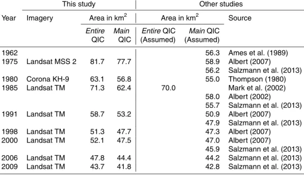
The CV and the QIC are located in the central Andes in southeastern Peru (Fig. 1), specifically, in the southern portion of the eastern branch (Cordillera Oriental) of the Peruvian Andes (Hastenrath, 1998). We have used the general geographic definition 20

of the CV as provided by Morales Arnao (1998), and in this study we refer to this as the entire CV study area. The CV mountain range is among the highest in Peru, with the highest peak (Nevado Ausangate) at 6384 m a.s.l. (above sea level), and glaciers terminating around 4700–5000 m a.s.l. (Salzmann et al., 2013). Climatically, the CV region experiences one thermal season with nearly constant temperatures and high 25

(6)

TCD

7, 573–634, 2013

from 1975 to 2012

Title Page

Tables Figures

◭ ◮

Back Close

Full Screen / Esc

Discussion

P

a

per

|

Dis

cussion

P

a

per

|

Discussion

P

a

per

|

Discussio

n

P

a

per

|

to September/October) (Vuille et al., 2008b; Rabatel et al., 2013) with a similar sea-sonality of humidity (Rabatel et al., 2012). Most of the precipitation falls during the wet season, the glacier accumulation season. Ablation, however, while more dominant during the April to November dry season, also occurs year round due to the high solar radiation and constant temperatures at the high altitudes of the CV (Vuille et al., 2008a). 5

Additionally, on interannual timescales, the El Ni ño Southern Oscillation (ENSO) is re-ported to have a significant influence on the climate in this region (Vuille et al., 2008a; Albert, 2007; Rabatel et al., 2013; Salzmann et al., 2013), with La Ni ña years tend-ing to be cooler and wetter, and El Ni ño years tendtend-ing to be warmer and dryer (Vuille

et al., 2008a; Rabatel et al., 2013). How this affects glacier mass balance in the CV,

10

however, has yet to be systematically investigated. The regions in southeastern Peru

are characterized by a very steep precipitation gradient and orographic rainfall effect

created by the eastern Andean slopes (Bookhagen and Strecker, 2008) (Fig. 1c),

rang-ing from>3 m yr−1annual rainfall at the mountain front to<0.25 m yr−1rainfall on the

high-elevation, arid Altiplano. 15

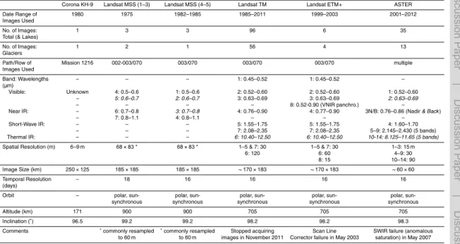
3 Data sources

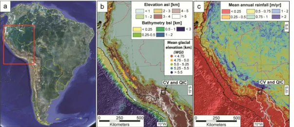
To create our glacial and lake area inventory, we used a variety of optical and multi-spectral satellite imagery, including Landsat Multi-Spectral Scanner (MSS), Thematic

Mapper (TM) and Enhanced Thematic Mapper Plus (ETM+), Advanced Spaceborne

Thermal Emission and Reflection Radiometer (ASTER), and declassified Corona KH-9 20

imagery. The characteristics of each of these sensors can be found in Table 1, and an example of each of these images can be seen in Fig. 2.

We have obtained a total of 108 usable Landsat images (6 MSS from 1975–1985, 96

TM from 1985–2011, 6 ETM+from 1999-2003), 35 ASTER images (from 2001–2012),

and 1 KH-9 Corona image from 1980, for a total of 144 images dating from 1975 to 25

2012. All 144 images were used to create a lake area time series, although not every

(7)

TCD

7, 573–634, 2013

from 1975 to 2012

Title Page

Tables Figures

◭ ◮

Back Close

Full Screen / Esc

Discussion

P

a

per

|

Dis

cussion

P

a

per

|

Discussion

P

a

per

|

Discussio

n

P

a

per

|

a specific lake. 77 images (63 Landsat, 1 Corona, and 13 ASTER) were used to create the glacial area time series, with images containing a range of 1 to all (10 identified)

of the glacierized regions located within this Landsat TM/ETM+ scene (Fig. 2a), as

similarly to the lakes, not all images could be used for all glacierized regions due to classification problems. Specifically for this area, obstruction by cloud cover limits the 5

images that can be used to the dry season (Rabatel et al., 2012), during which con-vective storms are more rare. However, storms producing transient snow cover do still occur during the dry season, and this local/regional snow can prevent obtaining accu-rate glacierized region outlines. For this reason, we have only used images, or parts of images (as this snow is often localized), where no transient snow cover exists. For more 10

information regarding the images used, please refer to Table SM A1 in the Supplement. In addition to the multi-spectral satellite imagery, this study used the 2000 Shut-tle Radar Topography Mission (SRTM) Digital Elevation Model (DEM) (version 4).

Ac-quired within 11 days during February 2000, this mission provided near-global (∼60◦N

to 56◦S latitude) digital elevation data at a horizontal resolution of∼90 m (Farr et al.,

15

2007). Linear vertical absolute and relative height errors are less than 16 m and 10 m respectively, decreasing to 6.2 m and 5.5 m respectively for South America (Farr et al., 2007). For this study, these data were resampled to 15 m using bilinear interpolation. We also worked with the ASTER Global Digital Elevation Model (GDEM V1 and V2), a DEM created from ASTER imagery taken over the course of a decade. Since glacial el-20

evations are likely to change over 10-yr time periods, inconsistencies over glaciers and

shadowing effects from topography and clouds prevented us from using the ASTER

GDEM.

4 Methodology

The creation of lake, glacier, and snowline outlines are multi-step processes with some 25

(8)

TCD

7, 573–634, 2013

from 1975 to 2012

Title Page

Tables Figures

◭ ◮

Back Close

Full Screen / Esc

Discussion

P

a

per

|

Dis

cussion

P

a

per

|

Discussion

P

a

per

|

Discussio

n

P

a

per

|

pan-sharpening (base-image only), resampling if necessary (ASTER Short Wave Infra-Red (SWIR) 30 m to 15 m), conversion to reflectance (all ASTER images, and Land-sat images used for snowline analysis, converted to reflectance using standard

tech-niques), and aligning to the base image (all images). For this study, a Landsat ETM+

image from 24 June 2000 (path 003, row 070, Fig. 2a) was chosen as the base image 5

as this image covered the entire study region with no clouds and good gain control, im-portant factors when aligning images or calibrating images for reflectance. We

specifi-cally used a Landsat ETM+image for this, as Masek et al. (2001) report that Landsat

ETM+ has decreased noise levels and increased radiometric precision compared to

Landsat TM 5. 10

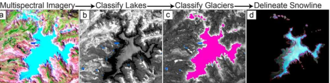
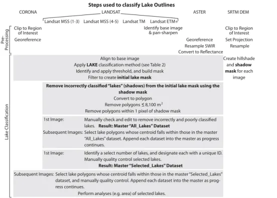
The general process used to classify the images is outlined in Fig. 3. Upon com-pletion of pre-processing, the first step was to classify the lakes in each image, i.e. to create a lake mask (Sect. 4.1). This was done using simple band ratios and filter-ing, removal of shadows using a hillshade mask for each image, followed by manual editing (Huggel et al., 2002). Glaciers were classified similarly using simple ratios (Svo-15

boda and Paul, 2009) (Sect. 4.2). Subsequently, the previously created lake mask was applied to the ratio image, to remove incorrectly classified lakes. Manual editing and validation was a required final step. In determining the snowline for a particular glacier (Sect. 4.3), a calibrated reflectance image was first clipped to the glacier extent using this glacier mask. After selecting snow and ice regions, we then performed a Multiple 20

Endmember Spectral Mixture Analysis (MESMA) (Klein and Isacks, 1999; Roberts et al., 1998). To create files usable in further analysis, all rasters are converted to poly-gons.

4.1 Lake area mapping

Our primary purpose of lake extraction is to correct and refine glacial mapping by out-25

(9)

TCD

7, 573–634, 2013

from 1975 to 2012

Title Page

Tables Figures

◭ ◮

Back Close

Full Screen / Esc

Discussion

P

a

per

|

Dis

cussion

P

a

per

|

Discussion

P

a

per

|

Discussio

n

P

a

per

|

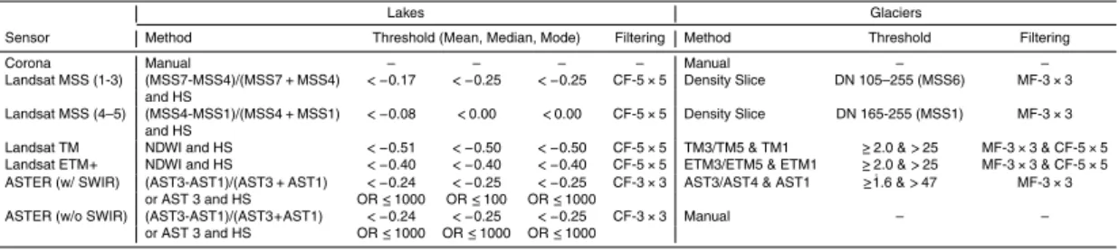
Lakes in glacial regions often have a variety of biological and physical components (e.g., pollen and sediment) influencing their color, and the employed methodology

must be able to distinguish varying colors. For the Landsat TM/ETM+ imagery we

pursued the methodology outlined in Huggel et al. (2002) using the Normalized

Dif-ference Water Index (NDWI: Landsat bands (TM4-TM1)/(TM4₊TM1)) followed by a

5

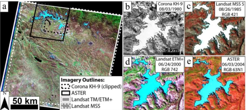
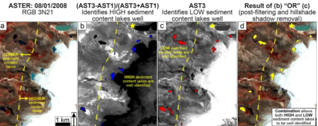
hillshade mask. This NDWI performed well to classify lakes with a range of suspended sediment concentrations. ASTER images were processed in the same fashion as the

Landsat TM/ETM₊images, however, they proved more complicated due to their lack

of a “blue” band (0.45–0.52 µm, equating to Landsat B1, see Table 1). Previous stud-ies have used the green band as an alternative, resulting in an approximation of the 10

NDWI algorithm using (AST3-AST1)/(AST3₊AST1) (Bolch et al., 2008). While this

in-dex performed fairly well to identify lakes with higher concentrations of suspended sed-iment (typically found in close proximity to glaciers), it was unable to capture lakes with lower concentrations of suspended sediment as successfully. To classify lower sedi-ment content lakes, a threshold in ASTER B3 proved successful, but alternatively was 15

not always successful at identifying the higher sediment content lakes. A combination of both the ASTER NDWI-approximation algorithm and ASTER B3 provided the most suitable method to identify lakes with the greatest range of suspended sediment con-centrations. Unfortunately, this combination method could not identify all lakes through-out the study region. Figure 5 through-outlines the method used to classify lakes in the ASTER 20

imagery, illustrating where each method works and does not work.

After initial classification and filtering, shadows were removed using a hillshade mask and some manual editing, resulting in a master lake file containing only lakes for each image. We then selected, and manually quality controlled, fifty lakes that were typically well classified (large and small, high and low sediment concentrations, near and far 25

(10)

TCD

7, 573–634, 2013

from 1975 to 2012

Title Page

Tables Figures

◭ ◮

Back Close

Full Screen / Esc

Discussion

P

a

per

|

Dis

cussion

P

a

per

|

Discussion

P

a

per

|

Discussio

n

P

a

per

|

4.2 Glacier area mapping

Debate continues on the best method to be used for delineating glacial outlines, with

different studies suggesting different methods as superior (Paul and K ¨a ¨ab, 2005;

Raco-viteanu et al., 2009, 2008b). The consensus that seems to have been reached is that it depends on the test site in question. Manual delineation is very time consuming 5

and can be highly subjective. Band ratios and thresholds provide the best

compro-mise between processing time and accuracy, with an estimated accuracy difference

of<3 % between the three most often used techniques: Landsat bands 3/5, 4/5, and

the Normalized Difference Snow Index (Albert, 2002). In our study, we followed the

methodology outlined in Svoboda and Paul (2009) using Landsat (TM/ETM₊) bands

10

3/5 and ASTER bands 3/4, followed by a threshold in Landsat and ASTER bands 1 to include snow and ice in cast shadow. Their MSS classification scheme worked poorly for our images, and so we classified the glacierized areas in the MSS images using a single-band thresholding process. Unfortunately, this method provides only a minimum areal extent, as snow and ice in shadow are completely ignored. The glaciers in the 15

Corona and ASTER images lacking SWIR bands were manually delineated. While not all images are suitable for glacier classification (local/regional snow cover or clouds obscuring outlines), our study classified as many images as possible to gain as much information as possible on how the glacierized regions behave on an annual as well as a decadal time scale. The general steps involved in the glacier classification of each 20

group of imagery are summarized in Fig. 6, with the methods and thresholds used for each set of imagery summarized in Table 2.

Upon creation of the initial glacier mask, post-classification and filtering, the previ-ously created lake masks for each image were applied to each glacier mask to remove

incorrectly classified lake pixels. Subsequently, polygons with areas≤10 000 m2

(cor-25

responding to 11, 44, 2, and 177 pixels for Landsat TM/ETM+, ASTER, Landsat MSS

(11)

TCD

7, 573–634, 2013

from 1975 to 2012

Title Page

Tables Figures

◭ ◮

Back Close

Full Screen / Esc

Discussion

P

a

per

|

Dis

cussion

P

a

per

|

Discussion

P

a

per

|

Discussio

n

P

a

per

|

1975) we identified and assigned a unique ID to discrete glacierized areas (closed ice masses or polygons that are nearby or that appeared to be part of that same glaciated

mass) throughout the Landsat TM/ETM+ scene extent encompassing the entire CV

area. Working in chronological order from 1975 to 2011, these IDs were assigned to polygons falling within those of their earliest outline (the assumed largest glacierized 5

area). For each image, we have only included those glacierized areas if the entire outlines are completely unobstructed by clouds or obscured by local snow. Similar to Salzmann et al. (2013), we have not separately mapped debris covered glaciers as these areas are expected to be minimal in this region. A more detailed description of the glacier classification process can be found in the Supplement (Appendix B2). 10

4.3 Snowline mapping

On some images from the mid-late ablation season, the snowlines are clearly visible.

Classifying these snowlines, however, proved difficult. Many of the suggested

meth-ods proved unsatisfactory for this region, for example, Landsat TM bands 4/5 (Hall et al., 1987), Landsat TM bands 3/4 and 3/5, and maximum likelihood classification of 15

principal components (Bronge and Bronge, 1999), maximum likelihood classification of principal components on ASTER imagery (Mathieu et al., 2009), and a two-step

un-supervised classification process based on Landsat ETM₊bands and algorithms and

snow/ice texture (Yu et al., 2012). While Rabatel et al. (2005) manually delineated the ELA on three glaciers in the French Alps, we pursued the methodology suggested by 20

Klein and Isacks (1999) for the Zongo glacier in Bolivia and the QIC: spectral mixture analysis (e.g., Painter et al. 1998). Spectral unmixing has also been successfully used by Chan et al. (2009) in delineating the snowline and the area accumulation ratio for the Morteratsch glacier in Switzerland. In our study, we focus on the QIC, initially creating a spectral library of snow and ice endmembers per usable image. A small selection of 25

(12)

TCD

7, 573–634, 2013

from 1975 to 2012

Title Page

Tables Figures

◭ ◮

Back Close

Full Screen / Esc

Discussion

P

a

per

|

Dis

cussion

P

a

per

|

Discussion

P

a

per

|

Discussio

n

P

a

per

|

and ice, allowing for classification of regions that are dominantly snow (accumulation zone) or dominantly ice (ablation zone). Performing this methodology (Fig. 7) on mul-tiple images produced a time series for the snowline of the QIC. As with the lake and glacier classifications, more information on the snowline classification can be found in Appendix B3 of the Supplement.

5

All usable images (conditions were satisfactory in 17 images) were converted to reflectance and calibrated to the reflectance of the base image. After selecting repre-sentative endmember regions in each image, we used techniques described in Roberts et al. (2007) to create spectral libraries for each, and subsequently to identify optimum spectra for these endmembers, specifically using the metrics CoB (Count Based End-10

member Selection), EAR (Endmember Average RMSE), and MASA (Minimum Average Spectral Angle). This resulted in 37 ice spectra and 8 snow spectra for our Landsat

im-agery. These optimized spectra, with their strong spectral differences between snow

and ice that make this method robust (Fig. 8), were then run on each snowline image using MESMA.

15

Post-MESMA processing includes applying a threshold to the snow endmember classification, where regions with snow (rather than ice) were determined to be in pixels

>50 % snow (this threshold was determined by visual examination, and corroborates

what is estimated in another study; Chan et al., 2009). After filtering, the outline was converted to points and SRTM DEM values at those points extracted, to determine the 20

elevation of the snowline.

5 Results

We first present our glacial results by focusing on the two largest glacierized regions in our study area: the Quelccaya Ice Cap (Glacial ID: 1), and the largest continuous (main) glacierized region in the Cordillera Vilcanota (Glacial ID: 2), in addition to results for the 25

(13)

TCD

7, 573–634, 2013

from 1975 to 2012

Title Page

Tables Figures

◭ ◮

Back Close

Full Screen / Esc

Discussion

P

a

per

|

Dis

cussion

P

a

per

|

Discussion

P

a

per

|

Discussio

n

P

a

per

|

which we present our time series of the QIC snowline. Additional glacial and lake area results can be found in the Supplement (Appendix C1 and C2, respectively).

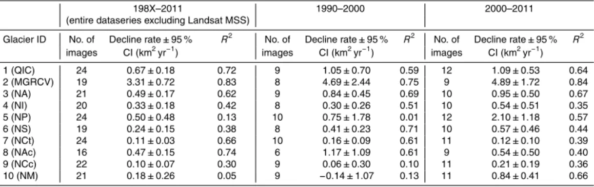
5.1 Glacier area changes

5.1.1 Quelccaya Ice Cap (QIC)

Our results indicate that the QIC has decreased in area by 42 % over the time period 5

1975–2011 (Fig. 10). Because the Landsat MSS data have lower spatial resolution and were classified using single band density slicing, we exclude the MSS data from our regression analysis (all regressions are unweighted). Between 1980 and 2011, an area

of 15.5 km2of the QIC was lost (an area that represents 25 % of the 1980 QIC extent).

Using only the minimum area measurements for each year, this represents an aver-10

age decline rate of 0.67±0.18 km2yr−1(all uncertainties are 95 % confidence intervals

unless otherwise noted). However, this decline has not been constant; our time series shows that there have been some important interannual variations in glacierized area – significant increases in glacierized area were observed during the early 2000s and more recently in 2011. Decline rates for the QIC increase in the 1990s and 2000s to 15

1.05±0.70 km2yr−1and 1.09±0.53 km2yr−1, respectively (Table 3).

Glacial-area uncertainties (error bars) are calculated using perimeter and grid-cell size of imagery, following:

Error (95 % confidence interval)=(P/(G·0.6872/2))·G2 (1)

whereP=perimeter andG=grid-cell size (spatial resolution).

20

5.1.2 Cordillera Vilcanota (CV)

(14)

TCD

7, 573–634, 2013

from 1975 to 2012

Title Page

Tables Figures

◭ ◮

Back Close

Full Screen / Esc

Discussion

P

a

per

|

Dis

cussion

P

a

per

|

Discussion

P

a

per

|

Discussio

n

P

a

per

|

mountain range (Glacial ID: 2, Fig. 11) has seen a reduction in area of 109.7 km2

be-tween 1985 and 2011 (40 % of its 1985 area). Additionally, this glacierized region has an approximately five-times higher decline rate from 1985–2010 than that of the QIC,

declining an average of 3.32±0.74 km2yr−1(using minimum areas). As with the QIC,

this decline has not been constant and glacierized area temporally increased during the 5

late 1990s and early 2000s, before continuing its overall decline (Fig. 11). The 1990s and 2000s have high decline rates for the main glacierized region of the CV (MGRCV),

with decline rates of 4.69±2.44 km2yr−1(1990–2000) and 4.89±1.72 km2yr−1(2000–

2011). For this particular glacierized region, Landsat MSS images seemed to underes-timate the extent of the glacierized area, likely due to increased shadow regions in the 10

images used.

In the 22 yr between 1988 and 2010 (using only Landsat TM/ETM₊ imagery), all

glacierized regions throughout the entire Cordillera Vilcanota (Glacial IDs 1–7, 9–10,

but not ID 8) declined by a total of 118.7 km2 (32 % of 1988 extents). Including the

MSS value from 1985 (likely an underestimate), this total decline increases to 35 % 15

between 1985 and 2010 (Fig. 12). In Fig. 12 we also include data reported for the CV by Salzmann et al. (2013) to (1) illustrate how our measurements align with respect to their measurements (our measurements correspond well, within the error bars, of their 1996 and 2006 measurements, however, our 1985 measurement is somewhat below theirs, although we note that ours is likely an underestimate), and (2) to illustrate how 20

the use of multiple images and measurements, as used in this study, provides much more information on glacial decline and advance over this time period. For example, note the steep decrease in glacial area throughout the entire CV during 1998, which would be uncaptured were fewer measurements obtained. The table insets in Fig. 12 compare our decline rates to those of Salzmann et al. (2013), using our minimum 25

values during the relevant time periods, rather than just 2 data points for each. For the 1962 value, we also use the measurement from Ames et al. (1989).

To summarize, for the time period of 1988 through 2010 (TM/ETM+only), the decline

(15)

TCD

7, 573–634, 2013

from 1975 to 2012

Title Page

Tables Figures

◭ ◮

Back Close

Full Screen / Esc

Discussion

P

a

per

|

Dis

cussion

P

a

per

|

Discussion

P

a

per

|

Discussio

n

P

a

per

|

using MSS from 1985). This decline rate increased during the 1990s (1990–2000) to a

decline rate of 12.51±11.83 km2yr−1(n=6,r2=0.6), and then decreased slightly

dur-ing the first decade of the 21st century (2000–2011), to a decline rate of 9.04±2.51 km2

yr−1(n=8,r2=0.9). However, these decline rates are for the entire CV area, which are

dominated by the largest glacierized region (Glacial ID: 2). Each of the glacierized re-5

gions within the CV (IDs 1–7, 9–10), have declined at different rates (Table 3). For

the individual glacierized regions we report mostly increasing decline rates during the 2000s (2000–2011) over those of the 1990s (1990–2000) (Fig. 13). We also note that on average, smaller glaciers have higher decline rates than larger glaciers (Fig. 13, Table 4).

10

5.2 Lake area changes

Our lake area time series (1975–2012) includes 50 lakes (Fig. 9). Here, we present the results of three characteristic proglacial lakes: an existing large proglacial lake (Laguna Sibinacocha (Lake ID: 2), Fig. 14), and two recently formed (1985) proglacial lakes (Lake ID: 8, Fig. 15, downstream of Nevado Ausangate (Glacial ID: 3), and Lake ID: 33, 15

Fig. 16, a proglacial lake in front of Qori Kalis glacier, QIC (Glacial ID: 1)). Additionally, Fig. 17 summarizes how eight lakes surrounding the QIC have been changing with respect to the QIC’s glacial area. We present additional results for lake area changes in the Supplement (Appendix C2).

Unlike glacierized regions, proglacial lake areas vary more widely both temporally 20

and spatially, reflecting a variety of di_fferent melting processes, including GLOFs.

La-guna Sibinacocha (Lake ID: 2, Fig. 9, Fig. 14) is a large (15-km long) lake extending south from the tongue of one of the southern glaciers in the MGRCV (Glacial ID: 2). This particular lake is used for hydropower generation (Salzmann et al., 2013). Already

the second largest lake in this region (the first being Laguna Langui, at∼54.5 km2),

La-25

guna Sibinacocha increased in area by 12 % (from 25.3 km2to 28.2 km2) between 1982

(16)

TCD

7, 573–634, 2013

from 1975 to 2012

Title Page

Tables Figures

◭ ◮

Back Close

Full Screen / Esc

Discussion

P

a

per

|

Dis

cussion

P

a

per

|

Discussion

P

a

per

|

Discussio

n

P

a

per

|

which the lake area was relatively stable, but after which the lake area has fluctuated more widely.

In contrast to Laguna Sibinacocha (Lake ID: 2), the proglacial Lake ID 8 beneath the Nevado Ausangate region did not exist before 1985 (Figs. 9 and 15). Since then, how-ever, this lake has rapidly developed, beginning during the late 1990s but particularly 5

during the early 2000s, growing at an average rate of 12,605±1030 m2yr−1. Since the

beginning of 2010, however, it appears as though the lake area has begun to decline. Similar results can be seen for Lake ID 33 (a proglacial lake in front of Qori Kalis glacier in the QIC) (Fig. 16). Growth of this lake has been previously documented (Brecher and Thompson, 1993; Thompson et al., 2006) and reflects the retreat of 10

Qori Kalis glacier (Fig. 21). Both Thompson et al.’s (2006) 1991–2005 retreat rate of

∼60 m yr−1and this study’s retreat rate of∼67 m yr−1correspond with the time period

during which this lake experienced the majority of its growth. The period 2000–2005 showed even greater lake growth than during the previous 9 yr since 1991. This reflects our findings in this study of the higher glacial decline rates during the 2000s than dur-15

ing the 1990s, and the related growth of this proglacial lake in correspondence to this. In general, we note that areas of proglacial lakes have typically been fairly constant

for∼15–20 yr preceeding 2002. Since 2002, however, proglacial lake areas began to

rapidly increase. For the 8 lakes surrounding the QIC (Fig. 17) we note that post-2002, after rapid lake area increases and decreases over short time intervals, the lake areas 20

have been highly fluctuating, despite fairly constant decline in the QIC glacial area.

5.3 Snowlines

Remote sensing studies in recent years have used the transient snowline at the end of the ablation period, or end of summer snowline (EOSS), as a proxy for the equilibrium line altitude (ELA) of a given year (Klein and Isacks, 1999; Østrem, 1975; Mathieu et 25

(17)

TCD

7, 573–634, 2013

from 1975 to 2012

Title Page

Tables Figures

◭ ◮

Back Close

Full Screen / Esc

Discussion

P

a

per

|

Dis

cussion

P

a

per

|

Discussion

P

a

per

|

Discussio

n

P

a

per

|

that the highest altitude reached by the snowline over the course of the entire ablation season (not just the EOSS) may provide an estimate of the ELA for that year (although it is likely an underestimation). In this study, we used spectral unmixing methods to delineate transient snowline elevations for the QIC from 1988 to 2010 using Landsat

TM and ETM₊imagery (Fig. 18). Conditions were suitable for this purpose in only 17

5

images. We observed large inter-annual fluctuations, with high median snowline ele-vations in the late 1990s. Figure 18 reports our results alongside those from previous studies, but only minimal snowline measurements exist in the literature, whether de-termined in situ or using remote sensing methods. For the QIC, the lowest altitude that the snowline reached using results from this study was in 1989 (22 September), 10

with a median altitude of 5287 m a.s.l. In 1998 (15 September) it reached its maximum of 5582 m a.s.l., almost 300 m higher. In 2010 (16 September), our most recent

mea-surement, the snowline had descended to 5432 m a.s.l.,∼150 m above its minimum

altitude in 1989. Unfortunately, because no field measurements of the ELA for the QIC exist during our period of study, we are unable to validate our results. However, based 15

on the relationship between snowline altitude (SLA) and ELA as reported in Rabatel et al. (2012), our measurements are likely to represent minimum estimates of the ELA for the given years (as the SLA on satellite images tends to be an underestimate of the ELA; Rabatel et al., 2012). In Fig. 18 we have chosen only to indicate positive errors in response to the fact that these SLAs are minimum ELA estimates. The trend still 20

indicates that the elevation of the transient snowline of the QIC is increasing, at an

average rate of 2.8±4.5 m yr−1 between 1988 and 2010 (Fig. 18). Our errors appear

to be large, but they reflect the SLA surrounding the entire QIC and are surprisingly robust.

6 Discussion

25

(18)

TCD

7, 573–634, 2013

from 1975 to 2012

Title Page

Tables Figures

◭ ◮

Back Close

Full Screen / Esc

Discussion

P

a

per

|

Dis

cussion

P

a

per

|

Discussion

P

a

per

|

Discussio

n

P

a

per

|

caveats when comparing glacial and lake area changes between different studies and

methodologies.

6.1 Glacier area changes

6.1.1 Quelccaya Ice Cap (QIC)

In the previous section (Sect. 5.1.1), we illustrate the dramatic decline of the QIC (25 % 5

between 1980 and 2011). This result agrees with that of Salzmann et al. (2013), who report a reduction in glacial area of 23 % between 1985 and 2009. In general, our satellite-derived glacial-area measurements correlate well with previous satellite esti-mates where boundary conditions were similar. However, comparing methodologies and glacial areas between studies is not always straight forward. Specifically, in the 10

case of the QIC, it is evident that di_fferent studies seem to use di_ffering outlines for the

extent of the QIC (Fig. 19, Table 5). We use the termentireQIC (Fig. 19a) to refer to all

snow-covered regions identified in the earliest image (28 October 1975) and the term

main QIC (Fig. 19b) to identify the largest, continuous ice mass. Additionally, some

studies (e.g., Hastenrath, 1998; Mark et al., 2002; Thompson, 1980) provide an area 15

measurement merely informatively and tend to neglect to provide the specific dates of the imagery (or methods) with which they determined the area. Other studies (e.g., Al-bert, 2002, 2007; Salzmann et al., 2013) have specifically investigated and reported the area and dates (at least, mostly) as part of their study, but provide less specific information on the extent of the QIC which was used. Comparing our results to those 20

of other studies (Table 5), it appears that the majority of studies primarily use just the main QIC to determine the area, based on the fact that these results are closest to ours of the main QIC alone. This seems to be the case for Albert (2007), and while Salzmann et al. (2013) appear to use an extent that includes some outlying areas be-yond the main QIC alone, they appear to not include the NW part of the ice cap, a 25

(19)

TCD

7, 573–634, 2013

from 1975 to 2012

Title Page

Tables Figures

◭ ◮

Back Close

Full Screen / Esc

Discussion

P

a

per

|

Dis

cussion

P

a

per

|

Discussion

P

a

per

|

Discussio

n

P

a

per

|

used, and the long extent of the time series in this study and therefore suggest that our data are robust.

Additional discrepancies between glacial-area measurements are caused by the time of year the satellite image was taken. The more images in a given year, the more visible this trend is. The data density of several reliable satellite images per year for 5

some years allows us to see the (inter-) annual fluctuations in glacierized area (Figs. 10, 11, and 20). We note increasing areas over the wet winter accumulation period and then declining areas throughout the course of the dry summer ablation period (Fig. 20 zooms into the 2005–2012 time period of Fig. 10). For example, in 2009, the area of theentireQIC (Figs. 10 and 20) varied by 5 km2 (10 %), from 48.7 km2 on 8 May, the 10

earliest usable image after the accumulation period, to 43.7 km2on 31 October, at the

end of the ablation period. Six images over the course of 2009 document this steady decline. Although only 3 images exist for 2011, that year underwent an even more

drastic decline of 11.1 km2(19 %), from an area of 58.7 km2on May 14 to 47.6 km2on

3 September. This illustrates how area measurements can vary even up to 19 % in a 15

given year, and emphasizes how important it is to give the date of measurement when reporting area results for glacierized regions.

Our satellite-based measurements correspond fairly well with those from other stud-ies (Table 5), with the exception of 1975. Visual examination indicates that the MSS density slice classification delineates the QIC well for this image. We do not know the 20

date of the image used for Salzmann et al.’s (2013) study, and can only suggest that

the date of the imagery used, and the extent of the area termed the QIC are different

between our two studies. Kaser and Georges (1997) report that there was a period of glacial advance in the mid-1970s, and perhaps our 1975 area measurement reflects this.

25

(20)

TCD

7, 573–634, 2013

from 1975 to 2012

Title Page

Tables Figures

◭ ◮

Back Close

Full Screen / Esc

Discussion

P

a

per

|

Dis

cussion

P

a

per

|

Discussion

P

a

per

|

Discussio

n

P

a

per

|

glacial extents to field measurements for the Qori Kalis glacier (Thompson et al., 2006). While there are some discrepancies that are likely a result of measurements taken at

different times of the year, the overall patterns match. Although our study does not have

measurements for Qori Kalis dating back to 1963, the trends in the data are similar.

Thompson et al. (2006) report a frontal retreat rate of∼6 m yr−1 for Qori Kalis during

5

the 15 yr period from 1963–1978, and a∼10 fold increase during the next 14 yr, from

1991–2005 (a retreat rate of ∼60 m yr−1). Our satellite-based study supports these

findings, with a retreat rate of∼9–10 m yr−1during the shorter time period 1980–1991,

but a similar retreat rate of∼67 m yr−1during the subsequent 14 yr period from 1991–

2005. This retreat corresponds to the development of the proglacial lake (Lake ID: 33) 10

shown in Fig. 16.

6.1.2 Cordillera Vilcanota (CV)

As with the QIC, different studies use differing extents of the CV region. As previously

mentioned in Sect. 2, our study uses the geographic definition as provided by Morales Arnao (1998) and incorporates this study’s Glacial IDs 1–7 and 9–10. Glacial ID 8 is 15

located beyond the CV and is not included in measurements where we discuss the

entireCV. For their definition of the CV extent, between 1985 and 2006, Salzmann et al. (2013) report a 33 % loss in glacierized area. Over a similar time frame, from 1988 to 2010, our study reports a 32 % loss in area. Our definition of the extent of the CV

region may incorporate slightly differing glacierized regions, however, the trends are

20

comparable.

For their definition of the CV, Salzmann et al. (2013) report high decline rates (9.1 km2

yr−1) from 1985–1996, with slower decline rates (4.7 km2yr−1) from 1996–2006 and

ac-tually a slight growth rate (0.2 km2yr−1) for the earlier period from 1962–1985, based

on two images per time period (Fig. 12). Based on two images per time period, our 25

data report a 3.4 km2yr−1decline rate for the period 1985–1996 (a CV area of 390 km2

on 26 August 1985 (Landsat MSS) and 353 km2on 21 June 1996 (Landsat TM)), and a

(21)

TCD

7, 573–634, 2013

from 1975 to 2012

Title Page

Tables Figures

◭ ◮

Back Close

Full Screen / Esc

Discussion

P

a

per

|

Dis

cussion

P

a

per

|

Discussion

P

a

per

|

Discussio

n

P

a

per

|

on 19 July 2006 (Landsat TM)), although this rate is slightly lower (5.3 km2yr−1) if a date

a month earlier is used (300 km2on 17 June 2006). However, our data allows us to

cal-culate decline rates from 1996–2006 using 7 images (using minimum areas for each

year) for each glacial ID, which results in an average decline rate of 6.09±9.61 km2yr−1

(r2=0.2). Again, we emphasize the necessity to include date measurements when

re-5

porting area measurements, as Fig. 20 shows that area measurements can even vary by up to 19 % within a year.

Because results based on single images alone can be biased, we have chosen to calculate our decline rates using as many images in the specific time periods as pos-sible. To obtain as accurate an estimate of the decline as possible, we have limited the 10

images used to calculate these decline rates to those that represent the minimum area measured for that year. Unfortunately, multiple images do not exist for all glacial IDs for all years, and in these cases the minimum area measurement is actually the only mea-surement. As a result, decline rates are also minimum estimates. Additionally, we also omit the Landsat MSS images because of their coarser spatial resolution and fewer 15

channels, and have therefore calculated decline rates only with the Landsat TM/ETM+

imagery, since consistency is maintained in methodology throughout this dataset from

1985 to 2011. We have calculated decline rates for three different time periods (Fig. 13,

and Table 3 (not normalized against area) and Table 4 (normalized against median area of each glacial ID’s earliest Landsat TM outline). Our study finds that area-normalized 20

decline rates for the majority of glacierized regions investigated (8 of 10) are highest during the period 2000–2011. The 1990s still showed high decline rates with 7 out of 10 glacierized regions reporting higher decline rates during the 1990s than over the course of the entire time period (Fig. 13 and Table 3). However, our results do support other studies which report higher decline rates during the 1990s when we calculate decline 25

rates for the entire CV as a whole (a 1990–2000 decline rate of 12.51±11.83 km2yr−1

(r2=0.6), and a 2000–2011 decline rate of 9.04±2.51 km2yr−1 (r2=0.9)). These

de-cline rate patterns are different to those for individual glacierized areas alone because

(22)

TCD

7, 573–634, 2013

from 1975 to 2012

Title Page

Tables Figures

◭ ◮

Back Close

Full Screen / Esc

Discussion

P

a

per

|

Dis

cussion

P

a

per

|

Discussion

P

a

per

|

Discussio

n

P

a

per

|

to size, the majority of the smallest glacierized regions (<∼12–20 km2) show the

over-all highest area-normalized decline rates, particularly from 2000–2011 (Fig. 13 and Table 4). Our study presents decline rates deduced from a minimum of 16, and a max-imum of 24, images over the time period 198X to 2011 for each glacierized region, which show a strong increase in areal decline rates. (If we were to use all images 5

rather than only the minimum area images for each year, the number of images would increase to 31 and 63, respectively.) This increase in areal decline rates is an impor-tant finding, as other studies suggest that decline rates have been decreasing since the mid-1980s to mid-1990s, although they are likely using the region as a whole to calculate their decline rates. Our study suggests that decline rates are not decreasing, 10

but instead are increasing for most glacierized areas in the CV region compared to the 1980s and 1990s.

We investigated the areal glacial retreat behavior with respect to elevation by analyz-ing the median elevation of a glacier through time. We observed that all median glacial

elevations rose through time, but their rates differed with respect to elevation (Fig. 22).

15

Glacierized areas with lower median elevations are retreating faster than glacierized

areas at higher elevations (Fig. 22). For the 4 largest glacierized areas (>20 km2) in

the CV and just beyond, the median elevation gain ranged from 1.77±0.43 m yr−1 to

2.91±0.51 m yr−1. Median glacial elevations around 5200 m a.s.l. have been retreating

to higher elevations at a rate of about 1 m yr−1 faster than glaciers located only 200 m

20

higher at 5400 m a.s.l. These results reflect those found in Rabatel et al. (2013), specif-ically, that glaciers lower than 5400 m a.s.l. have been losing mass at a greater rate

(1.2 m w.e. yr−1 (meters of water equivalent yr−1)) than those glaciers located higher

than 5400 m a.s.l. (0.6 m w.e. yr−1). The majority of glaciers in this region terminate

around 4700–5000 m a.s.l. (Salzmann et al., 2013) and will thus retreat more rapidly 25

(23)

TCD

7, 573–634, 2013

from 1975 to 2012

Title Page

Tables Figures

◭ ◮

Back Close

Full Screen / Esc

Discussion

P

a

per

|

Dis

cussion

P

a

per

|

Discussion

P

a

per

|

Discussio

n

P

a

per

|

6.2 Lake area changes

No studies exist examining proglacial and glacier-fed lake area changes in the northern central Andes. This is the first regional study summarizing lake area changes derived from satellite imagery. The majority of lakes in this region that we tracked have been

small: 41 out of 50 (or 82 %) are less than 2 km2, and only 3/50 (or 6 %) are larger than

5

5 km2. Smaller lakes have larger errors associated with their area measurements, and

many of our identified lakes fluctuate widely. This is likely a result of unstable lake areas,

classification methodology, and the fact that many images required different thresholds

to visually outline the same lake area. These factors make interpreting a signal through

time difficult. However, some lakes show clear signals, particularly the proglacial lakes,

10

of which we have shown the results specifically for three in this study (Figs. 14,15, and 16) in addition to those surrounding the QIC (Fig. 17). In this study we focus on the

lakes that are not readily affected by size limitations and classification thresholds.

We observed the rapid development of two proglacial lakes since 1985 that previ-ously did not exist (Figs. 15 and 16). The development of these lakes reflects glacial 15

retreat in this region, with the period 2000–2010 showing greater lake growth than dur-ing the previous 8 yr since 1992, or 15 yr since 1985. This agrees with our finddur-ings of higher glacial decline rates during the 2000s than during the 1990s.

Laguna Sibinacocha (Lake ID: 2, Figs. 9 and 14) illustrates the growth of a lake sit-uated just downstream of a glacial tongue, a lake growth of 12 % in the three decades 20

between 1982 and 2011. This lake appears to have seen the majority of its growth dur-ing the mid-late 1990s, which corresponds well with the significant decrease in glacial area during the strong positive El Ni ˜no Southern Oscillation (ENSO) event of 1998, which has been suggested to impact glacial behavior in this region (Vuille et al., 2008a; Albert, 2007; Rabatel et al., 2013; Salzmann et al., 2013). At least, the coincidence 25

(24)

TCD

7, 573–634, 2013

from 1975 to 2012

Title Page

Tables Figures

◭ ◮

Back Close

Full Screen / Esc

Discussion

P

a

per

|

Dis

cussion

P

a

per

|

Discussion

P

a

per

|

Discussio

n

P

a

per

|

much wetter. We therefore hypothesize that this lake level change is a combination of enhanced glacial and permafrost melting at high elevation, in addition to more rainfall and precipitation at lower elevation.

The timing of this lake area increase is similar to other lake-area observations (IDs 8 and 33, Figs. 15 and 16, respectively), whose lake areas also began rapidly increasing 5

during the late 1990s. These lakes, however, increased more significantly during the early 2000s. In order to investigate the relationship between glacial decline and lake area increase in more depth, we have generated time series emphasizing the area changes (slopes) for eight proglacial lakes surrounding the QIC (Fig. 17, locations of lakes in Fig. 24). In 2001, glacial area rapidly increased, but then rapidly melted 10

during the subsequent year (2002). This rapid increase in meltwater caused all lakes surrounding the QIC to simultaneously increase, indicating how connected this rela-tionship between glacial melt and proglacial lake growth is.

In order to put our analysis into an expanded spatial context, we show the lake-area trend for all 50 identified lakes (Fig. 23). Using the SRTM DEM, we delineated the 15

watersheds for each of the lakes, and identified whether they were connected to glacial regions or not. The most recent lake area was normalized against the earliest lake area (using Landsat TM images only): values greater than 1 indicate growing regions, values less than 1 are declining.

The majority of declining lakes can be found in watersheds with no connection to 20

glacial meltwaters. Specifically, between the mid-late 1980s and 2011, 84.1 % of lakes not connected to glacial meltwaters have declined. In contrast, 61.3 % of lakes con-nected to glacial meltwaters have increased in area. This suggests again that lakes within glacial watersheds are benefiting from the increased glacial melting that has oc-curred over the time period of this study. In order to highlight the growth of proglacial 25

(25)

TCD

7, 573–634, 2013

from 1975 to 2012

Title Page

Tables Figures

◭ ◮

Back Close

Full Screen / Esc

Discussion

P

a

per

|

Dis

cussion

P

a

per

|

Discussion

P

a

per

|

Discussio

n

P

a

per

|

appear to be decreasing in area, although more data are needed to determine whether this is a pattern or not (Fig. 24).

Reporting specific values for our 50 identified lakes, between 1988 and 2010 (to align with the 1988–2010 glacial area measurements), lakes connected to glacial tersheds increased in area by 12.4 %. In contrast, lakes not connected to glacial wa-5

tersheds decreased in area by 1.9 % over the same period. As the trend in glacier-ized regions has been characterglacier-ized by significant glacial melting (32 % over the same time period), we hypothesize that lakes connected to glacial watersheds, and therefore glacial meltwaters, are increasing as a result of the decline in glacierized areas. In con-trast, lakes not connected to glacier watersheds are predominantly stable or declining 10

in area.

However, some drainage basins are characterized by cascading lakes and we ob-serve that some lakes closest to glaciers (i.e., the first or second lakes downstream of a glacier) are growing, whereas lakes further downstream may show an areally stable, or even declining, signal. For example, the north-westerly downstream section of the 15

MGRCV (Glacial ID: 2, Fig. 23).

To summarize, proglacial lakes (e.g., shown in Figs. 14, 15, and 16) are in good spa-tial and temporal agreement with glacial melting. Several of these lakes are dammed and constrained behind previous glacial moraines and they pose a dangerous natu-ral hazard to vulnerable downstream communities as the water builds behind these 20

moraines. Case studies on such natural hazards including GLOFs have been widely

documented in the Cordillera Blanca of Peru (Carey, 2005; Hubbard et al., 2005; Vil´ımek

et al., 2005; Hegglin and Huggel, 2008), north of this study area, but these hazards ex-ist in this region too.

6.3 Snowlines

25

(26)

TCD

7, 573–634, 2013

from 1975 to 2012

Title Page

Tables Figures

◭ ◮

Back Close

Full Screen / Esc

Discussion

P

a

per

|

Dis

cussion

P

a

per

|

Discussion

P

a

per

|

Discussio

n

P

a

per

|

good estimate of the ELA (Rabatel et al., 2012), the altitude at which the zone of accumulation transitions to the zone of ablation. Given the extensive glacier dataset in this study, we have used several images to delineate the snowline for the QIC over the last two decades (Fig. 18). Comparing our measurements to those of previous studies in order to validate our measurements, however, is complicated by the fact that 5

our images usable for snowline analysis did not date back to those of the previous measurements. Additionally, the earlier measurements provide lower elevations for the snowline, as can be seen in Fig. 18. Given that previous studies report slow retreat during the 20 yr of the 1970s and 1980s, our slightly higher snowline elevations of the late 1980s are not unreasonable following this pattern. Additionally, when performing 10

comparisons it is di_fficult, if not impossible, to determine how previous studies have

measured the snowline (i.e., on what date, on what point of the glacier, whether it is a mean measurement, as the snowline is rarely consistent around the glacier, or a maximum measurement etc.). Additionally, most elevation measurements likely have some uncertainty associated with them, and this uncertainty will be large at these 15

altitudes. The measurements presented in this study have been created by a consistent method and the relative patterns should be accurate due to this consistency.

During the 1990s, glacial retreat occurred more rapidly than during the previous decade and is reflected by the snowline changes. Snowlines increased to higher eleva-tions, particularly during 1998, which saw the highest snowline altitude throughout the 20

study period. We note again that 1998 corresponds to a strong positive ENSO event, and we also observed lower-than-average glacial-area measurements during this year (Figs. 10, 11, and 12) that are synchronous with snowline-elevation increases. Subse-quently, during the 2000s, the transient snowline has advanced again to lower altitudes, yet increasing again during positive ENSO of 2009. Interestingly, 2009 also indicates 25

(27)

TCD

7, 573–634, 2013

from 1975 to 2012

Title Page

Tables Figures

◭ ◮

Back Close

Full Screen / Esc

Discussion

P

a

per

|

Dis

cussion

P

a

per

|

Discussion

P

a

per

|

Discussio

n

P

a

per

|

7 Conclusions

This study makes use of a multitude of multi-spectral satellite images to obtain time series of glacial and lake areas throughout the Cordillera Vilcanota (CV) in the north-ern central Andes from 1975 to 2012. In addition, we investigated snowlines for the Quelccaya Ice Cap (QIC).

5

Our results indicate that glacierized areas have declined throughout the CV, by an average of 32 % since 1988. Smaller glacierized areas have, in general, higher decline rates than those of larger glacierized areas, however, the trends in decline rates are similar for glacierized areas of all sizes: decline rates have been significantly higher during the most recent decade (2000–2011) than during the previous decade (1990– 10

2000). Glacierized regions at lower elevations are also retreating to higher elevations faster than those already at higher elevations. Snowline elevation results for the QIC reflect area measurements for the entire QIC: the snowline is gradually retreating to higher altitudes as the QIC shrinks in size. The positive ENSO years of 1998/1999 and 2009/2010 appear to have caused rapid snowline retreat and also significant declines 15

in glacial area. When comparing di_fferent studies, we emphasize the importance of

including the image date: our data for the QIC indicates that in the most extreme case of our time series, area measurements can vary by up to 19 % within the dry ablation season of a single year.

The retreat of glacierized regions throughout the CV and beyond has provided in-20

creased meltwaters to the downstream lakes of the region. Proglacial lakes have either grown or were formed since the beginning of our study’s time series. The majority of proglacial lake growth has occurred since the mid-late 1990s, which corresponds well with the increase in glacial decline rates. In the case of proglacial lakes surrounding the QIC, the main lake-area increase occurred during 2002, coeval with a significant 25