www.atmos-chem-phys.net/16/9675/2016/ doi:10.5194/acp-16-9675-2016
© Author(s) 2016. CC Attribution 3.0 License.
Impact of crop field burning and mountains on heavy haze in the
North China Plain: a case study
Xin Long1,2, Xuexi Tie1,3,4, Junji Cao1,5, Rujin Huang1,6, Tian Feng1, Nan Li1,7, Suyu Zhao1, Jie Tian1, Guohui Li1, and Qiang Zhang8
1Key Lab of Aerosol Chemistry & Physics, SKLLQG, Institute of Earth Environment, Chinese Academy of Sciences,
Xi’an 710061, China
2University of Chinese Academy of Sciences, Beijing 100049, China
3Center for Excellence in Urban Atmospheric Environment, Institute of Urban Environment, Chinese Academy of Sciences,
Xiamen 361021, China
4National Center for Atmospheric Research, Boulder, CO, 80303, USA
5Institute of Global Environmental Change, Xi’an Jiaotong University, Xi’an 710049, China 6Laboratory of Atmospheric Chemistry, Paul Scherrer Institute (PSI), 5232 Villigen, Switzerland 7Department of Atmospheric Science, National Taiwan University, Taipei 10617, Taiwan 8Center for Earth System Science, Tsinghua University, Beijing 100084, China
Correspondence to:X. X. Tie ([email protected]) and R. J. Huang ([email protected]) Received: 26 January 2016 – Published in Atmos. Chem. Phys. Discuss.: 9 March 2016 Revised: 17 June 2016 – Accepted: 22 June 2016 – Published: 2 August 2016
Abstract. With the provincial statistical data and crop field burning (CFB) activities captured by Moderate Resolution Imaging Spectroradiometer (MODIS), we extracted a de-tailed CFB emission inventory in the North China Plain (NCP). The WRF-CHEM model was applied to investigate the impact of CFB on air pollution during the period from 6 to 12 October 2014, corresponding to a heavy haze incident with high concentrations of PM2.5 (particulate matter with
aerodynamic diameter less than 2.5 µm). The WRF-CHEM model generally performed well in simulating the surface species concentrations of PM2.5, O3and NO2compared to
the observations; in addition, it reasonably reproduced the observed temporal variations of wind speed, wind direction and planetary boundary layer height (PBLH). It was found that the CFB that occurred in southern NCP (SNCP) had a significant effect on PM2.5 concentrations locally,
caus-ing a maximum of 34 % PM2.5increase. Under continuous
southerly wind conditions, the CFB pollution plume went through a long-range transport to northern NCP (NNCP; with several mega cities, including Beijing, the capital city of China), where few CFBs occurred, resulting in a maximum of 32 % PM2.5increase. As a result, the heavy haze in Beijing
was enhanced by the CFB, which occurred in SNCP.
Moun-tains also play significant roles in enhancing the PM2.5
pol-lution in NNCP through the blocking effect. The mountains blocked and redirected the airflows, causing the pollutant ac-cumulations along the foothills of mountains. This study sug-gests that the prohibition of CFB should be strict not only in or around Beijing, but also on the ulterior crop growth ar-eas of SNCP. PM2.5 emissions in SNCP should be
signifi-cantly limited in order to reduce the occurrences of heavy haze events in the NNCP region.
1 Introduction
and Liu, 1994; Streets et al., 2003; Wang and Zhang, 2008; Zhao et al., 2010). Large numbers of annual CFB occur in China (Zhang et al., 2015; Yan et al., 2006), especially dur-ing the post-harvest seasons (Zhang et al., 2016; Shi et al., 2014; Cao et al., 2008). In addition, most of the CFB occurs on crop growth areas, such as the North China Plain (NCP) (Huang et al., 2012; Li et al., 2008), which have frequently suffered haze events in recent years (Yang et al., 2015; Jiang et al., 2015; Wang et al., 2014; Wang et al., 2012).
However, CFB has adverse impacts on traffic conditions and ecology environments (Shi et al., 2014; Zhang, 2009), and release plenty of pollutants, such as CO, SO2, VOC
(volatile organic compounds), NOx and PM2.5 (particulate
matter with aerodynamic diameter less than 2.5 µm) (Kopp-mann et al., 2005; Li et al., 2008). According to Guan et al. (2014) and Lu et al. (2011), annual CFB contributes about 13 % of the total particulate matter (PM) emissions in China (Zhang et al., 2016). Furthermore, it is more prominent dur-ing the harvest periods due to its strong seasonal depen-dence. Numerous studies have quantified the contribution of biomass burning and CFB to PM pollution in China. Ac-cording to Yao et al. (2016), Cheng et al. (2013), Wang et al. (2009, 2007) and Song et al. (2007), biomass burning has important impacts on the ambient PM2.5concentrations
(15–24 % in Beijing and 4–19 % in Guangzhou). Yang et al. (2010) captured a heavy pollution with PM10
concentra-tions higher than 350 µg m−3in some CFB locations. It has
been reported that CFB may contribute more than 30 % of the PM10 increase during CFB incidents (Zhu et al., 2012; Zha
et al., 2013; Su et al., 2012). Cheng et al. (2014) reported a summer case that CFB contributed 37 % of PM2.5
concentra-tions in the Yangtze River delta.
The impact of CFB to air quality is continental and re-gional. Air quality in China is influenced by the CFB that occurs in Southeast Asia and on the Indian Peninsula (Qin et al., 2006). Mukai et al. (2014) reported that CFB emis-sions in Southeast Asia contribute the carbonaceous aerosols in Beijing. Within China, the inter-province transported air pollutants emitted from CFB significantly affect regional PM levels and air quality (Cheng et al., 2014; Zhu et al., 2012). For Beijing, the smoke particles from CFB are expected to be one of the major components (Wang et al., 2014; Cheng et al., 2013), though the percentage of transported sources are seldom specified (Zhang et al., 2016). A recent study re-ported that CFB and regional transport illustrated two of the key processes of haze formation in October 2014, especially on 6 October, but without quantitative estimation in this work (Yang et al., 2015). Related quantification studies are of great importance for the control strategies of CFB in Beijing.
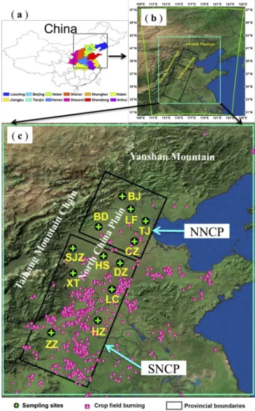
Yanshan and Taihang mountains surround the NCP in the north and west (Fig. 1c). Such topography affects air pollu-tion though the planetary boundary layer (PBL) in complex ways (Miao et al., 2015; Sun et al., 2013; Liu et al., 2009). Hu et al. (2014) reported that the Loess Plateau and NCP result in a mountain–plains solenoid circulation,
exacerbat-Figure 1.The study area, sampling sites and crop fires.(a)The research domain and related provinces in China.(b)Topographical conditions of North China Plain.(c)Location of sampling sites and crop field burning captured by MODIS during the haze episode. Green crosses indicate the sampling sites, and the CFB are shown by the pink dots.
ing air pollution over NCP. Chen et al. (2009) found that a mountain chimney effect is dominated by mountain-valley breeze, enhancing the surface air pollution in Beijing. The mountain–plain breeze develops frequently in Beijing and may play important roles in modulating the local air quality (Miao et al., 2015; Hu et al., 2014; Chen et al., 2009). Miao et al. (2016) found that the mountains played a significant role in the sea–land aerosol circulation and the pollutants could be transported and accumulated in the NCP areas along the mountains, which is treated as the blocking effect (Zhao et al., 2015).
average PM2.5 concentrations are much higher than class
II standard in both the southern NCP (SNCP) and northern NCP (NNCP). The characteristics of the air pollution were analyzed based on PM2.5concentration. Depending on the
satellite-based observations of Moderate Resolution Imag-ing Spectroradiometer (MODIS), a large number of CFB oc-curred in SNCP, whereas few CFBs ococ-curred in NNCP. A more detailed CFB emission inventory was extracted. There-after we analyzed the regional transport of CFB emissions from the SNCP to NNCP driven by prevailing southerly winds. Under continuous southerly wind conditions, the mountains played an important role in northward transport, and caused an accumulation of the aerosol pollutants at the foothills of the mountains. We also analyzed the impact of mountains (especially the Taihang Mountains and the Yan-shan Mountains) on the air pollution transport.
2 Description of data 2.1 Geographical location
In order to study the effect of CFB on local and regional air pollution, the research domain is located in eastern China, covering a large regional area (more than 10 provinces) (Fig. 1a). The NCP region is in the middle of the research domain, with two mountains in the north and west. The Yan-shan Mountains are located in the north of NCP with east– west directions, and the Taihang Mountains are located in the west of NCP with southwest–northeast directions (Fig. 1b). Figure 1c displays the distribution of online sampling sites and CFB captured by MODIS during the haze episode. We defined two regions of interests according to CFB occur-rences, topographic conditions, industrial and agricultural developments. One is the northern NCP (NNCP), includ-ing two mega cities (Beijinclud-ing and Tianjin) and the northern part of Hebei province, where few CFBs occurs. Another is the SNCP, where substantial CFB occurred during the haze episode as shown in Fig. 1c. Because of the severe haze prob-lem in the capital city of China (Beijing), one of the main focuses is to study the long-range transport of CFB pollution from SNCP to NNCP.
2.2 Meteorological conditions
The reanalysis meteorological data, including wind di-rection, wind speed and planetary boundary layer height (PBLH) were obtained from the European Centre for Medium-range Weather Forecasts (ECMWF), with a spa-tial resolution of 0.125◦
×0.125◦. The data are available at
http://www.ecmwf.int/products/data/. The average wind di-rection and wind speed are displayed in Table 1. During the haze episode, the mean wind directions are 174.8◦ in
NNCP and 165.2◦ in SNCP, and the average wind speeds
are 2.4 m s−1in both NNCP and SNCP. The results suggest
that the prevailing winds are continuous southerly winds with
weak wind speeds, which are favorable to long-range trans-port of pollution from SNCP to NNCP, which has been re-ported as one of the major contributors to haze formation in the Beijing City (Tie et al., 2015).
2.3 PM2.5measurements
The hourly PM2.5 mass concentrations were continuously
monitored by the Ministry of Environmental Protection (MEP) of China (http://datacenter.mep.gov.cn), including five sites in NNCP and seven sites in SNCP (indicated by green crosses in Fig. 1c). The data were updated from the website: http://www.pm25.in/. Table 1 summarizes the site information and the observed PM2.5 concentrations.
Dur-ing the study period, the average PM2.5 concentrations are
200.0 µg m−3in NNCP and 184.1 µg m−3in SNCP. The
mea-sured PM2.5 concentrations are much higher than a class
II standard (daily mean of 75 µg m−3), indicating an
occur-rence of a heavy pollution event. We analyzed the charac-teristics of the air pollution based on the PM2.5
concentra-tion simulated by WRF-CHEM. Meanwhile, it is worth not-ing that the highest PM2.5concentrations occurred along the
foothill sites of the Taihang Mountains. At the foothill sites of Beijing, Baoding, Shijiazhuang and Xingtai, PM2.5
concen-trations are 245.5, 287.7, 257.9 and 320.1 µg m−3,
respec-tively. The mean PM2.5concentration in these four sites is
277.8 µg m−3, much higher than 147.2 µg m−3averaged from
the other sites. Considering the continuous southerly winds and the topographic conditions, we studied the impact of the mountains on the air pollution transport.
3 Methods
3.1 Model description
We used Weather Research and Forecasting Chemical model (WRF-CHEM) (Grell et al., 2005) to simulate the spatial and temporal variability of PM2.5 concentration. The
Table 1.The average PM2.5concentration, wind direction and wind speed of the observations from 12:00 to 00:00 LT on 6 to 12 Oct. The
sampling sites located at the foot of mountains are emphasized in bold.
Region Site Longitude Latitude PM2.5 Wind dir. Wind spd. (◦E) (◦N) (µg m−3) (◦) (m s−1)
NNCP Beijing (BJ) 116.41 40.04 245.5 185.8 2.2 Langfang (LF) 116.73 39.56 214.7 177.0 2.4 Tianjin (TJ) 117.31 39.09 134.7 173.5 2.4
Baoding (BD) 115.49 38.87 287.7 171.2 2.2 Cangzhou (CZ) 116.87 38.31 117.3 166.6 2.5
200.0 174.8 2.35
SNCP Shijiazhuang (SJZ) 114.49 38.04 257.9 175.2 2.0 Hengshui (HS) 115.68 37.74 166.7 163.7 2.6 Dezhou (DZ) 116.31 37.47 152.4 162.7 2.6
Xingtai (XT) 114.50 37.09 320.1 198.1 2.3 Liaocheng (LC) 116.00 36.46 139.7 158.4 2.6 Hezhe (HZ) 115.46 35.26 105.0 138.9 2.4 Zhengzhou (ZZ) 113.66 34.79 146.9 159.2 2.4
184.1 165.2 2.42
ammonia–sulfate–nitrate–chloride–water aerosols and their gas-phase precursors of H2SO4–HNO3–NH3–HCl–water
va-por. The Yonsei University (YSU) PBL scheme (Hong et al., 2006), Lin microphysics scheme (Lin et al., 1983) and Noah land-surface model (Chen and Dudhia, 2001) were utilized. The model has been successfully applied in several regional pollution studies (Tie et al., 2009, 2007; He et al., 2015).
The WRF-CHEM model is configured with resolution of 6 km×6 km (200×300 grid cells) centered in (117◦E,
39◦N). Vertical layers extend from the surface to 50 hPa,
with 28 vertical layers, involving seven layers in the bottom of 1 km. The meteorological initial and boundary conditions were gathered from NCEP FNL (National Centers for En-vironmental Prediction Final) Operational Global Analysis data. The lateral chemical initial conditions were constrained by a global chemical transport model – MOZART4 (Model for Ozone and Related chemical Tracers, version 4) – 6 h out-put (Emmons et al., 2010; Tie et al., 2005). For the episode simulations, the spin-up time of the WRF-CHEM model is 3 days.
The surface emission inventory used in this study was obtained from the Multi-resolution Emission Inventory for China (MEIC) (Zhang et al., 2009), which is an update and improvement for the year 2010 (http://www.meicmodel.org). The emission inventory estimated only anthropogenic emis-sion such as non-residential sources (transportation, agricul-ture, industry and power) and residential sources related to fuel combustions. The biogenic emissions are calculated on-line with the WRF-CHEM model using the MEGAN model (Guenther et al., 2006). Additionally, we added emission from CFB in the present study.
Figure 2.The(a)yearly and(b)monthly CFB observed by MODIS in the research domain during the year of 2008 to 2014.
3.2 Crop field burning emissions
dependence character suggests that the CFB emissions dur-ing October are much larger than annual averages. In or-der to have the detailed horizontal distribution of the pol-lutant emissions of CFB, we elaborated a method to gener-ate emission inventory using the sgener-atellite data of “MODIS Thermal Anomalies/Fire product (MOD/MYD14DL)”. The MOD/MYD14DL product can detect small opening fires (<100 m2)(Giglio et al., 2003) and produce the geographic location of open fire activities (van der Werf et al., 2006). In this study, the CFB was defined as MOD/MYD14DL active fires occurred over the cropland, which is classified by the MODIS Combined Land Cover Type product (Friedl et al., 2010).
First, we estimated the CO emission of CFB, utilizing a widely used method (Streets et al., 2003; Cao et al., 2008; Zhang et al., 2008; Ni et al., 2015) based on the annual provincial statistical data. The provincial emission of crop residues burning can be calculated by Eq. (1):
Ei,CO=
X3
k=1Pi,k×Fi×Dk×Rk×CEk×EFCO, (1)
where i stands for each province and k for different crop species of rice, corn and wheat.Ei,COstands for CO emission
from CFB ofith province in gigagrams [Gg].Pi,kis the yield
of crop in Gg.Fi is the proportion of residues burned in the
field.Dk is the dry fraction of crop residue (dry matter).Rk
is the residue-to-crop ratio (dry matter). CEk is the
combus-tion efficiency and EFCOis the emission factors of CFB. The Pi,k values were taken from an official statistical yearbook
(NBS, 2015) (Table S1 in the Supplement), and the Fi on
a provincial basis were taken from Wang and Zhang (2008) and Zhang Yisheng (Unpublished doctor thesis-in Chinese) (Table S1). The parameters of Dk, Rk and CEk are listed
in Table S2. The EFCO from CFB was summarized range
from 52 to 141 g kg−1in China (Table S3). In this study, we
used 111 g kg−1as the average EF
COof crop residue, which
was used to estimate the emissions from global open burning (Wiedinmyer et al., 2011).
The provincial CO emission was temporally and spa-tially allocated according to the CFB activities. The detailed daily CO emission ofkth grid (Ek,CO)was calculated using
Eq. (2): Ek,CO=FCk
FCi ×
Ei,CO, (2)
where FCk and FCi are the total CFB fire counts inkth grid
andith province, respectively (Table S1).
Thereafter, the emissions of various gaseous and particu-late species (Espec1)were calculated by the Eq. (3).
Further-more, individual chemical compounds (Espec2)were
calcu-lated by Eq. (4):
Ek,spec1=EFspec1
EFCO ×
Ek,CO, (3)
Ek,spec2=Ek,NMOC×scale, (4)
where Ek,spec1 and Ek,spec2 are the kth grid emission of
the specify WRF-CHEM species,Espec1 and EFCO are the
emission factors of CFB, Ek,NMOC is NMOC emission in
thekth grid calculated by Eq. (3) and scale is the value to convert NMOC emissions to WRF-CHEM chemical species. The emission factors for gaseous and particulate species and scale to convert NMOC emissions to WRF-CHEM chemical species from CFB were taken from available data sets (Wied-inmyer et al., 2011; Akagi et al., 2011; Andreae and Merlet, 2001), which were summarized by Wiedinmyer et al. (2011) (Table 2).
4 Results and discussions
4.1 Evaluate the crop field burning emission
The provincial CO emissions of CFB were estimated based on Eq. (1), and there was 8.2 Tg CO emitted from CFB in 2014 (Table S1). This result is comparable to previous stud-ies, which were 4.6–10.1 Tg yr−1(Cao et al., 2008; Ni et al.,
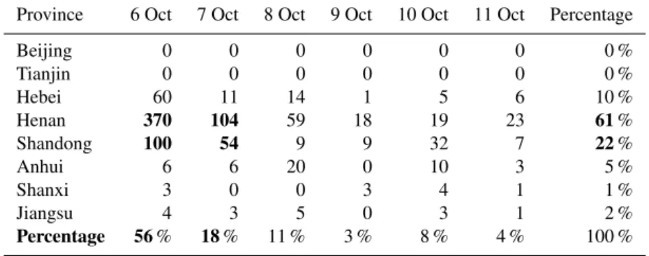
2015; Streets et al., 2003; Yan et al., 2006). According to the MODIS observations, a large number of CFB occurred in SNCP, including the provinces of Henan with 61 % and Shandong with 22 %. Most of CFB occurred on 6 and 7 Oc-tober, accounting for 75 % (Table 3).
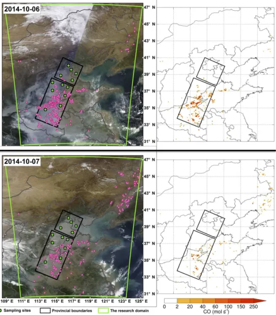
Table 4 shows the CFB emissions of gaseous and partic-ulate species on 6 and 7 October, including the mega cities of Beijing and Tianjin, and provinces of Hebei, Henan and Shandong in NCP. Figure 3 displays the CFB activities and related CO emission on 6 and 7 October. Most of the pollu-tants are emitted from Henan in SNCP, accounting for 73 % on 6 October and 65 % on 7 October. Plenty of pollutants emitted from CFB on 6 October, producing more than 5.1 Gg PM2.5and 98.0 Gg CO (1 Gg=109g).
4.2 Statistical characteristics of the evaluation
The characteristics of the haze pollution were defined by PM2.5 concentration, which is significantly affected by the
local wind fields and PBLH in the NCP region (Tie et al., 2015). In order to evaluate the model performance, the model simulations were compared with the measured results in both species concentrations (PM2.5, O3 and NO2)and
Table 2.The gaseous and particulate species emission factors (g kg−1)and scales to convert NMOC emissions (kg day−1)to WRF-CHEM
chemical species (moles-species day−1)from crop field burning. The detailed chemical species are described by Stockwell et al. (1990).
Gaseous species Particulate species COa NOxa NOa NOb2 SO2c NHa3 NMOCa OCc BCc PM2.5a
111 3.5 1.7 3.9 0.4 2.3 57 3.3 0.69 5.8 Chemical-compounds-to-NMOC scalesa,b
ETH HC3 HC5 OL2 OLT OLI TOL CSL HCHO ALD KET ORA2 ISO 0.43 0.73 0.07 1.09 0.27 0.20 1.07 0.49 1.84 3.05 0.83 2.19 0.60
aThe values were taken from Andreae and Merlet (2001).bThe values were taken from Wiedinmyer et al. (2011).cThe values were taken from
Akagi et al. (2011).
Table 3. The fire counts of crop field burning detected by the MODIS in the provinces over NCP during the haze episode (from 6 to 11 October 2014).
Province 6 Oct 7 Oct 8 Oct 9 Oct 10 Oct 11 Oct Percentage
Beijing 0 0 0 0 0 0 0 %
Tianjin 0 0 0 0 0 0 0 %
Hebei 60 11 14 1 5 6 10 % Henan 370 104 59 18 19 23 61% Shandong 100 54 9 9 32 7 22%
Anhui 6 6 20 0 10 3 5 %
Shanxi 3 0 0 3 4 1 1 %
Jiangsu 4 3 5 0 3 1 2 %
Percentage 56% 18% 11 % 3 % 8 % 4 % 100 %
NMB=
PN
i=1(Pi−Oi)
PN i=1Oi
, (5)
R=
PN
i=1(Pi−P )(Oi−O)
h PN
i=1(Pi−P ) 2PN
i=1(Oi−O) 2i
1 2
, (6)
wherePi is the predicted results and Oi represents the
re-lated observations. N is the total number of the predictions used for comparisons. Meanwhile,P andOare the average prediction and related mean observation, respectively.
Figure 4 shows the measured and calculated temporal vari-ations of regional average species concentrvari-ations, including PM2.5, O3 and NO2. The WRF-CHEM model reproduced
the pollution episode well, with a good agreement with ob-servations. The R of simulated and measured PM2.5
con-centrations are 0.88 in both NNCP and SNCP (Fig. 4a). The simulations are overall lower than the observations with NMB of −12 % in NNCP and −7 % in SNCP.
Consider-ing the high average PM2.5concentration with 200.0 µg m−3
in NNCP and 184.1 µg m−3 in SNCP, obvious
underesti-mates exist with the overall concentrations of 24.0 µg m−3
in NNCP and 12.9 µg m−3in SNPC. This may be related to
the CMAQ (version 4.6) aerosol module, which is likely to
underestimated OM (Organic Matter) due to the uncertainty in secondary organic aerosols mechanism (Baek et al., 2011). Meanwhile, the underestimates are also related to the nega-tive bias in S3, which may be related to cloud contamination (Fig. S1 in the Supplement). Whereas this has only a few impacts on the estimation of CFB contributions since few CFBs occurred during S3. The simulations of O3and NO2
also agree well with observations, withR greater than 0.77 and absolute NMB lower than 17 % (Fig. 4b and c). Figure 5 displays the measured and calculated temporal variations of regional average meteorological parameters, including wind speed, wind direction, and the PBLH. The comparisons be-tween simulated and observed wind fields show good agree-ments in both NNCP and SNCP (Fig. 5a and b), withR all higher than 0.64, and the absolute NMB is no more than 15 %. Meanwhile, theR of PBLH is larger than 0.88 and the absolute NMB is no more than 10 % (Fig. 5c).
4.3 Characteristics of the heavy pollution events
According to the evolution of PM2.5concentration (Fig. 4a),
Table 4.The emissions (Gg day−1)of gaseous and particulate species from crop field burning on 6 and 7 October in NCP region, including
the provinces of Beijing, Tianjin, Hebei, Henan and Shandong.
Time Province CO NOx NO NO2 NMOC SO2 NH3 PM2.5 OC BC
6 Oct Beijing 0.00 0.00 0.00 0.00 0.00 0.00 0.00 0.00 0.00 0.00 Tianjin 0.00 0.00 0.00 0.00 0.00 0.00 0.00 0.00 0.00 0.00 Hebei 10.58 0.33 0.16 0.37 5.44 0.04 0.22 0.55 0.31 0.07 Henan 71.17 2.24 1.09 2.50 36.55 0.26 1.47 3.72 2.12 0.44 Shandong 16.27 0.51 0.25 0.57 8.35 0.06 0.34 0.85 0.48 0.10 Total 98.0 3.1 1.5 3.4 50.3 0.4 2.0 5.1 2.9 0.6 7 Oct Beijing 0.00 0.00 0.00 0.00 0.00 0.00 0.00 0.00 0.00 0.00 Tianjin 0.00 0.00 0.00 0.00 0.00 0.00 0.00 0.00 0.00 0.00 Hebei 1.94 0.06 0.03 0.07 1.00 0.01 0.04 0.10 0.06 0.01 Henan 20.01 0.63 0.31 0.70 10.27 0.07 0.41 1.05 0.59 0.12 Shandong 8.79 0.28 0.13 0.31 4.51 0.03 0.18 0.46 0.26 0.05 Total 30.7 1.0 0.5 1.1 15.8 0.1 0.6 1.6 0.9 0.2
The major characteristics of each stage are briefly summa-rized below. Related simulations in bracket follow the de-tailed observations.
– S1 (pollution formation): it is dominated by a contin-uous southerly wind, with a mean wind speed of 2.5 (2.7) m s−1in NNCP and 3.0 (3.6) m s−1in SNCP. The
backward trajectories, with the HYSPLIT model on-line version, of Beijing, Tianjin and Baoding during S1 reflected how the CFB influenced the NNCP region (Fig. 6). The air mass mainly came from the south, originating from the SNCP region. The pollutants are continuously transported from SNCP to NNCP, leading to pollutants accumulation in NNCP, which is charac-terized by the steady rising of PM2.5 concentration in
NNCP from 20.6 (41.0) µg m−3(at 12:00, 6 October) to
242.7 (217.5) µg m−3(at 00:00 LT on 8 October) (Fig. 4
a1).
– S2 (pollution outbreak): during S2, the air pollution deteriorates. It is a relative stable period of heavy pollution with average PM2.5 concentration of 252.0
(241.2) µg m−3 in NNCP and 214.1 (235.0) µg m−3 in
SNCP, which are higher than those in other stages. This phenomenon may be related to the relatively lower wind speed and PBLH.
– S3 (pollution clear): during S3, the southerly winds gradually decrease, and turn to northerly winds at the end of S3. Clean airs from the north region of China obviously improve the air quality. Compared with S2, the average PM2.5concentrations are decreased in both
NNCP and SNCP.
There were several important issues shown in the results, and should be addressed. (1) The PM2.5concentrations are
extremely high during the S2 period, and the daily average
concentrations are greater than the Chinese National Stan-dard (75 µg m−3)by 2–3 times. (2) The air pollution is
se-vere in a large region (occurred in both NNCP and SNCP). (3) During the S1 and S2 periods, there is a time lag between SNCP and NNCP for PM2.5concentrations. Because it is a
continuous southerly wind condition, it shows the important impact of long-range transport of PM2.5particles from the
SNCP to NNCP.
4.4 Contributions of crop field burning
Model sensitivity studies were conducted to separate the in-dividual CFB contribution. Two model simulations were per-formed, i.e., one with both anthropogenic and CFB emissions while the other with only anthropogenic emission. We calcu-lated PM2.5 distributions by including CFB emissions
(an-thropologic and CFB) and excluding CFB emissions (only anthropologic). In this study, the CFB contributions were quantified by regional average contribution in mass concen-tration (CPM2.5)and daily average contribution proportion
(PPM2.5):
CPM2.5=TPM2.5−APM2.5, (7)
PPM2.5=CPM2.5
TPM2.5
, (8)
where TPM2.5 represents the simulated PM2.5
concentra-tions considering total emission; APM2.5 denotes the
sim-ulated PM2.5concentrations only considering anthropologic
emissions. CPM2.5and TPM2.5are daily average value for
CPM2.5and TPM2.5, respectively.
Figure 7 displays the regional observed and simulated PM2.5 concentrations considering total emissions
Figure 3.CFB captured by MODIS with the background of MODIS real-time true color map (left) and related CO emission (right) on 6 and 7 October.
Table 5. Average contribution proportion of crop field burning to PM2.5concentration.
Region 6 Oct 7 Oct 8 Oct 9 Oct 10 Oct 11 Oct NNCP 5 % 32% 10% 3 % 2 % 4 % SNCP 34% 17% 6 % 3 % 1 % 1 %
also proved by the daily PPM2.5of CFB (Table 5). The high
values of PPM2.5 in SNCP appear on 6 October with 34 %
and on 7 October with 17 %, when plenty of CFB occurred. Simultaneously, the high values of PPM2.5in NNCP appear
on 7 October with 32 % and 8 October with 10 %, showing a later occurrence than that in SNCP. The time lag suggests that the plume with CFB may be transported from SNCP to NNCP.
The detailed hourly CFB contributions to PM2.5
concen-trations (CPM2.5) are displayed in Fig. 8. The values of
CPM2.5 in NNCP are generally lag synchronized with that
in SNCP, such asPN1 versus PS1 and PN2 versus toPS2
(Fig. 8a and b). Apparently, the lagged time is not constant and varied with the wind fields. The specific details perform relaxed lag synchronized, especially between thePN2 and PS2. This phenomenon further indicates that the CFB
contri-bution in SNCP is mainly due to local emission, whereas the CFB contribution in NNCP is largely a result of long-range transport from SNCP. Indeed, the CFB pollution plume goes through a long-range transport to NNCP can cause an obvi-ous increase to PM2.5concentration, with the maximum daily
Figure 4.Regional average temporal variations in simulated (in red) and observed (in blue) results of species concentrations of(a)PM2.5
(b)O3and(c)NO2over the regions of NNCP and SNCP.
Figure 6. Backward trajectories of NNCP (Beijing, Tianjin and Baoding) during S1 (12:00–00:00 LT on 6–8 Oct) in different heights of 100, 500 and 1000 m.
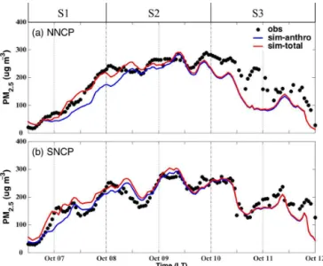
Figure 7. Hourly PM2.5 concentration of observations (obs) and
simulations (sim-total and sim-anthro) in(a)NNCP and(b)SNCP; “sim-total” represents the simulations considering total emissions (anthropologic and crop field burning), whereas “sim-anthro” is the simulations only considering anthropologic emissions.
Figure 8.CFB contribution to PM2.5concentration (CPM2.5)(a)in
SNCP,(b) in NNCP and(c)their comparison. The key point-in-local-times of T1 (23:00, 6th), T2 (05:00, 7th), T3 (20:00, 7th) and T4 (19:00, 8th) are signed with blue arrow.
the significant local pollution sources, but also a considerable regional pollution source.
To clearly show the time evolution of the CFB effect on PM2.5 concentration, four time points were defined in
Fig. 8c, such as T1 (23:00, 6 Oct), T2 (05:00, 7 Oct), T3 (20:00, 7 Oct) and T4 (19:00, 8 Oct). At T1, prominent CFB contribution occurred in SNCP with the highest value of 71.9 µg m−3, but accompanied with unimportant CFB
con-tribution in NNCP with a low value of 7.7 µg m−3. At T2,
the CFB contribution in SNCP decline with a relatively high value of 44.2 µg m−3, but a rise in NNCP with 51.6 µg m−3
(near the transition between P1 and P2). At T3, the CFB con-tribution rapidly decreases to a low value of 24.0 µg m−3in
SNCP, but increase to the highest with 47.0 µg m−3in NNCP.
At T4, the CFB contributions largely decrease, becoming lesser in both SCNP (9.1 µg m−3)and NNCP (11.4 µg m−3).
Interestingly, the CFB contribution in SNCP drops faster than that in NNCP (P2 in Fig. 8c), resulting in stronger effects in NNCP than in SNCP, as well as longer effects in NNCP.
To further understand the evolution of CFB to heavy haze pollution, we analyzed the horizontal distributions of PM2.5 concentration (TPM2.5) and related CFB
contribu-tion (CPM2.5)at T1, T2, T3 and T4 (Fig. 9). The pattern
comparisons between simulated and observed near-surface PM2.5 concentrations (TPM2.5) perform well (Fig. 9, left
Figure 9.The distributions of TPM2.5and CPM2.5of the key point-in-local-times of T1, T2, T3 and T4, which represent different pollution
phases of emission from CFB to PM2.5. Left panels also show the pattern comparisons of simulated vs. observed near-surface PM2.5
concentrations (TPM2.5), with PM2.5observations of colored circles. Black arrows denote simulated surface winds.
emitted from CFB in SNCP and the CFB plume had not yet been largely transported to NNCP (see CPM2.5of Fig. 9 T1).
The CFB contribution is high in SNCP with 72.6 µg m−3,
ac-counting for 71 % of the total PM2.5, whereas the CFB
contri-bution is low with 8.1 µg m−3in NNCP, only accounting for
21 %. At T2, high CFB contribution occurred in both SNCP and NNCP with 37 µg m−3, suggesting that plenty of CFB
pollutants were emitted from SNCP and were transported to NNCP (see CPM2.5of Fig. 9 T2). At T3, CFB contribution
Table 6.The regional average contribution of CFB in mass concen-tration and percentage, and the time lag of NNCP to SNCP for the four time points of T1 (23:00, 6 Oct), T2 (05:00, 7 Oct), T3 (20:00, 7 Oct) and T4 (19:00, 8 Oct).
Time Mass (µg m−3) Percentage Lag time (h)
NNCP SNCP NNCP SNCP
T1 8.1 72.6 21 % 71 % 7 T2 36.7 36.5 73 % 27 % 8 T3 50.4 20.2 58 % 13 % 11 T4 13.4 10.3 6 % 5 % 12
noting that the high CFB contribution with 50.4 µg m−3
(58 %) still remained in NNCP (see CPM2.5of Fig. 9 T3).
At T4, the CFB contribution largely decreased in both SNCP and NNCP (no more than 6 %) (see CPM2.5 of Fig. 9 T4).
The time lag of NNCP to SNCP is 7–12 h, and gradually in-creases from T1 to T4, implicating that the effect of CFB re-mains longer in NNCP than in SNCP. The highest PM2.5
con-centrations are along the foothills of the Taihang Mountains (Left panels of Fig. 9), which may be related to the mountain effects.
4.5 Impact of mountains
Sensitivity experiments were conducted to quantify the im-pacts of the Taihang Mountains (referred as R-T), the Yan-shan Mountains (R-Y) and both of them (R-TY) on heavy pollution. The mountains were removed from the model cal-culation, in which the altitude of mountains were reduced to the average altitude of NCP (30 m). With the reduction of altitudes of the topography, the dynamical conditions cal-culated from WRF-CHEM changed, which affect pollution transport, especially along the foothills of mountains. In this study, we utilized the differences between the simulations with or without mountains to represent the effect of the to-pography on PM2.5 concentration, which were calculated
based on Eq. (9). As an online dynamical model, the topogra-phy changes in WRF-CHEM can lead to dynamical changes, such as the wind speeds at the foothills of the mountains. This is a useful and traditional sensitivity analysis method for numerical model to quantify the mountains effects, but with some shortcomings, which are to bring uncertainties to the sensitivity experiment. First, the impact of topography is too complicated to be completely quantified only by the altitude remove behavior. Second, the initial NCEP FNL data with mountains are treated as “real” in scenarios without moun-tains. The sensitive configuration and related enclosing scope are displayed in Fig. S2.
IPM2.5=RPM2.5−TPM2.5, (9)
where IPM2.5 is the net impacts of mountains on PM2.5;
RPM2.5denotes the simulated PM2.5concentration with
re-moval behaviors, involving R-TY, R-T and R-Y; TPM2.5
rep-Figure 10. The elevation contours and the pattern comparisons of simulated vs. observed near-surface PM2.5concentrations from
12:00 to 00:00 LT on 7 to 10 Oct. Colored circles: PM2.5 observa-tions of foothill sites; Colored squares: PM2.5observations of
non-foothill sites; Black arrows: simulated surface winds. The 200 m contour was highlighted with bold black line.
resents the simulated PM2.5concentration considering
emis-sion of anthropologic and CFB, which corresponds to the case of R0 (Fig. S2a).
The sensitivity study period was selected from 12:00 to 00:00 LT on 7 to 10 October. Figure 10 displays the eleva-tion contours and the horizontal distribueleva-tions of PM2.5
con-centration with the effect of mountains, exhibiting a good performance of the pattern comparisons between simulated and observed near-surface PM2.5concentrations. The results
illustrate that the mountains had important impacts on re-gional PM2.5concentration, especially for the region along
the foothills of mountains with a heavy pollution area, cov-ering sampling sites of BJ, BD, SJZ and XT. Here, it is attributed to the mountain blocking effect, which has two categories of influences. First, the mountains block the air-flows, causing pollutant accumulation and resulting in high PM2.5 loading at the foothills of mountains (influence-1,
block). Second, the mountains redirect the airflows, caus-ing the pollutants to move toward the downwind foothill ar-eas (influence-2, redirect). Both influences act to prevent the pollutant plume to disperse toward western mountains, caus-ing accumulations of the air pollutants along the foothills of mountains. These two influences of mountain blocking ef-fects are illustrated as schematic pictures in Fig. S3.
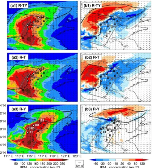
Figure 11 displays the simulated PM2.5concentration due
to the mountain effects (RPM2.5), with the three cases (R-TY,
Figure 11.The average spatial distribution of PM2.5concentration and horizontal winds during 12:00 to 00:00 LT on 7 to 10 Oct.(a)
Simu-lated PM2.5loading with remove behaviors RPM2.5, involving R-TY, R-T and R-Y.(b)The related impacts of mountains on PM2.5(IPM2.5),
which represent the effect of related mountains. The bold black lines were used to stress enclosing scope of each remove behavior.
PM2.5 concentrations increase 40–120 µg m−3 in the
west-ern part of Taihang Mountains, and reduce 20–60 µg m−3in
NCP. The distribution of the reduced pollution plume shows a northeast band plume, indicating the mountain blocking ef-fect. With the removal of the Yanshan Mountains (R-Y), the high PM2.5concentrations still remained along the foothills
of the Taihang Mountains (Fig. 11 a3), but more pollutants are pushed forward along the foothill, toward the northeast-ern NCP. Without the blocking effect of the Yanshan Moun-tains, the PM2.5 concentrations increased 20–80 µg m−3 in
the northern part of the Yanshan Mountains, and decreased 10–60 µg m−3in the southern part of the Yanshan Mountains
(Fig. 11 b3).
In the foothill sampling sites (BJ, BD, SJZ and XT), the average PM2.5 concentrations are reduced 54.2 µg m−3 for
the case of T, which is much higher than the case of R-Y (28.4 µg m−3). For the other non-foothill sites, the
aver-age reduction is 34.7 µg m−3 for the case of R-T, which is
also much higher than the case of R-Y (2.4 µg m−3),
sug-gesting that the Taihang Mountains have stronger effects than the Yanshan Mountains. Meanwhile, the higher impacts in the foothill sampling sites than non-foothill sites are further demonstrated.
5 Conclusions
based on the provincial statistical data and CFB activities captured by MODIS. The WRF-CHEM mode was applied to study the effect of CFB on the PM2.5 concentrations in
NCP, especially the evaluation of CFB plums pollution, such as local influence and long-range transportation. We get some insights of how could CFB affect the air quality in NNCP and Beijing under heavy haze condition, though more and longer studies are needed to get more representative conclusions. The results are summarized:
1. A more detailed CFB emission inventory was generated in NCP. The daily CFB emissions were estimated de-pending on CFB activities captured by MODIS. Plenty of pollutants emitted from SNCP on 6 and 7 October, producing plenty of PM2.5pollution, but few in NNCP
during the entire haze period.
2. The WRF-CHEM model reproduced the pollution episode with a good agreement with observations. The correlation coefficients (R) of simulated and measured PM2.5concentration are 0.88 in both NNCP and SNCP,
and the related NMB are−12 % in NNCP and−7 % in
SNCP. The simulated winds and PBLH are also in good agreement with observations in both NNCP and SNCP. 3. The WRF-CHEM model was used to investigate the
im-pacts of CFB contribution and its evaluation on PM2.5
concentration. The SNCP region is mainly influenced by the local CFB emissions, causing a maximum of 34 % PM2.5 increase. Whereas the NNCP region is
mainly affected by the long-range transport of pollution plume emitted from CFB in SNCP, causing a maximum of 32 % PM2.5increase in NNCP.
4. The research domain includes two regions of interests. One is the NNCP, including two mega cities (Beijing and Tianjin), where few CFBs occurred. Another is the SNCP, where substantial CFB occurred. This study shows that there is a substantially long-range trans-port of CFB plume from SNCP to NNCP. More im-portantly, the effect of CFB remains longer in NNCP than in SNCP along the foothill areas of the Taihang Mountains, causing significant enhancement in Beijing in both time and magnitude.
5. Another major finding is that the mountains, surround-ing the NCP in the north and west, play significant roles in enhancing the PM2.5 pollution in NNCP through
the blocking effect. Mountains block and redirect the airflows, causing the pollution accumulation along the foothills of mountains. The Taihang Mountains had greater impacts on PM2.5 concentration than the
Yan-shan Mountains.
On account of various factors, such as pollutant long-range transport and pollutant accumulation caused by mountain ef-fects, the prohibition of CFB should be strict not only in or around Beijing, but also on the ulterior crop growth areas of SNCP. Other PM2.5emissions in the SNCP should be
6 Data availability
1. The real-time NO2, O3 and PM2.5 are accessible for
the public on the website http://106.37.208.233:20035/. One can also access the historic profile of observed am-bient pollutants through visiting http://www.aqistudy. cn/.
2. The reanalysis meteorological data, including wind di-rection, wind speed and planetary boundary layer height (PBLH) are obtained from the European Centre for Medium-range Weather Forecasts (ECMWF), for the public on the website: http://apps.ecmwf.int/datasets/ data/interim-full-daily/levtype=sfc/.
3. The MODIS Land Cover products are accessible for the public on the website https://lpdaac.usgs.gov/dataset_ discovery/modis/modis_products_table.
4. The MODIS Fire products are accessible for the pub-lic on the website https://firms.modaps.eosdis.nasa.gov/ download/.
5. The MODIS true color map are accessible for the public on the website https://worldview.earthdata.nasa.gov/.
The Supplement related to this article is available online at doi:10.5194/acp-16-9675-2016-supplement.
Acknowledgements. The PBL height and wind field data were ob-tained from the European Centre for Medium-Range Weather Fore-casts (ECMWF) website (http://www.ecmwf.int/products/data/). This work is supported by the National Natural Science Foundation of China (NSFC) under grant nos. 41275186 and 41430424, and the Open Fund of the State Key Laboratory of Loess and Quaternary Geology (SKLLQG1413). The National Center for Atmospheric Research is sponsored by the National Science Foundation. Edited by: H. Su
References
Akagi, S. K., Yokelson, R. J., Wiedinmyer, C., Alvarado, M. J., Reid, J. S., Karl, T., Crounse, J. D., and Wennberg, P. O.: Emis-sion factors for open and domestic biomass burning for use in atmospheric models, Atmos. Chem. Phys., 11, 4039–4072, doi:10.5194/acp-11-4039-2011, 2011.
Andreae, M. O. and Merlet, P.: Emission of trace gases and aerosols from biomass burning, Global Biogeochem. Cy., 15, 955–966, 2001.
Baek, J., Hu, Y., Odman, M. T., and Russell, A. G.: Modeling sec-ondary organic aerosol in CMAQ using multigenerational ox-idation of semi-volatile organic compounds, J. Geophys. Res.-Atmos., 116, D22204, doi:10.1029/2011JD015911, 2011.
Bi, Y., Wang, Y., and Cao, C.: Straw Resource Quantity and its Re-gional Distribution in China [J], Journal of Agricultural Mecha-nization Research, 3, 1-7-, 2010.
Binkowski, F. S. and Roselle, S. J.: Models-3 Community Multiscale Air Quality (CMAQ) model aerosol component 1. Model description, J. Geophys. Res.-Atmos., 108, 4183, doi:10.1029/2001JD001409, 2003.
Cao, G., Zhang, X., Wang, Y., and Zheng, F.: Estimation of emis-sions from field burning of crop straw in China, Chinese Sci. Bull., 53, 784–790, 2008.
Chang, J., Brost, R., Isaksen, I., Madronich, S., Middleton, P., Stockwell, W., and Walcek, C.: A three-dimensional Eulerian acid deposition model: Physical concepts and formulation, J. Geophys. Res.-Atmos., 92, 14681–14700, 1987.
Chen, F. and Dudhia, J.: Coupling an advanced land surface-hydrology model with the Penn State-NCAR MM5 modeling system. Part I: Model implementation and sensitivity, Mon. Weather Rev., 129, 569–585, 2001.
Chen, Y., Zhao, C., Zhang, Q., Deng, Z., Huang, M., and Ma, X.: Aircraft study of mountain chimney effect of Beijing, china, J. Geophys. Res.-Atmos., 114, D08306, doi:10.1029/2008JD010610, 2009.
Cheng, Y., Engling, G., He, K.-B., Duan, F.-K., Ma, Y.-L., Du, Z.-Y., Liu, J.-M., Zheng, M., and Weber, R. J.: Biomass burning contribution to Beijing aerosol, Atmos. Chem. Phys., 13, 7765– 7781, doi:10.5194/acp-13-7765-2013, 2013.
Cheng, Z., Wang, S., Fu, X., Watson, J. G., Jiang, J., Fu, Q., Chen, C., Xu, B., Yu, J., Chow, J. C., and Hao, J.: Impact of biomass burning on haze pollution in the Yangtze River delta, China: a case study in summer 2011, Atmos. Chem. Phys., 14, 4573– 4585, doi:10.5194/acp-14-4573-2014, 2014.
Emmons, L. K., Walters, S., Hess, P. G., Lamarque, J.-F., Pfister, G. G., Fillmore, D., Granier, C., Guenther, A., Kinnison, D., Laepple, T., Orlando, J., Tie, X., Tyndall, G., Wiedinmyer, C., Baughcum, S. L., and Kloster, S.: Description and evaluation of the Model for Ozone and Related chemical Tracers, version 4 (MOZART-4), Geosci. Model Dev., 3, 43-67, doi:10.5194/gmd-3-43-2010, 2010.
Friedl, M. A., Sulla-Menashe, D., Tan, B., Schneider, A., Ra-mankutty, N., Sibley, A., and Huang, X.: MODIS Collection 5 global land cover: Algorithm refinements and characterization of new datasets, Remote Sens. Environ., 114, 168–182, 2010. Giglio, L., Descloitres, J., Justice, C. O., and Kaufman, Y. J.: An
en-hanced contextual fire detection algorithm for MODIS, Remote Sens. Environ., 87, 273–282, 2003.
Grell, G. A., Peckham, S. E., Schmitz, R., McKeen, S. A., Frost, G., Skamarock, W. C., and Eder, B.: Fully coupled “online” chem-istry within the WRF model, Atmos. Environ., 39, 6957–6975, 2005.
Guan, D., Su, X., Zhang, Q., Peters, G. P., Liu, Z., Lei, Y., and He, K.: The socioeconomic drivers of China’s primary PM2.5 emissions, Environ. Res. Lett., 9, 024010, doi:10.1088/1748-9326/9/2/024010, 2014.
Hao, W.-M. and Liu, M.-H.: Spatial and temporal distribution of tropical biomass burning, Global Biogeochem. Cy., 8, 495–503, 1994.
He, H., Tie, X., Zhang, Q., Liu, X., Gao, Q., Li, X., and Gao, Y.: Analysis of the causes of heavy aerosol pollution in Beijing, China: A case study with the WRF-CHEM model, Particuology, 20, 32–40, 2015.
Hong, J., Ren, L., Hong, J., and Xu, C.: Environmental impact as-sessment of corn straw utilization in China, J. Clean. Prod., 30, 1e9, doi:10.1016/j.jclepro.2015.02.081, 2015.
Hong, S.-Y., Noh, Y., and Dudhia, J.: A new vertical diffusion pack-age with an explicit treatment of entrainment processes, Mon. Weather Rev., 134, 2318–2341, 2006.
Hu, X.-M., Ma, Z., Lin, W., Zhang, H., Hu, J., Wang, Y., Xu, X., Fuentes, J. D., and Xue, M.: Impact of the Loess Plateau on the atmospheric boundary layer structure and air quality in the North China Plain: A case study, Sci. Total Environ., 499, 228–237, 2014.
Huang, X., Li, M., Li, J., and Song, Y.: A high-resolution emission inventory of crop burning in fields in China based on MODIS Thermal Anomalies/Fire products, Atmos. Environ., 50, 9–15, 2012.
Jiang, C., Wang, H., Zhao, T., Li, T., and Che, H.: Modeling study of PM2.5pollutant transport across cities in China’s Jing–Jin–
Ji region during a severe haze episode in December 2013, At-mos. Chem. Phys., 15, 5803–5814, doi:10.5194/acp-15-5803-2015, 2015.
Koppmann, R., von Czapiewski, K., and Reid, J. S.: A review of biomass burning emissions, part I: gaseous emissions of carbon monoxide, methane, volatile organic compounds, and nitrogen containing compounds, Atmos. Chem. Phys. Discuss., 5, 10455– 10516, doi:10.5194/acpd-5-10455-2005, 2005.
Li, G., Zhang, R., Fan, J., and Tie, X.: Impacts of black carbon aerosol on photolysis and ozone, J. Geophys. Res.-Atmos., 110, D23206, doi:10.1029/2005JD005898, 2005.
Li, G., Lei, W., Zavala, M., Volkamer, R., Dusanter, S., Stevens, P., and Molina, L. T.: Impacts of HONO sources on the photochem-istry in Mexico City during the MCMA-2006/MILAGO Cam-paign, Atmos. Chem. Phys., 10, 6551–6567, doi:10.5194/acp-10-6551-2010, 2010.
Li, G., Bei, N., Tie, X., and Molina, L. T.: Aerosol ef-fects on the photochemistry in Mexico City during MCMA-2006/MILAGRO campaign, Atmos. Chem. Phys., 11, 5169– 5182, doi:10.5194/acp-11-5169-2011, 2011.
Li, G., Lei, W., Bei, N., and Molina, L. T.: Contribution of garbage burning to chloride and PM2.5in Mexico City, Atmos. Chem.
Phys., 12, 8751–8761, doi:10.5194/acp-12-8751-2012, 2012. Li, L., Wang, Y., Zhang, Q., Li, J., Yang, X., and Jin, J.: Wheat
straw burning and its associated impacts on Beijing air quality, Sci. China Ser. D, 51, 403–414, 2008.
Lin, Y.-L., Farley, R. D., and Orville, H. D.: Bulk parameterization of the snow field in a cloud model, J. Clim. Appl. Meteorol., 22, 1065–1092, 1983.
Liu, S., Liu, Z., Li, J., Wang, Y., Ma, Y., Sheng, L., Liu, H., Liang, F., Xin, G., and Wang, J.: Numerical simulation for the coupling effect of local atmospheric circulations over the area of Beijing, Tianjin and Hebei Province, Sci. China Ser. D, 52, 382–392, 2009.
Lu, Z., Zhang, Q., and Streets, D. G.: Sulfur dioxide and primary carbonaceous aerosol emissions in China and India, 1996–2010, Atmos. Chem. Phys., 11, 9839–9864, doi:10.5194/acp-11-9839-2011, 2011.
Miao, Y., Liu, S., Zheng, Y., Wang, S., and Chen, B.: Numerical study of the effects of topography and urbanization on the local atmospheric circulations over the Beijing-Tianjin-Hebei, China, Adv. Meteorol., 2015, 1–16, doi:10.1155/2015/397070, 2015. Miao, Y., Liu, S., Zheng, Y., and Wang, S.: Modeling the
feed-back between aerosol and boundary layer processes: a case study in Beijing, China, Environ. Sci. Pollut. R., 23, 3342–3357, doi:10.1007/s11356-015-5562-8, 2016.
Mukai, S., Yasumoto, M., and Nakata, M.: Estimation of biomass burning influence on air pollution around Beijing from an aerosol retrieval model, Thescientificworldjo., 2014, 1–10, doi:10.1155/2014/649648, 2014.
National Bureau of Statistics (NBS), China Statistical Yearbook 2014, China Statistics Press, Beijing, available at: http://www. stats.gov.cn/tjsj/ndsj/2015/indexch.htm, 2015.
Ni, H., Han, Y., Cao, J., Chen, L.-W. A., Tian, J., Wang, X., Chow, J. C., Watson, J. G., Wang, Q., and Wang, P.: Emission characteris-tics of carbonaceous particles and trace gases from open burning of crop residues in China, Atmos. Environ., 123, 399–406, 2015. Qin, S.-G., Ding, A., and Wang, T.: Transport pattern of biomass burnings air masses in Eurasia and the impacts on China, China Environ. Sci., 26, 641–645, 2006.
Shi, T., Liu, Y., Zhang, L., Hao, L., and Gao, Z.: Burning in agricul-tural landscapes: an emerging naagricul-tural and human issue in China, Landscape Ecology, 29, 1785-1798, 2014.
Shon, Z.-H.: Long-term variations in PM2.5emission from open
biomass burning in Northeast Asia derived from satellite-derived data for 2000–2013, Atmos. Environ., 107, 342–350, 2015. Song, Y., Tang, X., Xie, S., Zhang, Y., Wei, Y., Zhang, M., Zeng, L.,
and Lu, S.: Source apportionment of PM2.5in Beijing in 2004,
J. Hazard. Mater., 146, 124–130, 2007.
Stockwell, W. R., Middleton, P., Chang, J. S., and Tang, X.: The sec-ond generation regional acid deposition model chemical mecha-nism for regional air quality modeling, J. Geophys. Res.-Atmos., 95, 16343–16367, 1990.
Streets, D., Yarber, K., Woo, J. H., and Carmichael, G.: Biomass burning in Asia: Annual and seasonal estimates and at-mospheric emissions, Global Biogeochem. Cy., 17, 1099, doi:10.1029/2003GB002040, 2003.
Su, J., Zhu, B., Kang, H., Wang, H., and Wang, T.: Applications of pollutants released form crop residues at open burning in Yangtze River Delta region in air quality model, Environ. Sci., 33, 1418– 1424, 2012.
Sun, Y., Song, T., Tang, G., and Wang, Y.: The vertical distribution of PM2.5and boundary-layer structure during summer haze in Beijing, Atmos. Environ., 74, 413-421, 2013.
Tie, X., Madronich, S., Walters, S., Zhang, R., Rasch, P., and Collins, W.: Effect of clouds on photolysis and oxi-dants in the troposphere, J. Geophys. Res.-Atmos., 108, 4642, doi:10.1029/2003JD003659, 2003.
Tie, X., Madronich, S., Li, G., Ying, Z., Zhang, R., Garcia, A. R., Lee-Taylor, J., and Liu, Y.: Characterizations of chemical ox-idants in Mexico City: A regional chemical dynamical model (WRF-CHEM) study, Atmos. Environ., 41, 1989–2008, 2007. Tie, X., Geng, F., Peng, L., Gao, W., and Zhao, C.: Measurement
and modeling of O3variability in Shanghai, China: Application
of the WRF-CHEM model, Atmos. Environ., 43, 4289–4302, 2009.
Tie, X., Zhang, Q., He, H., Cao, J., Han, S., Gao, Y., Li, X., and Jia, X. C.: A budget analysis of the formation of haze in Beijing, Atmos. Environ., 100, 25–36, 2015.
van der Werf, G. R., Randerson, J. T., Giglio, L., Collatz, G. J., Kasibhatla, P. S., and Arellano Jr., A. F.: Interannual variabil-ity in global biomass burning emissions from 1997 to 2004, At-mos. Chem. Phys., 6, 3423–3441, doi:10.5194/acp-6-3423-2006, 2006.
Wang, L., Xu, J., Yang, J., Zhao, X., Wei, W., Cheng, D., Pan, X., and Su, J.: Understanding haze pollution over the southern Hebei area of China using the CMAQ model, Atmos. Environ., 56, 69– 79, 2012.
Wang, L. T., Wei, Z., Yang, J., Zhang, Y., Zhang, F. F., Su, J., Meng, C. C., and Zhang, Q.: The 2013 severe haze over southern Hebei, China: model evaluation, source apportionment, and policy implications, Atmos. Chem. Phys., 14, 3151–3173, doi:10.5194/acp-14-3151-2014, 2014.
Wang, Q., Shao, M., Liu, Y., William, K., Paul, G., Li, X., Liu, Y., and Lu, S.: Impact of biomass burning on urban air quality estimated by organic tracers: Guangzhou and Beijing as cases, Atmos. Environ., 41, 8380–8390, 2007.
Wang, Q., Shao, M., Zhang, Y., Wei, Y., Hu, M., and Guo, S.: Source apportionment of fine organic aerosols in Beijing, Atmos. Chem. Phys., 9, 8573–8585, doi:10.5194/acp-9-8573-2009, 2009. Wang, L. T., Wei, Z., Yang, J., Zhang, Y., Zhang, F. F., Su,
J., Meng, C. C., and Zhang, Q.: The 2013 severe haze over southern Hebei, China: model evaluation, source apportionment, and policy implications, Atmos. Chem. Phys., 14, 3151–3173, doi:10.5194/acp-14-3151-2014, 2014.
Wang, S. and Zhang, C.: Spatial and temporal distribution of air pollutant emissions from open burning of crop residues in China, Sciencepaper online, 3, 329–333, 2008.
Wang, W., Maenhaut, W., Yang, W., Liu, X., Bai, Z., Zhang, T., Claeys, M., Cachier, H., Dong, S., and Wang, Y.: One–year aerosol characterization study for PM2.5and PM10 in Beijing,
Atmos. Pollut. Res., 5, 554–562, 2014.
Wesely, M.: Parameterization of surface resistances to gaseous dry deposition in regional-scale numerical models, Atmos. Environ., 23, 1293–1304, 1989.
Wiedinmyer, C., Akagi, S. K., Yokelson, R. J., Emmons, L. K., Al-Saadi, J. A., Orlando, J. J., and Soja, A. J.: The Fire INventory from NCAR (FINN): a high resolution global model to estimate the emissions from open burning, Geosci. Model Dev., 4, 625– 641, doi:10.5194/gmd-4-625-2011, 2011.
Yan, X., Ohara, T., and Akimoto, H.: Bottom-up estimate of biomass burning in mainland China, Atmos. Environ., 40, 5262– 5273, 2006.
Yang, H., Liu, M., and Liufu, Y.: Research and simulation of straw crop burning in Anhui and Henan Provinces using CALPUFF, Res. Environ. Sci., 23, 1368–1375, 2010 (in Chinese).
Yang, Y. R., Liu, X. G., Qu, Y., An, J. L., Jiang, R., Zhang, Y. H., Sun, Y. L., Wu, Z. J., Zhang, F., Xu, W. Q., and Ma, Q. X.: Characteristics and formation mechanism of continuous hazes in China: a case study during the autumn of 2014 in the North China Plain, Atmos. Chem. Phys., 15, 8165–8178, doi:10.5194/acp-15-8165-2015, 2015.
Yao, L., Yang, L., Yuan, Q., Yan, C., Dong, C., Meng, C., Sui, X., Yang, F., Lu, Y., and Wang, W.: Sources apportionment of PM2.5
in a background site in the North China Plain, Sci. Total Environ., 541, 590–598, 2016.
Yevich, R. and Logan, J. A.: An assessment of biofuel use and burn-ing of agricultural waste in the developburn-ing world, Global Bio-geochem. Cy., 17, 1095, doi:10.1029/2002GB001952, 2003. Zha, S., Zhang, S., Cheng, T., Chen, J., Huang, G., Li, X., and Wang,
Q.: Agricultural fires and their potential impacts on regional air quality over China, Aerosol Air Qual. Res., 13, 992–1001, 2013. Zhang, H.: A laboratory study on emission characteristics of gaseous and particulate pollutants emitted from agricultural crop residue burning in China, PhD Thesis, Fudan University, China, 2009.
Zhang, L., Liu, Y., and Hao, L.: Contributions of open crop straw burning emissions to PM2.5 concentrations in China, Environ.
Res. Lett., 11, 014014, doi:10.1088/1748-9326/11/1/014014, 2016.
Zhang, Q., Streets, D. G., Carmichael, G. R., He, K. B., Huo, H., Kannari, A., Klimont, Z., Park, I. S., Reddy, S., Fu, J. S., Chen, D., Duan, L., Lei, Y., Wang, L. T., and Yao, Z. L.: Asian emis-sions in 2006 for the NASA INTEX-B mission, Atmos. Chem. Phys., 9, 5131–5153, doi:10.5194/acp-9-5131-2009, 2009. Zhang, Y.-L. and Cao, F.: Is it time to tackle PM2.5air pollutions in
China from biomass-burning emissions?, Environ. Pollut., 202, 217–219, 2015.
Zhang, Z., Gao, J., Engling, G., Tao, J., Chai, F., Zhang, L., Zhang, R., Sang, X., Chan, C.-y., and Lin, Z.: Characteristics and ap-plications of size-segregated biomass burning tracers in China’s Pearl River Delta region, Atmos. Environ., 102, 290–301, 2015. Zhao, L., Leng, Y., Ren, H., and Li, H.: Life cycle assessment for large-scale centralized straw gas supply project, J. Anhui Agri. Sci., 38, 19462–19464, 2010.
Zhao, S., Tie, X., Cao, J., and Zhang, Q.: Impacts of mountains on black carbon aerosol under different synoptic meteorology con-ditions in the Guanzhong region, China, Atmos. Res., 164, 286– 296, 2015.