ACPD
15, 34533–34604, 2015Contribution of soil biogenic NO emissions during
growing season
B. Mamtimin et al.
Title Page
Abstract Introduction
Conclusions References
Tables Figures
◭ ◮
◭ ◮
Back Close
Full Screen / Esc
Printer-friendly Version Interactive Discussion
Discussion
P
a
per
|
Discussion
P
a
per
|
Discussion
P
a
per
|
Discussion
P
a
per
|
Atmos. Chem. Phys. Discuss., 15, 34533–34604, 2015 www.atmos-chem-phys-discuss.net/15/34533/2015/ doi:10.5194/acpd-15-34533-2015
© Author(s) 2015. CC Attribution 3.0 License.
This discussion paper is/has been under review for the journal Atmospheric Chemistry and Physics (ACP). Please refer to the corresponding final paper in ACP if available.
The contribution of soil biogenic NO
emissions from a managed hyper-arid
ecosystem to the regional NO
2
emissions
during growing season
B. Mamtimin1,2, M. Badawy2,3, T. Behrendt2,4, F. X. Meixner2, and T. Wagner1
1
Max Planck Institute for Chemistry, Satellite Research Group, Mainz, Germany 2
Max Planck Institute for Chemistry, Biogeochemistry Department, Mainz, Germany 3
Department of Geography, Faculty of Arts, Ain Shams University, Egypt 4
Max Planck Institute for Biogeochemistry, Jena, Germany
Received: 16 November 2015 – Accepted: 24 November 2015 – Published: 10 December 2015
Correspondence to: B. Mamtimin ([email protected])
ACPD
15, 34533–34604, 2015Contribution of soil biogenic NO emissions during
growing season
B. Mamtimin et al.
Title Page
Abstract Introduction
Conclusions References
Tables Figures
◭ ◮
◭ ◮
Back Close
Full Screen / Esc
Printer-friendly Version Interactive Discussion
Discussion
P
a
per
|
Discussion
P
a
per
|
Discussion
P
a
per
|
Discussion
P
a
per
|
Abstract
A study was carried out to understand the contributions of soil biogenic NO emis-sions from managed (fertilized and irrigated) hyper-arid ecosystem in NW-China to the regional NO2emissions during growing season. Soil biogenic NO emissions were quantified by laboratory incubation of corresponding soil samples. We have
devel-5
oped the Geoscience General Tool Package (GGTP) to obtain soil temperature, soil moisture and biogenic soil NO emission at oasis scale. Bottom-up anthropogenic NO2 emissions have been scaled down from annual to monthly values to compare mean monthly soil biogenic NO2 emissions. The top-down emission estimates have been derived from satellite observations compared then with the bottom-up emission
esti-10
mates (anthropogenic and biogenic). The results show that the soil biogenic emissions of NO2during the growing period are (at least) equal until twofold of the related anthro-pogenic sources. We found that the grape soils are the main summertime contributor to the biogenic NO emissions of study area, followed by cotton soils. The top-down and bottom-up emission estimates were shown to be useful methods to estimate the
15
monthly/seasonal cycle of the total regional NO2 emissions. The resulting total NO2 emissions show a strong peak in winter and a secondary peak in summer, provid-ing confidence in the method. These findprovid-ings provide strong evidence that biogenic emissions from soils of managed drylands (irrigated and fertilized) in the growing pe-riod can be much more important contributors to the regional NO2 budget (hence to
20
regional photochemistry) of dryland regions than thought before.
1 Introduction
Atmospheric carbon monoxide, methane, and volatile organic compounds are oxidized by the hydroxyl and other radicals through various catalytic cycles (Crutzen, 1987). In these cycles, nitrogen oxides (NOx) are key catalysts, and their ambient concentrations
25
(Chamei-ACPD
15, 34533–34604, 2015Contribution of soil biogenic NO emissions during
growing season
B. Mamtimin et al.
Title Page
Abstract Introduction
Conclusions References
Tables Figures
◭ ◮
◭ ◮
Back Close
Full Screen / Esc
Printer-friendly Version Interactive Discussion
Discussion
P
a
per
|
Discussion
P
a
per
|
Discussion
P
a
per
|
Discussion
P
a
per
|
des et al., 1992). The present evolution of anthropogenic as well as biogenic NOx sources triggers a potential increase of global tropospheric O3concentrations. NOx in
the troposphere originate mostly as NO, which photo-stationary equilibrates with NO2 within a few minutes. According to recent estimates (Kasibhatla et al., 1993; Davidson and Kingerlee, 1997; Denman et al., 2007; Feig et al., 2008), anthropogenic sources
5
amount to 45–67 % of the mid 2000s total global NOx emissions (42–47 Tg a−1, in terms of mass of N). Other globally important sources are soil biogenic NO emission (10–40 %), biomass burning (13–29 %) and lightning (5–16 %). The considerable un-certainty about the range of soil biogenic NO emissions stems from widely differing estimates of the NO emission. Based on field measurements world-wide Davidson and
10
Kingerlee (1997) estimated the global NO soil source strength to be 21 Tg a−1 (with an error margin of 4 to 10 Tg a−1, 40 % of the total), while the 4th IPCC estimate is 8.9 Tg a−1 (Denman et al., 2007) up from the 3th IPCC estimate of 5.6 Tg a−1 (IPCC, 2001). Moreover, the uncertainties in the NO emission data from semi-arid, arid, and hyper-arid regions are very large (mainly due to a very small number of measurements
15
being available). In this context, one should be aware, that approximately 40 % of planet Earth’s total land surface consists of semi-arid, arid and hyper-arid land and more than 30 % of the world’s inhabitants live in hyper-arid, arid and semiarid regions (Lai, 2001). In many parts of the world’s drylands land-cover is strongly changing due to the en-croachment of desert by bushy vegetation (desert→dryland farming; bushy→dryland 20
farming). This leads and will lead to dramatic changes in soil microbial production and consumption of NO. Consequently, it will have a strong impact on the (at least) regional budgets of those reactive trace gases (NOx, O3, volatile organic compounds (VOC), etc.) which involved in the tropospheric oxidizing capacity. For this reason, it is neces-sary to quantify the NO emissions from both, natural and agricultural managed soils of
25
the drylands.
emit-ACPD
15, 34533–34604, 2015Contribution of soil biogenic NO emissions during
growing season
B. Mamtimin et al.
Title Page
Abstract Introduction
Conclusions References
Tables Figures
◭ ◮
◭ ◮
Back Close
Full Screen / Esc
Printer-friendly Version Interactive Discussion
Discussion
P
a
per
|
Discussion
P
a
per
|
Discussion
P
a
per
|
Discussion
P
a
per
|
ted along with NO. In addition, NO production from the HONO photolysis in day time is attributed to the total production of NOxemission. Therefore, it is meaningful to include
HONO emissions to any estimates of biogenic total reactive nitrogen emissions from soil.
The biogenic emission of NO (as well as HONO) depends crucially on soil
temper-5
ature and soil moisture, because these factors affect the availability of organic com-pounds and the microbial activity in the soil (Conrad, 1996; Meixner and Yang, 2006; Ludwig et al., 2001; Oswald et al., 2013). Sufficient soil moisture, high soil tempera-tures, and regular supply of nutrients (N containing fertilizer) are optimum conditions for soil biogenic NO (and HONO) emissions, particularly from arid and hyper-arid land.
10
An oasis is an agriculturally used area in a desert region. The intensification (eco-nomically driven) of oasis agriculture, however, needs enlargement of the arable land area, enhancement of necessary irrigation, and increase of fertilizer use, which leads inevitably to increasing soil biogenic NO (and HONO) emissions. Microbial processes, which underlay NO production (and NO consumption) in soils (e.g., nitrification,
den-15
itrification) are confined to the uppermost soil layers (<0.05 m depth, Rudolph et al., 1996). The most direct method for the characterization of these processes and the quantification of the NO (and HONO) release from soils is usually realized by labora-tory incubation of soil samples taken from top soil layers. In those laboralabora-tory incubation systems, the net release rate of NO is determined from the NO concentration diff
er-20
ence between incoming and outgoing air. The application of this method in the past has proved that the release of NO can be described by specific and unique functions of soil moisture, soil temperature, and ambient NO concentration (Otto et al., 1996; van Dijk et al., 2002; Meixner and Yang, 2006; Feig et al., 2008; Behrendt et al., 2014; Mamtimin et al., 2015).
25
Due to the industrialization of Chinese drylands and also to the intensification of their agriculture, not only large anthropogenic NOx emissions from growing oasis cities are
ACPD
15, 34533–34604, 2015Contribution of soil biogenic NO emissions during
growing season
B. Mamtimin et al.
Title Page
Abstract Introduction
Conclusions References
Tables Figures
◭ ◮
◭ ◮
Back Close
Full Screen / Esc
Printer-friendly Version Interactive Discussion
Discussion
P
a
per
|
Discussion
P
a
per
|
Discussion
P
a
per
|
Discussion
P
a
per
|
the contributions of soil biogenic NO emission of a selected oasis in the Taklimakan desert to the regional NO2emissions during the growing season. For that, we concen-trate (a) on biogenic NO fluxes derived from laboratory incubation measurements of soil samples, (b) on up-scaling the laboratory results to the spatial level of an oasis by a Geoscience General Tool Package (GGTP; specifically developed for all GIS
up-5
scaling procedures of this study), (c) on the estimation of anthropogenic NO2emissions of the oasis based on energy consumption and NO2emission factors of different sec-tors and fuel types, (d) on the quantitative comparison of the derived results to satellite observations (OMI) of the vertical NO2 column densities at regional scale, (e) on the estimation of top-down (satellite derived) and bottom-up (biogenic and anthropogenic)
10
NO2emissions.
2 Materials and methods
2.1 Site description and soil sampling
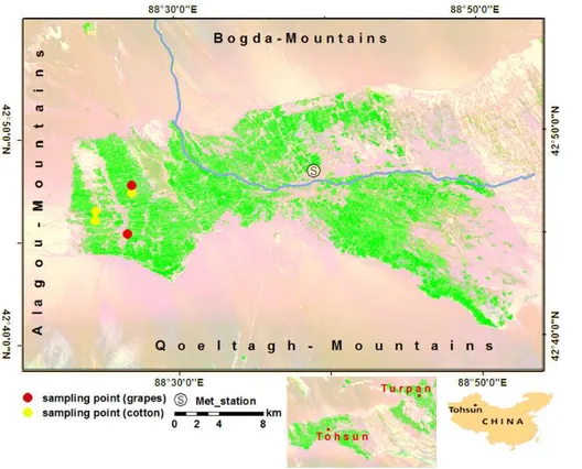
The study area “Tohsun oasis” (Fig. 1) is a hyper-arid region located in the Xinjiang Uyghur Autonomous Region of P.R. China (Mamtimin et al., 2005). The Tohsun oasis
15
belongs administratively to Turpan County with Turpan City as capital (50 km NE from Tohsun oasis). The Tohsun oasis has an extension of 1479 km2, a population of 138 thousand, and topographically constitutes the deepest point of P.R. China (154 m be-low sea-level; Pu, 2011). Major landform types of the Tohsun oasis are sandy-desert and Gobi-desert (stone desert), surrounded on three sides by the mountains of Bogda
20
(north), Qoeltagh (south), and Alagou (west). Topographically, the Tohsun oasis slopes down from northwest to southeast. According to the Koeppen classification (Kottek et al., 2006), the climate of the Tohsun oasis is classified as “cold desert”; i.e. hot summers (July: 33◦C), cold winters (January:−6◦C), and very low precipitation. Mean
annual potential evaporation is about 3400 mm (s. Fig. 2), while the mean annual
pre-25
ACPD
15, 34533–34604, 2015Contribution of soil biogenic NO emissions during
growing season
B. Mamtimin et al.
Title Page
Abstract Introduction
Conclusions References
Tables Figures
◭ ◮
◭ ◮
Back Close
Full Screen / Esc
Printer-friendly Version Interactive Discussion
Discussion
P
a
per
|
Discussion
P
a
per
|
Discussion
P
a
per
|
Discussion
P
a
per
|
The mean monthly precipitation for Tohsun (not shown in Fig. 2) is extremely low: rainfall in June and July is about 2 mm, in January, August, and 1 September mm, re-spectively; and there is no rain for the rest of the year. Agriculture played and plays a significant role in Tohsun oasis; it was one of the most flourishing oases on the an-cient Silk Road (Weggel, 1985). Due to the substantial lack of rainfall, regular dry-land
5
farming is impossible without massive irrigation. Water supplies for irrigated agriculture are dependent on groundwater (pumping-wells), and on the Bai Yanggou River which originates from the Bogda Mountain. The Bai Yanggou River is temporary, defined by the strong seasonal pattern of snow-melt and rain in the mountains (Mamtimin, 2005). Tohsun oasis’ agriculture is dominated by intensive mono-cultivation of grapes and
10
cotton. Grapes from the Turpan country are naturally dried to raisins which are sold on the Chinese internal market and also exported to some Asian countries (Jin, 2011; Pu, 2011). Grapes from Turpan County account for 52 % of grape production in the Xinjiang Uyghur Autonomous Region, and for 20 % of entire China. There, more than 100 small and medium size companies are engaged in raisin processing (Wan, 2012).
15
In 2008, Turpan’s raisin production was 130 000 t which accounted for more than 90 % of all raisins produced in P.R. China (Wan, 2012; Li et al., 2012; Jin, 2011; Pu, 2011). Approximately 40 % of Turpan’s grape production is from the Tohsun oasis (Pu, 2011). To raise the yields of grapes and cotton, the corresponding cultivation techniques have been optimized, which resulted in the application of nitrogen containing fertilizers.
20
Soil samples from the study area were collected in 2010 from a total of three sites of Tohsun’s cotton fields, and from a total of two sites of corresponding grape fields (for sample locations, see Fig. 1). In this study, we also used soil samples from the non-fertilized desert ecosystem as reference, where the desert soil data was adapted from the study Mamtimin et al. (2015).
25
2.2 Remote sensing and accompanying data
In-ACPD
15, 34533–34604, 2015Contribution of soil biogenic NO emissions during
growing season
B. Mamtimin et al.
Title Page
Abstract Introduction
Conclusions References
Tables Figures
◭ ◮
◭ ◮
Back Close
Full Screen / Esc
Printer-friendly Version Interactive Discussion
Discussion
P
a
per
|
Discussion
P
a
per
|
Discussion
P
a
per
|
Discussion
P
a
per
|
formation System (GIS). Landsat images, provided by United States Geological Survey, are widely applicable for purposes like our study because of their rather high spatial resolution (30–15 m). Since the aim of our study is the quantification of biogenic NO emissions from intensively managed arid soils, the consideration of the growth state of the corresponding agro-ecosystems is important. For the representation of the
dif-5
ferent seasons we selected four individual months: April (spring) for the begin, July, August (summer) for the middle, and September (autumn) for the end of the vegeta-tion period. The winter season was not considered, as most of the agro-ecosystems are frozen, hence any microbial activities are negligible. As proposed by many authors (Schott et al., 1985; Markham et al., 1986; Irish, 2003; Chander et al., 2003; Zeng
10
et al., 2004) we derived for each season areal distributions of land surface temperature (LST), soil moisture index (SMI), and land cover types from corresponding satellite data using remote sensing digital image processing. For the selection of Landsat images we confined ourselves to the year 2010 when we have taken the soil samples.
Tropospheric NO2 column densities derived from the OMI satellite instrument
15
(DOMINO version 2.0, Boersma et al., 2011) were used for comparison with the bottom-up emission estimates (biogenic and anthropogenic). OMI is operated in a sun-synchronous orbit such that measurements are taken at about 13:45 LT. The seasonal patterns of satellite derived NO2 column densities were evaluated using cloud-free measurements from 2006 to 2010. Four different areas were selected to represent (1)
20
typical agricultural areas (study area), (2) mixed land use areas (agricultural and small urban), (3) large urban areas, and (4) desert. The seasonal patterns of satellite derived NO2column densities were evaluated using measurements from 2006 to 2010.
For the estimation of anthropogenic sources of NOx, we used fossil fuel consump-tion data from different economic sectors (manufacturing, electricity, transportation and
25
ACPD
15, 34533–34604, 2015Contribution of soil biogenic NO emissions during
growing season
B. Mamtimin et al.
Title Page
Abstract Introduction
Conclusions References
Tables Figures
◭ ◮
◭ ◮
Back Close
Full Screen / Esc
Printer-friendly Version Interactive Discussion
Discussion
P
a
per
|
Discussion
P
a
per
|
Discussion
P
a
per
|
Discussion
P
a
per
|
Traffic Map of Tohsun (1 : 1 050 000, 2010) were involved within this study as additional tools for land use classification.
The meteorological data set (1971–2005) of the Tohsun County Meteorological Sta-tion (42.7833◦N, 88.6500◦E; +1 m a.s.l.) was supplied by the Xinjiang Meteorological Bureau. It contains monthly mean (1971–2005) data of air temperature, precipitation,
5
evaporation, wind speed and direction. Unfortunately, soil moisture content and soil temperature have not been measured routinely at Tohsun County Meteorological Sta-tion.
Satellite derived LST and SMI data, from six individual Landsat images of the Tohsun oasis (25 April, 28 July, 13 and 21 August, 6 and 22 September 2010) were used for
10
the validation of the satellite data by in situ data of soil temperature and soil mois-ture content. Corresponding continuous in situ measurements have been performed with a suitable sensor (MSR®165 data logger; Rotronic, Switzerland) which has been buried at the site of Tohsun County Meteorological Station at 2.5 cm depth between July and September 2010. While soil temperature data was measured directly, data
15
of gravimetric soil water content was calibrated vs. relative humidity of the soil air by a vapor analyzer (VSA, Decagon, USA).
The estimation of the seasonal variation of biogenic NO emissions requires tempo-rally high-resolution data of (a) soil temperature, (b) gravimetric soil water content, and (c) amplification of NO fluxes due to the application of fertilizer (s. Sect. 2.5.2). While
20
soil temperature data could be provided by measurements, data of gravimetric soil moisture content for “cotton” and “grapes” fields had to be assimilated from (a) informa-tion of irrigainforma-tion cycles obtained by personal communicainforma-tion (2010) with farmers in the Tohsun oasis, and (b) from in situ measurements of relative humidity of soil air which were adapted from observations at the oases of Kuche and Minfeng (see Sect. 2.4.5).
25
ACPD
15, 34533–34604, 2015Contribution of soil biogenic NO emissions during
growing season
B. Mamtimin et al.
Title Page
Abstract Introduction
Conclusions References
Tables Figures
◭ ◮
◭ ◮
Back Close
Full Screen / Esc
Printer-friendly Version Interactive Discussion
Discussion
P
a
per
|
Discussion
P
a
per
|
Discussion
P
a
per
|
Discussion
P
a
per
|
2.3 Laboratory determination of the net NO release and net potential NO fluxes
During the last two decades, this laboratory method has been used to measure the net NO release from soil (Yang and Meixner, 1997; Otter et al., 1999; Kirkman et al., 2001; Feig et al., 2008; Yu et al., 2008; Ashuri, 2009; Gelfand et al., 2009; Bargsten et al., 2010; Behrendt et al., 2014; Mamtimin et al., 2015). However, today’s knowledge of
5
soil biogenic NO emission rates from managed arid soils are very limited (c.f. Behrendt et al., 2014; Mamtimin et al., 2015; Delon et al., 2015).
The net release of NO from soil is the result of microbial production and consump-tion processes which occur simultaneously (Conrad, 1996). In our study, we investi-gated net NO releases (JNO in terms of mass of nitric oxide per mass of dry soil and
10
time), as well as potential NO fluxes (FNO; in terms of mass of nitric oxide per area and time) of cotton, grapes and desert soils. The methodology for the laboratory soil measurements which is used in the frame of this study, is described in great detail in Behrendt et al. (2014) and Mamtimin et al. (2015). By application of the laboratory dy-namic chamber method, the net potential NO fluxFNO(ng m
−2
s−1, in terms of mass of
15
NO) is defined by
FNO θg,Tsoil
=JNO θg,Tsoil
msoil
A (1)
whereJNO (in ng kg −1
s−1
) is derived from the laboratory measurements, as well as the dimensionless gravimetric soil moistureθg. The soil temperatureTsoil (in
◦
C), the total mass of the dry soil sample msoil (in kg), and the cross section of the dynamic
20
chamberA(in m2) were directly measured.
Soil moisture and soil temperature had been identified as the most dominant influ-encing factors of the net NO release; therefore,JNOis usually parameterized by these two quantities (Yang and Meixner, 1997; Otter et al., 1999; Kirkman et al., 2001; van Dijk et al., 2002; Meixner and Yang, 2006; Yu et al., 2008, 2010; Feig et al., 2008;
25
ACPD
15, 34533–34604, 2015Contribution of soil biogenic NO emissions during
growing season
B. Mamtimin et al.
Title Page
Abstract Introduction
Conclusions References
Tables Figures
◭ ◮
◭ ◮
Back Close
Full Screen / Esc
Printer-friendly Version Interactive Discussion
Discussion
P
a
per
|
Discussion
P
a
per
|
Discussion
P
a
per
|
Discussion
P
a
per
|
JNO on Tsoil is exponential, JNO has θg the form of an optimum curve. These depen-dencies are described by two explicit dimensionless functions, the so-called optimum soil moisture curveg(θg) and the exponential soil temperature curveh(Tsoil) which are described in detail by Behrendt et al. (2014). Introducingθg,0, the so-called optimum gravimetric soil moisture content (i.e., where the maximum NO release has been
ob-5
served), andTsoil,0=25 ◦
C as the reference soil temperature, the net potential NO flux, specific for the soils of each land use type i (i: grape fields, cotton fields, desert) is given by
FNO,i θg,i,Tsoil,i=JNO,i θg,0,i,Tsoil,0,igi θg,i hi Tsoil,i (2)
2.4 Development of the Geoscience General Tool Package (GGTP)
10
The Landsat TM/ETM+sensors acquire land surface information and store it as a dig-ital number (DN) which ranges between 0 and 255; Landsat images are widely applied for the estimation of biospheric applications, such as the Normalized Differenced Veg-etation Index (NDVI), Land Surface Temperature (LST), Soil Moisture Index (SMI), and fluxes of matter between different ecosystems, etc. (Goward and Williams, 1997; Liang
15
et al., 2002; Lu et al., 2002). In order to upscale biogenic NO emissions derived from laboratory measurements to the oasis level, we have developed a tool, the so-called “Geoscience General Tool Package (GGTP)” for ARCGIS 10.x using model builder and python 2.7. By knowing LST, SMI and the land use type specific parameterized soil biogenic NO fluxes for each field, the net NO fluxes of each pixel of the oasis were
20
calculated in a fine scale matrix (30 m×30 m) within the GGTP framework. For that,
ACPD
15, 34533–34604, 2015Contribution of soil biogenic NO emissions during
growing season
B. Mamtimin et al.
Title Page
Abstract Introduction
Conclusions References
Tables Figures
◭ ◮
◭ ◮
Back Close
Full Screen / Esc
Printer-friendly Version Interactive Discussion
Discussion
P
a
per
|
Discussion
P
a
per
|
Discussion
P
a
per
|
Discussion
P
a
per
|
2.4.1 Landsat-7 SLC-offgap filling
The Landsat 7 Enhanced Thematic Mapper Plus (ETM+) scan line corrector (SLC) failed on 31 May 2003, causing that scanning patterns exhibited wedge-shaped, scan-to-scan gaps. The ETM+ has continued to acquire data with the SLC powered off, leading to images that are missing approximately 22 % of the usual scene area.
There-5
fore, the US Geological Survey (USGS) provided an additional bit mask (gap files) that identifies the location of the image gaps. We used a local linear histogram matching radiometric algorithm to create a gap-filled output product (Storey et al., 2005; Storey, 2011). This technique was proposed by USGS/NASA and consists of a localized linear transformation performed in a moving window. The implementation of this algorithm
re-10
quires both image products, SCL-offand SCL-on scenes. For that, we used the Landsat ETM+SCL-on scene of August 2000. The gap filling was implemented by calculation of (a) the gain and bias, based on the mean and standard deviation of common pixels, and (b) the missing pixel value, using the derived gain and bias as shown by Storey et al. (2005, 2011) and Chen et al. (2011).
15
2.4.2 Calculation of NDVI Surfaces (NDVIsurf)
The NDVI differentiates between green vegetation and soil background, which is use-ful for the retrievals of land surface emissivity and soil moisture (Van de Griend et al., 1993; Jackson et al., 2004; Wang et al., 2007; Yilmaz et al., 2008). Erroneous NDVI estimates can directly affect biophysical parameters such as temperature and moisture
20
which are extracted directly and indirectly from these values: pre-processing of atmo-spheric corrections of remotely sensed data is essential (Jensen, 2005). One of these atmospheric corrections is the absolute radiometric correction which aims to turn the raw digital numbers (DN), recorded by a remote sensing instrument into scaled surface reflectance values (Du et al., 2002; Jensen, 2005). The NDVI can be calculated from
25
ACPD
15, 34533–34604, 2015Contribution of soil biogenic NO emissions during
growing season
B. Mamtimin et al.
Title Page
Abstract Introduction
Conclusions References
Tables Figures
◭ ◮
◭ ◮
Back Close
Full Screen / Esc
Printer-friendly Version Interactive Discussion
Discussion
P
a
per
|
Discussion
P
a
per
|
Discussion
P
a
per
|
Discussion
P
a
per
|
of atmosphere (TOA) reflectance (ρTOA)”). The calculated NDVI values, which are then representing natural surfaces, are called NDVIsurf(Sobrino et al., 2004).
At-sensor spectral radiance (Lλ)
The at-sensor spectral radiance (Lλ) is used to characterize the amount of light at the
sensor and it is a scientific term used to describe the power of radiation. The calculation
5
ofLλ is a primary step in converting image data from multiple sensors into a common physical scale which can be implemented by radiometric calibration. During this calibra-tion process, raw DN transmitted from the satellite instrument converted to calibrated DN (Qcal). DN of Landsat images represent the dimensionless integer that a satellite uses to record relative amounts of radiance. For radiometric calibration, the following
10
steps were involved: (a) pixel values of DN are converted into absolute spectral radi-ance by using a 32-bit floating point calculation, (b) absolute radiradi-ances are then scaled to 8-bit values representing calibrated DNQcal, and (c) the conversion fromQcal prod-ucts back to at-sensor spectral radiance (Lλ). For conversion ofQcaltoLλ, the following
equation is used (Chander and Markham, 2003):
15
Lλ=(Lmaxλ−Lminλ/Qcalmax)×Qcal+Lminλ (3)
where Lλ is the spectral radiance at the sensor (power per steradian, µm and m2, i.e. W m−2sr−1µm−1), Qcal is the calibrated pixel value (dimensionless), and Qcalmax is the maximum calibrated pixel value (corresponding to Lmaxλ), Lmaxλ and Lminλ
(W m−2sr−1µm−1) are the spectral radiances scaled to Qcalmax and Qcalmin,
respec-20
tively. The lower and upper limit rescaling factors (Lmaxλ andLminλ) were obtained from
the supplemented header file of the satellite images.
Top of atmosphere (TOA) reflectance (ρTOA)
To obtain NDVI values, the calculated radiances need to be converted into an at-sensor reflectance (spectral reflectance value), also called top of atmosphere reflectance
ACPD
15, 34533–34604, 2015Contribution of soil biogenic NO emissions during
growing season
B. Mamtimin et al.
Title Page
Abstract Introduction
Conclusions References
Tables Figures
◭ ◮
◭ ◮
Back Close
Full Screen / Esc
Printer-friendly Version Interactive Discussion
Discussion
P
a
per
|
Discussion
P
a
per
|
Discussion
P
a
per
|
Discussion
P
a
per
|
(ρTOA). The top of atmosphere (TOA) correction converts the at-sensor spectral ra-diance (Lλ) to the top of atmosphere reflectance (ρTOA), and this process is one of the atmospheric correction methods used to reduce scene-to-scene variability (Markham and Barker, 1986; Chander and Markham, 2003; Chander et al., 2009). This is impor-tant when comparing scenes to scenes or producing image mosaics. The
dimension-5
less TOA reflectance, calledρTOA, is defined as follows:
ρTOA=
π·L
λ·d
2 ESUN,λ·cos(θs)
(4)
whereLλ is the spectral radiance at the sensor (s. Eq. 3),d is the Earth–Sun distance
(astronomical units) depending on the day of the year (DOY),ESUN,λ is the mean
exo-atmospheric solar irradiance (W m−2µm−1), and cos(θs) is the cosine of the sun zenith
10
angle, which is equal to sine of the solar elevation angle. The solar elevation angle at each Landsat scene center is typically stored in the Level 1 product header file of each Landsat Image (obtained from USGS Earth Explorer or GloVis online interfaces under the respective scene metadata).
At-surface reflectance (ρsurf)
15
Basically, it is possible to derive the NDVI from the at sensor corrected reflectance (ρTOA), which is then called NDVITOA(Sobrino et al., 2004). However, the NDVI is based on surface reflectance, thus, it is more accurate to convert the at sensor reflectance (TOA) into the at-surface reflectance. Then, the estimated NDVI values would represent the natural surface, and are called NDVIsurf. As described by Sobrino et al. (2004), the
20
at-surface reflectance is:
ρETM3surf =1.0705×ρETM3
TOA −0.0121 (5a)
ρETM4surf =1.0805×ρETM4
ACPD
15, 34533–34604, 2015Contribution of soil biogenic NO emissions during
growing season
B. Mamtimin et al.
Title Page
Abstract Introduction
Conclusions References
Tables Figures
◭ ◮
◭ ◮
Back Close
Full Screen / Esc
Printer-friendly Version Interactive Discussion
Discussion
P
a
per
|
Discussion
P
a
per
|
Discussion
P
a
per
|
Discussion
P
a
per
|
whereρETM3surf andρETM4surf are the at-surface reflectivities, andρETM3TOA ,ρETM4TOA are the cor-responding TOA reflectivities for the ETM band 3 and ETM band 4, respectively, calcu-lated by Eq. (4).
NDVIsurfis then calculated as follows:
NDVIsurf=ρETM4surf −ρETM3
surf
/ρETM4surf +ρETM3surf (6)
5
Theoretically, NDVIsurf values, which constitute a ratio, range from−1 to 1; water
typi-cally has an NDVI value less than 0, bare soils range between 0 and 0.1 and vegetation is represented by NDVI>0.1.
2.4.3 Land surface emissivity and land surface temperatureTs
Knowledge of the land surface emissivity is highly indispensable to retrieve the land
10
surface temperature (Ts) and soil moisture index (SMI) from remotely sensed data. Land surface emissivity (ε) is known as the relative fraction of a surface emission com-pared to the emission of a black body of the same temperature. As the land cover varies greatly from place to place, land surface emissivity (LSE) widely varies from one location to another. Van de Griend and Owe (1993) found a high correlation between
15
measured emissivity and NDVI obtained from red and near-infrared (NIR) spectral re-flectance, expressed by the following relation:
ε=1.0094+0.047 ln NDVIsurf (7)
Note, that this relationship is not valid for areas characterized by highly dense vegeta-tion cover. Since the NDVI values in our study area range between 0 and 0.7,
applica-20
tion of Eq. (7) is certainly justified in the case of the Tohsun oasis. For the calculation of LST we made use of Stefan–Boltzmann’s law:
ACPD
15, 34533–34604, 2015Contribution of soil biogenic NO emissions during
growing season
B. Mamtimin et al.
Title Page
Abstract Introduction
Conclusions References
Tables Figures
◭ ◮
◭ ◮
Back Close
Full Screen / Esc
Printer-friendly Version Interactive Discussion
Discussion
P
a
per
|
Discussion
P
a
per
|
Discussion
P
a
per
|
Discussion
P
a
per
|
where, B is the total amount of the emitted radiation (W m−2), ε is the land sur-face emissivity (obtained from Eq. 7), σ is the Stefan–Boltzmann constant (5.67×
10−8 W m−2
K−4
), and Ts and TB are the land surface temperature and the at-sensor brightness temperature (K). Therefore the land surface temperatureTs is defined as:
Ts= 1
ε0.25TB (9)
5
The at-sensor brightness temperature can be calculated from the satellite image’s ther-mal band of high gain mode (band 6.2). In the case of Landsat satellite series, Schott and Volchok (1985), Markham and Barker (1986), Wucelic et al. (1989), Irish (2003) and Chander et al. (2009) proposed a simplified formula for the estimation of the at-sensor brightness temperature as follows:
10
TB= K2
lnK1L
λ +1
(10)
Here K1 (W m−2sr−1µm−1) and K2 (K) are calibration constants, and Lλ the spectral radiance at the sensor’s aperture. For Landsat-7 ETM+images, K1 and K2 have nu-merical values of 666.09 and 1282.71, respectively.
Generally, Ts is defined as the so-called “skin temperature” of the surface. For the
15
bare soil surface, it is the soil temperature; for the vegetated areas,Ts can be consid-ered as the average temperature of the vegetation body and the soil surface below the vegetation.
2.4.4 Soil Moisture Index (SMI)
In several studies (Goward et al., 2002; Lambine and Ehrlich, 1996; Sandholt et al.,
20
ACPD
15, 34533–34604, 2015Contribution of soil biogenic NO emissions during
growing season
B. Mamtimin et al.
Title Page
Abstract Introduction
Conclusions References
Tables Figures
◭ ◮
◭ ◮
Back Close
Full Screen / Esc
Printer-friendly Version Interactive Discussion
Discussion
P
a
per
|
Discussion
P
a
per
|
Discussion
P
a
per
|
Discussion
P
a
per
|
1997; Goward et al., 2002; Sandholt et al., 2002; Zeng et al., 2004). In this space, land surface temperatureTs is determined by the soil thermal inertia (Lambin and Ehrlich, 1996) which is based on the assumption, that the remotely sensed surface tempera-tures are related to NDVI, and that NDVI is determined by land surface reflectance. The emitted heat flux from a vegetated area is lower than that from bare soil due to
5
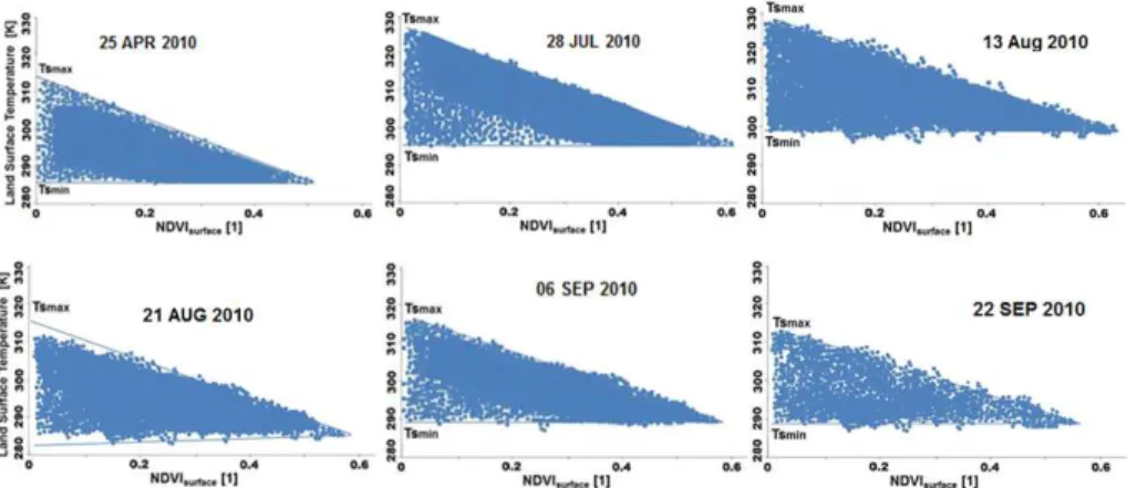
stomatal transpiration of the vegetation and lower thermal inertia within the vegetation (Lambin and Ehrlich, 1996; Sandholt et al., 2002). Therefore,Tsis dependent on both, the thermal inertia and the available moisture of vegetation. This relation is ideally rep-resented in a triangle shape, when NDVIsurf data are plotted vs. correspondingTsdata (see Fig. 3). The lower line which envelopes the triangle shaped scatter plot
repre-10
sents the so-called “wet edge”, while the upper, negatively sloped line represents the so-called “dry edge” of any given (Ts; NDVIsurface)-data set.
Zeng et al. (2004) applied this method successfully to arid areas and showed that both linear relationships between Ts and NDVIsurface along the dry edge (dry border) and wet edge (wet border) assured that soil moisture could be estimated from aTs
-15
NDVIsurface scatter plot (Fig. 3). They defined a soil moisture index (SMI) for the Ts -NDVIsurface space, whose value is zero along the “dry edge” and equal unity along the “wet edge”. The line from point “A” to “C” in Fig. 3 represents the dry edge (dry border) of respective vegetated areas, while the line from point “B” to “C” indicates its wet edge (wet border). According to Zeng et al. (2004), the desired SMI value reads as follows:
20
SMI= Ts max−Ts Ts max−T
s min
(11)
where Ts max and Ts min are the maximum and minimum surface temperatures in the scatter space for a given pixel, and Ts is the remotely sensed surface temperature at a given pixel for a given NDVIsurf. According to Eq. (11) SMI is the ratio of two temperature differences (for a given pixel); for instance, the value of (Ts max−Ts) at
25
ACPD
15, 34533–34604, 2015Contribution of soil biogenic NO emissions during
growing season
B. Mamtimin et al.
Title Page
Abstract Introduction
Conclusions References
Tables Figures
◭ ◮
◭ ◮
Back Close
Full Screen / Esc
Printer-friendly Version Interactive Discussion
Discussion
P
a
per
|
Discussion
P
a
per
|
Discussion
P
a
per
|
Discussion
P
a
per
|
Ts maxand Ts min are defined as linear functions of NDVIsurface and represent the en-veloping lines at the dry border and wet border of theTs−NDVIsurface scatter space:
Ts max=a1NDVIsurf+b1 (12a)
Ts min=a2NDVIsurf+b2 (12b)
where a1, a2, b1, and b2 were obtained by linear regression of known remotely
5
sensed data along the dry and wet edges. The SMI value for a given data point “D” (NDVIsurface,D; Ts,D) is calculated from Eq. (11) using Eqs. (12a) and (12b) to obtain Ts max, D andTs min, D.
2.4.5 Calibration of satellite derived SMI data
The basic concept to convert satellite derived dimensionless SMI data into the
vol-10
umetric soil moisture content (θv) is discussed by Wagner et al. (1999) and Mallick et al. (2009). For that, specific and characteristic soil moisture values for soils of each considered land use type are needed, preferably those which may correspond to the lower and upper limits of (dimensionless) SMI data (0 and 1, see Sect. 2.4.4). As a first approximation one may assume as the lower limit for agriculturally managed land use
15
types the volumetric soil moisture content at permanent wilting conditions (“permanent wilting point”, PWP). The PWP is defined as the level at which plants will irreversible, if additional water is not provided; to avoid this the plants have to be irrigated before the PWP is reached. After heavy rain events and after irrigation events soils of vegetated land use types may reach the status of so-called (over) saturation (flooding irrigation
20
equals to about 10–15 cm H2O column on the soil); however, this status is only ob-served for about 12–24 h, after the field capacity (FC) is equilibrating. Therefore, the soil specific value at conditions of FC may be used as upper limit for the volumetric soil moisture content. Soil specific data of PWP and FC (or for flooding irrigation multiples of FC) are typically used in irrigation scheduling, calculation of plant available water,
25
ACPD
15, 34533–34604, 2015Contribution of soil biogenic NO emissions during
growing season
B. Mamtimin et al.
Title Page
Abstract Introduction
Conclusions References
Tables Figures
◭ ◮
◭ ◮
Back Close
Full Screen / Esc
Printer-friendly Version Interactive Discussion
Discussion
P
a
per
|
Discussion
P
a
per
|
Discussion
P
a
per
|
Discussion
P
a
per
|
of volumetric soil moisture content,θv, min at PWP andθv, max at FC, are usually deter-mined by standardized laboratory measurements of water tension (pF) on undisturbed soil samples (θv maxat pF=1.8;θv, minat pF=4.2). By knowing the corresponding bulk soil densities, volumetric soil moisture contents (θv, min and θv, max) can be converted to gravimetric soil moisture contents (θg, minandθg, max). Withθg, minandθg, max of soil
5
samples from each considered land use type, the corresponding SMI data (dimen-sionless; ranging from 0 to 1) can be transformed to data of gravimetric soil moisture content (θg) by:
θg=θg, min+SMI(θg, max−θg, min) (13)
which means SMI=1 atθg, maxand SMI=0 atθg, min.
10
For non-vegetated arid and hyper-arid soils (desert), the lower limit of the volumetric soil moisture content is certainly (much) lower than that at the PWP and the upper limit (at FC) may be reached at best a few hours (days) per year. Therefore, in the case of bare and desert soils, we decided to use for the lower limit a value which corresponds to “residual water” of the desiccated soil sample measured by dry mass determination
15
as gravimetrical soil moisture after stopping each incubation experiment in the lab. Unfortunately, laboratory measurements of water tension have not been performed on the soil samples from the Tohsun oasis (desert, cotton and grape fields). Land use type specific data forθg, minandθg, max have been substituted by averages of water tension measurements (at pF=1.8, 4.2, 6.8) performed on undisturbed soil samples taken
20
around the Taklimakan desert during 2010 (Behrendt et al., 2014): at 8 desert sites (around the oases of Awati, Kuche, Milan, Mingfeng, Qiemo, Ruoqiang, Sache, and Waxxari), at 7 cotton field sites (within the oases of Awati, Kuche, Milan, Qiemo, Sache, Waxxari), and at 3 jujube plantation sites (within the oases of Milan, Minfeng, Qiemo); grapes and jujube both of them belong to the bushy agricultural landscape type and
25
ACPD
15, 34533–34604, 2015Contribution of soil biogenic NO emissions during
growing season
B. Mamtimin et al.
Title Page
Abstract Introduction
Conclusions References
Tables Figures
◭ ◮
◭ ◮
Back Close
Full Screen / Esc
Printer-friendly Version Interactive Discussion
Discussion
P
a
per
|
Discussion
P
a
per
|
Discussion
P
a
per
|
Discussion
P
a
per
|
and jujube. During July–September 2010, soil sensors (MSR® 165 data logger; see Sect. 2.2) have been buried at 2.5 cm depth at the site of Tohsun County Meteorological Station (bare soil), while in irrigated cotton, and jujube fields of the oases of Kuche and Minfeng the Frequency Domain Reflectometry (FDR) probes (ECHO-5, Decagon, USA) were used. Following the measurements of soil moisture (5 min resolution) of the
5
latter two sites, we found, due to the applied irrigation schedules, that the lower limit of θg (θg, min) was never as low as that of the PWP, i.e. regular irrigation always started long before unwanted permanent wilting conditions were reached. Instead, temporal variation of the gravimetric soil moisture content was observed between upper limits θg, max, jujube at 1.5 × FC and θg, max, cotton at 1.75 × FC (equilibrating at the time of
10
(flooding) irrigation),θgat FC (equilibrating about 2.5–3.5 days after stop of irrigation), and lower limitsθg, min, jujubeat 0.25×FC andθg, min, cotton at 0.5×FC (after about 14 days, and shortly before the next irrigation cycle). We adapted these findings for the cotton and grape fields of the Tohsun oasis. Finally, we used the followingθg, min and θg, maxvalues for soil originating of the three land use types of Tohsun oasis: 0.167 and
15
0.586 for cotton soils, 0.086 and 0.514 for grape soils, andθg, min=θg, max=0.0028 for desert soils.
2.4.6 Validation and calibration of satellite derived surface temperature and soil moisture data
Six Landsat images of sufficient quality were available during our observation period
20
in 2010, namely those of 25 April (10:40 LT), 28 July (10:40 LT), 13 August (10:35 LT), 21 August (10:35 LT), 6 September (10:35 LT), and 22 September (10:35 LT). Since only one soil sensor has been buried at the Tohsun oasis during this period (2.5 cm depth; “bare soil”; Tohsun County Meteorological Station), validation of satellite derived Ts (LST) and θg (SMI) data of Tohsun oasis could be realized only for the “desert”
25
ACPD
15, 34533–34604, 2015Contribution of soil biogenic NO emissions during
growing season
B. Mamtimin et al.
Title Page
Abstract Introduction
Conclusions References
Tables Figures
◭ ◮
◭ ◮
Back Close
Full Screen / Esc
Printer-friendly Version Interactive Discussion
Discussion
P
a
per
|
Discussion
P
a
per
|
Discussion
P
a
per
|
Discussion
P
a
per
|
Due to soil inertia (determined by the soil heat conductivity and capacity), any surface temperature signal needs a certain time period to propagate to deeper soil layers. From our measurements of the soil temperature profile (1, 2, 6, 10 cm depth) at the desert site of the Tohsun oasis, the time delay (surface to 2.5 cm depth) has been determined to 25 min. Consequently, for the intended validation of the satellite derived Ts (LST)
5
data, soil temperature measurements at Tohsun County Meteorological Station (5 min resolution) have been averaged (±10 min) at a center time 25 min before the overflight
of the satellite.
Behrendt et al. (unpublished data) provided the relationship between the relative humidity of soil air and the gravimetric soil water content (θg) based on laboratory
cal-10
ibration by a vapor sorption analyzer on soil samples from the Taklimakan desert. For the intended validation of satellite derivedθg (SMI) data, the soil air relative humidity measurements at the Tohsun County Meteorological Station (5 min resolution) have been averaged (±10 min) at the respective overflight time of the satellite.
2.4.7 Two dimensional soil NO emission model
15
Soil NO production and soil consumption rates, as well as the resulting net NO re-lease rates from the top soil of wheat, corn, cotton, and jujube fields of the irri-gated oasis agriculture (around the Taklimakan desert) have been characterized by Behrendt et al. (2014) and Mamtimin et al. (2015), respectively. The study by Mam-timin et al. (2015) has delivered evidence for a strong contribution of biogenic soil NO
20
emission from these managed (irrigated, fertilized) dryland soils to the local total NO2 budget. Having (a) the net potential NO flux (FNOdependent onTsandθv), (b) the sur-face soil temperatures (Ts), (c) the volumetric soil moisture contents (θv), and (d) the areal distribution of the three land use types (cotton, grapes, and desert) of the Tohsun oasis available, a 2-D NO emission model was built with Arc GIS to determine the two
25
ACPD
15, 34533–34604, 2015Contribution of soil biogenic NO emissions during
growing season
B. Mamtimin et al.
Title Page
Abstract Introduction
Conclusions References
Tables Figures
◭ ◮
◭ ◮
Back Close
Full Screen / Esc
Printer-friendly Version Interactive Discussion
Discussion
P
a
per
|
Discussion
P
a
per
|
Discussion
P
a
per
|
Discussion
P
a
per
|
To classify these field specific vegetation types, pre-processing the Landsat imagery and image interpretation has to be performed. To effectively record the image data, histogram equalization and edge detector techniques (Jensen, 2005) were applied dur-ing image pre-processdur-ing. By usdur-ing suitable edge detectdur-ing functions, Landsat images were enhanced and boundaries between different classes were strongly highlighted
5
for effective subsequent image interpretation. Due to the significant requirements for the different areas of interests (AOIs) of image classification, in-situ GPS data (160 points) from the field campaigns (2010) and also from previous field investigations (2006, 2008) were used. Spectral signatures of in situ data were collected by digitizing, and were consequently used to classify all pixels. For that, image spectral analysis and
10
the mostly used supervised classification method of maximum likelihood by Jensen (2005) was performed. This procedure ensured that (a) spectral characteristics of all AOIs were used, and (b) every pixel (both, within and outside AOIs), was assessed and associated to that land-cover of which it has the highest likelihood of being a mem-ber. Then, raster data of the three most frequent land-cover types of the Tohsun oasis
15
(cotton, grapes and desert) were implemented in the 2-D soil NO emission model to quantify the NO emissions for each location. By that, the empirical relationship of soil NO emission to its driving parameters (Eq. 2) was used to up-scale the laboratory estimates into two dimensions:
FNO(x,y) = FNO θg, 0(x,y),Tsoil,0
g θg(x,y)
h(Tsoil(x,y)) (14)
20
whereFNO(x,y) is the land use type specific net potential NO fluxθg(x,y) andTsoil(x,y) are the land use type specific gravimetric soil moisture content and soil temperature at the center of each grid point (30 m×30 m),θ
g,0(x,y) is the land use type specific, so-called optimum gravimetric soil moisture content (i.e., where the maximum NO release has been observed), and Tsoil,0 is the reference temperature (here: 25
◦
C; identical
25
for all land use types). The land use type specific exponential soil temperature curve h(Tsoil(x,y)) and the land use type specific optimum soil moisture curveg θg(x,y)
ACPD
15, 34533–34604, 2015Contribution of soil biogenic NO emissions during
growing season
B. Mamtimin et al.
Title Page
Abstract Introduction
Conclusions References
Tables Figures
◭ ◮
◭ ◮
Back Close
Full Screen / Esc
Printer-friendly Version Interactive Discussion
Discussion
P
a
per
|
Discussion
P
a
per
|
Discussion
P
a
per
|
Discussion
P
a
per
|
defined by Eqs. (15) and (16):
h(Tsoil(x,y))=exp
lnQ
10,NO(x,y)
10 Tsoil(x,y)−Tsoil,0
(15)
g θg(x,y)
= θg(x,y) θ0(x,y)
!a
exp
"
−a
θg(x,y) θ0(x,y)
−1 !#
(16)
Land use type specific shape factors “a” of corresponding optimum soil moisture curves were derived from laboratory drying-out incubation studies on the
correspond-5
ing soil samples according to Behrendt et al. (2014). The land use type specific quantity Q10,NO is the (logarithmic) slope of h(Tsoil), which was also derived from the laboratory measurements; applying two different soil temperatures, Tsoil,0 and Tsoil,1 (Tsoil,1−Tsoil,0=10 K), land use type specificQ10,NOis defined by
Q10,NO =
lnFNO θg,0,Tsoil,1
−lnFNO θg,0,Tsoil,0
Tsoil,1−Tsoil,0
(17)
10
In terms of data handling, an important requirement for modelling of the 2-D NO emis-sion is the accurate description of unique identifiers. Two identifiers have been at-tributed to each grid point (x, y), namely (a) the geographic coordinate (x, y of the center of each grid point of the corresponding pixel), and (b) the object ID number followed by a description of (i) the land-use type, (ii) the land use type specific net
po-15
tential NO flux, (iii) the land use type specific gravimetric soil moisture content, and (iv) the land use type specific soil temperature. Finally, land use type specific 2-D NO emis-sions were calculated for the begin, the middle and the end of the vegetation period.
2.5 Biogenic emission from soil vs. anthropogenic emission of the Tohsun oasis
20
in-ACPD
15, 34533–34604, 2015Contribution of soil biogenic NO emissions during
growing season
B. Mamtimin et al.
Title Page
Abstract Introduction
Conclusions References
Tables Figures
◭ ◮
◭ ◮
Back Close
Full Screen / Esc
Printer-friendly Version Interactive Discussion
Discussion
P
a
per
|
Discussion
P
a
per
|
Discussion
P
a
per
|
Discussion
P
a
per
|
completeness of available data, (c) very different temporal scales of existing data, and (d) to find the common, reconciled temporal scale for the comparison. One would expect that anthropogenic emissions of the Tohsun oasis will peak during the winter months (due to domestic heating), while minimum emissions will prevail during sum-mer. In contrast, biogenic emissions will exhibit the opposite temporal pattern (due to
5
the exponential response of biogenic NO release from soils, see Sect. 2.4.7). Conse-quently, the common, reconciled temporal scale for the intended comparison should be at least seasonal, preferably monthly. However, calculating mean monthly land use type specific soil emissions from mean monthly data of soil temperature and soil mois-ture (according Eqs. 15–17) seems inappropriate due to (a) the strongly non-linear
10
response of the soil NO release from both variables, (b) large diel variations of the sur-face soil temperature (e.g. 10–60◦C; desert soil; July), and (c) large weekly variations of soil moisture caused by the applied irrigation schedules. Furthermore, fertilization application (usually concurrent with irrigation) leads to fertilizer amount and time de-pendent amplification of NO fluxes from the agriculturally managed oases soils.
Con-15
sequently, mean monthly land use type specific soil NO emissions have to be averaged from data calculated on much shorter time scales (<1 h, in detail see Sect. 2.5.2). To make soil biogenic emissions (given in terms of mass of NO and HONO, respectively) comparable to the anthropogenic ones (which have been provided in terms of NO2 only), respective numbers were multiplied by the respective ratios of corresponding
20
molecular weights (MNO2/MNO,MNO2/MHONO).
2.5.1 Annual anthropogenic NO2emission of the Tohsun oasis
Tohsun oasis’s anthropogenic NO2 emissions predominantly originate from fossil fuel combustion of the energy and traffic sectors. To quantify the amount of an emitted sub-stance from a source like fossil fuel combustion, specific emission factors have to be
25
avail-ACPD
15, 34533–34604, 2015Contribution of soil biogenic NO emissions during
growing season
B. Mamtimin et al.
Title Page
Abstract Introduction
Conclusions References
Tables Figures
◭ ◮
◭ ◮
Back Close
Full Screen / Esc
Printer-friendly Version Interactive Discussion
Discussion
P
a
per
|
Discussion
P
a
per
|
Discussion
P
a
per
|
Discussion
P
a
per
|
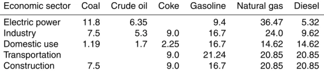
able sparsely statistical data, the most frequently used fuel types in Tohsun are coal, coke, crude oil, natural gas, diesel, and gasoline. Thus, we used those NOx emission
factors which are widely used in P.R. China (Hao et al., 2002; Zhang et al., 2009; Shi et al., 2014), and which are based on the following equation:
EiN,j(k),f(t) =1−PN
i,j(k),f(t)
·KN
i,j(k),f(t)·Fi,j(k),f(t) (18)
5
HereEN (in kg) is the mass of emitted NOx (calculated as NO2),P
N
is the dimension-less removal efficiency of the emission reduction technology (if applied);KN (in kg t−1) is the emission factor (mass of emitted NOxper mass of fuel, weighted as NO2);F (in t) is the fuel consumption; the subscript “i” represents any autonomous region or province of P.R. China (here: Turpan County); the subscript “j(k)” is the emission source
cate-10
gory in the economic sector “k”; the subscript “f” is the fuel type, and “t” is the time (year). It should be noted that information on Tohsun County’s fuel consumption is only available on an annual basis; however, coal is the dominating fuel type of energy con-sumption (65 % of total; Pu, 2009, 2011). Tohsun’s heating system changed in 2007, the former inefficient central coal fired boiler was shut down and replaced by
decen-15
tral heating systems. Most of the boilers of the central heating facilities were based on “low NO2burner technologies”, which means that the potential coefficient of emission-reduction for coal-fired thermal power is equal to 0.67 (Zhou, 2006; Mao et al., 2012). For calculation of the emission factor of electric power, we multiplied the uncontrolled emission factors by the new removal efficiency coefficient. The NO2 emission factors
20
used in this study are summarized in Table 1.
2.5.2 Specific land use type soil temperature, gravimetric soil moisture content, and fertilizer factor
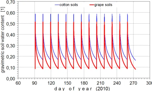
Due to the very low soil temperature before and after the growing season (see Fig. 1b), most of the soil surface is expected to be frozen andFNO from any soils of the Tohsun
25
ACPD
15, 34533–34604, 2015Contribution of soil biogenic NO emissions during
growing season
B. Mamtimin et al.
Title Page
Abstract Introduction
Conclusions References
Tables Figures
◭ ◮
◭ ◮
Back Close
Full Screen / Esc
Printer-friendly Version Interactive Discussion
Discussion
P
a
per
|
Discussion
P
a
per
|
Discussion
P
a
per
|
Discussion
P
a
per
|
the period April to September. Calculation of mean monthly land use type NO emis-sions (according Eqs. 15–17) needs temporally high resolution (<1 h) data sets of soil temperature and gravimetric soil moisture content for grape, cotton, and desert soils. In-situ measurements of both quantities (5 min resolution) at the Tohsun oasis have been performed only for the land use type “desert”, and only for the period 1 July to
5
30 September 2010 (see Sect. 2.2). During the same period, soil temperature and soil moisture (at 2.5 cm depth) have also been measured for the land use types “cotton fields” and “jujube fields” (which substitute Tohsun oasis’ grape fields; see Sect. 2.4.5) at the Taklimakan oases Kuche (41.5360◦N, 82.8546◦E) and Minfeng (37.0534◦N; 82.0760◦E), respectively. For the spatial adjustment and temporal scaling of the three
10
soil temperature data sets (“desert”, “cotton fields”, “grape fields”), the corresponding Landsat satellite derived surface temperatures of 25 April, 28 July, 13 and 21 August, and 6 and 22 September 2010 (approx. 10:45 LT) have been used (see below).
For the entire growing season (April–September 2010) a constant value of the gravi-metric soil moisture content (0.0028) has been chosen for Tohsun oasis’ desert soils.
15
Following the observations at the oases of Kuche and Minfeng, a temporally constant irrigation schedule, starting at 1 April and repeated every 2 weeks, as well as corre-sponding “drying-out” shape functions have been adapted for the land use types “grape soils” and “cotton soils” of the Tohsun oasis.
To maintain the productivity of the grape and cotton fields of the Taklimakan oases,
20
the soils regularly receive considerable N-containing fertilizer amounts (see Sect. 2.1). The impact of the fertilizer application on the NO-fluxes from arable soils of the Tak-limakan oases was recently investigated by Fechner (2014) using the laboratory dy-namic chamber system described by Behrendt et al. (2014). Dependent on the applied fertilizer amount (FA), NO-fluxes from all soil samples increased considerably,
imme-25
ACPD
15, 34533–34604, 2015Contribution of soil biogenic NO emissions during
growing season
B. Mamtimin et al.
Title Page
Abstract Introduction
Conclusions References
Tables Figures
◭ ◮
◭ ◮
Back Close
Full Screen / Esc
Printer-friendly Version Interactive Discussion
Discussion
P
a
per
|
Discussion
P
a
per
|
Discussion
P
a
per
|
Discussion
P
a
per
|
range of gravimetric soil moisture, and (b) there is an only moderate amplification of the net NO release (net NO potential flux) with soil temperature. The fertilizer effect may be considered by the multiplicative, FA-dependent, and dimensionless “fertilizer factor (FF)” applied to the standard net releaseJNO(θg,0,Tsoil,0) in Eq. (2), and as the FA-dependent, and the dimensionless “Q10 factor (Q10F)” also multiplicatively applied
5
toQ10 (the logarithmic slope of the exponential soil temperature curveh(Tsoil)). Given fertilization amounts FA=100, 200, 300, and 400 kg (N) ha−1 result in FF=142, 179, 205, and 226, andQ10F =1.21, 1.24, 1.25, and 1.26, respectively.
2.5.3 Data assimilation
Unfortunately, data of fossil fuel consumption from the different economic sectors of
10
Tohsun County (see Sect. 2.2) are only available on an annual basis. For down-scaling to mean monthly values, the corresponding mean monthly percentage of NO2 of Urumqi (140 km NNW of Tohsun) has been used. Based on the data from Mamtimin et al. (2011) the monthly percentage of NO2for Tohsun adapted from Urumqi and ex-pressed as following: 0.148, 0.157, 0.125, 0.069, 0.041, 0.035, 0.031, 0.046, 0.051,
15
0.066, 0.099, and 0.132 for January to December, respectively.
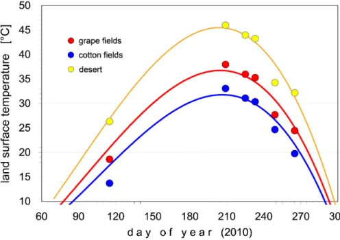
For temporal up-scaling of the Landsat satellite derived land use type specific surface temperature data, corresponding values for “desert”, “cotton fields”, “grape fields” have been fitted by 3rd order polynomials with respect to the day of year (DOY) 2010 (see Fig. 4). As a result, land surface temperatures (at 10:45 LT; i.e. satellite overflight) for
20
the Tohsun oasis’ land use types can be calculated for every individual day between 1 April and 30 September 2010. Soil temperature measurements (5 min) for the land use types “desert”, “cotton fields”, and “grape fields” are available only for the period 1 July to 30 September 2010. To obtain data sets suitable for the entire considered time period (April–September 2010), the following approach has been chosen. Each data
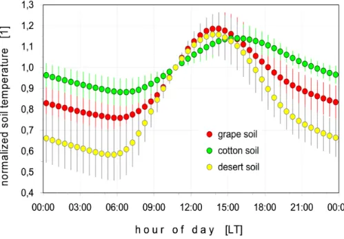
25
point of a particular day has been normalized by the mean value observed at 10:45 LT (±15 min), the time of the Landsat satellite overflight. A data set of mean diel variation