1INSA de Lyon, L.G.C.I.E. – Laboratoire de G´enie Civil en Ing´eni´erie Environnementale, 69100, Villeurbanne cedex, France 2Cemagref of Grenoble, Snow Avalanche Engineering and Torrent Control research unit, BP 76, St Martin d’H`eres, France Received: 8 March 2010 – Revised: 28 May 2010 – Accepted: 18 June 2010 – Published: 15 July 2010
Abstract. This paper deals with the assessment of phys-ical vulnerability of civil engineering structures to snow avalanche loadings. In this case, the vulnerability of the el-ement at risk is defined by its damage level expressed on a scale from 0 (no damage) to 1 (total destruction). The vul-nerability of a building depends on its structure and flow fea-tures (geometry, mechanical properties, type of avalanche, topography, etc.). This makes it difficult to obtain vulnerabil-ity relations. Most existing vulnerabilvulnerabil-ity relations have been built from field observations. This approach suffers from the scarcity of well documented events. Moreover, the back analysis is based on both rough descriptions of the avalanche and the structure. To overcome this problem, numerical sim-ulations of reinforced concrete structures loaded by snow avalanches are carried out. Numerical simulations allow to study, in controlled conditions, the structure behavior under snow avalanche loading. The structure is modeled in 3-D by the finite element method (FEM). The elasto-plasticity framework is used to represent the mechanical behavior of both materials (concrete and steel bars) and the transient fea-ture of the avalanche loading is taken into account in the simulation. Considering a reference structure, several sim-ulation campaigns are conducted in order to assess its snow avalanches vulnerability. Thus, a damage index is defined and is based on global and local parameters of the structure. The influence of the geometrical features of the structure, the compressive strength of the concrete, the density of steel in-side the composite material and the maximum impact pres-sure on the damage index are studied and analyzed. These simulations allow establishing the vulnerability as a function of the impact pressure and the structure features. The de-rived vulnerability functions could be used for risk analysis in a snow avalanche context.
Correspondence to:D. Bertrand ([email protected])
1 Introduction
The recent economic and social development of mountain-ous regions needs the extension of occupied areas. The topo-graphy configuration is favorable for natural hazards such as rock falls, debris flows and snow avalanches. The scarceness of the safe areas makes it difficult for the decision maker to reconcile security and development. To protect inhabitants against the natural threats, new strategies for risk mitiga-tion have to be adopted (for instance Barbolini and Keylock, 2002; Fuchs et al., 2005; Grˆet-Regamey and Straub, 2006). Quantitative risk analysis, which expresses the risk as func-tion of the hazard (A) and the vulnerability of the element at risk (V), is one of the main steps.
Currently, the assessment of the vulnerability of civil engi-neering structures is still difficult even if the back-analysis of observed events allowed establishing vulnerability relations of a structure damaged by a snow avalanche (Jonasson et al., 1999; Keylock and Barbolini, 2001; Barbolini et al., 2004a; Cappabianca et al., 2008). However, only a few well doc-umented events are available and the uncertainty of the ob-tained relations is very high (see for example Bell and Glade, 2004). The weaknesses of these approaches induce a rough evaluation of the risk even if the hazard is well quantified (Eckert et al., 2008).
This is the reason why a new approach based on numer-ical simulations of structures submitted to snow avalanche loadings is developed in this paper. This approach allows to solve solving complex mechanical problems involving non-linear behaviors of materials in dynamic conditions. These results make it possible to get data required to build physical vulnerability relations.
the avalanche magnitude and the damage level of the struc-ture can be derived. The main interest of numerical sim-ulations to explore the structure behavior in order to accu-rately control the parameters involved in the system (geome-try, loading, materials, etc.).
In this paper, the attention is focused on reinforced con-crete structures. The specific pressure field caused by an avalanche is described and its analytic modeling is presented. Next, the constitutive model of the building material is ex-posed. After, a damage index is proex-posed. The definition of the latter is based on the maximum displacement of the structure, the number of cracks and the yielding inside the concrete or the maximum yield strains into the steel bars re-maining after the loading. All these quantities are deduced from the FEM simulation campaigns. Finally, these results are used to derive vulnerability relations according to the structure and the traits of the avalanche.
2 Vulnerability context
The vulnerability of an entity (for instance an organization, a geographical zone, etc.) is itsweaknessfor a given event. As a general rule, the entity belongs to one of the four following classes: human, technical, information and financial. The occurrence of the event, often random, generates the partial or total destruction of the entity. Related to the four previ-ous classes, consequences of the event can be expressed in terms of human life losses, physical and technical damages, information losses, damage to the partnerships, and losses of income. From this point of view, this definition of the term
vulnerability is very general and has several meanings de-pending on the context and entity considered. In this paper, the term vulnerability refers to the physical damage of struc-tures subjected to a snow avalanche.
In this context, few definitions have been proposed. Wil-helm (1998) has proposed vulnerability relations for five dif-ferent buildings classes (light construction, mixed construc-tion, masonry, concrete buildings and reinforced buildings). The damage potential, that is to say the vulnerability, is ex-pressed as a function of the avalanche pressure. However, as highlighted by Wilhelm (1998), thresholds related to the structure strength limits are only introduced to assess the pos-sible extent of damage. The values of these parameters are chosen from an average point of view and thus the proposed vulnerability relations are quite approximate.
Jonasson et al. (1999) has proposed some vulnerability relations linking the probability to survive inside a build-ing when an avalanche of known velocity hits it. The latter relations have been calibrated from catastrophic avalanche events at Sudavik and Flateyri (Iceland). Afterwards, Bar-bolini et al. (2004b) revisited the same data set and proposed a new vulnerability relation accounting for the influence of the construction technology on the building resistance.
According to IUGS (1997) and Barbolini et al. (2004b), a definition of the risk for settlements exposed to snow avalanches can be written as follows:
R(Ta, Ts, Ps)= Z +∞
0
pA(Ta, Ia)·V(Ts, Ps, Ia)dIa (1) whereTais the type of the avalancheA(dense, powder or mixed). pA(Ta, Ia)is the probability density function. The latter is the derivative function of the probability that the avalancheA(of typeTa) reaches or exceedsIawhereIa rep-resents the intensity of the avalanche. The hazard predeter-mination allows relating the exceedance probability to the intensity. V(Ts, Ps, Ia)is the vulnerability of the structure which has a technologyTs(e.g. reinforced conrete buildings, masonry house, steel structures, etc.), mechanical properties Ps, and which is submitted to a snow avalanche of inten-sityIa. Considering Eq. (1), many parameters are involved in this general definition. Thus, it appears difficult to de-rive such a complex equation only from such a limited set of field data. Nevertheless, the proposed methodology based on intensive use of numerical models can overcome this prob-lem by simulating the mechanical response of the structure in controlled conditions. All the variables involved in this formulation have to be defined. In this paper, the attention is focused on the vulnerability relation (V) of a specific re-inforced concrete structure and on the pressure field (P(x, z, t)) of a snow avalanche (Ta,Ia).
3 Pressure field modeling 3.1 Avalanche description
A snow avalanche is a rapid mass flow. The driving force inducing the movement is gravity. The avalanche involves a heterogeneous snow mantle made of several layers of vari-ous mechanical and geometrical properties. The mechanical strengths of the layers are strongly related to the climatic his-tory of the snow cover, to the snow masse release, and also to the avalanche path topography. The release causes are vari-ous. Stability loss can result from meteorological fluctua-tions such as a rain or a temperature increase. Snow pre-cipitation or snow drifts increase the snow weight and thus the strength limit can be exceeded. Finally, under an exter-nal load such as a skier or cornice, cohesion loss in the snow layer can appear due to ruptures in the snow and lead to an avalanche.
Fig. 1.Schematization of a multi-layer avalanche.
the flow, a suspension of snow particles develops and induces the formation of a cloud. The heigth of the cloud can reach one hundred meters.
Huge avalanches are composed of several layers of snow featured by different velocities and densities. These latter are themixedavalanches. The lower part develops a dense flow whereas the higher part is a powder cloud of snow (Fig. 1). These phases influence the pressure distribution applied to the obstacle (Norem, 1991).
3.2 Pressure of an avalanche
During the fifties, the study of the impact of an avalanche on obstacles was undertaken by Voellmy (1955). Since this study, several field or laboratory experiments have been con-ducted (Kotlyakov et al., 1977; Eybert-Berart et al., 1978; Shurova and Yakinmov, 1993; Berthet-Rambaud, 2007). The pressure measurements showed a high spatio-temporal vari-ation and no study has been exhaustive enough to fully quan-tify the impact pressure from the dynamic flow parameters.
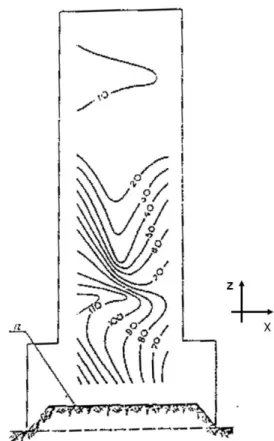
For instance, the in situ experimental results of Kotlyakov et al. (1977) carried out at a real scale (Fig. 2) give the space distribution of maximum pressure applied to a flat obstacle perpendicular to the flow. These results develop a strong heterogeneity from one experiment to another. The spatio temporal pressure distribution depends on several parame-ters such as the type of snow avalanche (dense or powder avalanche, dry or wet conditions, etc.) and the size and ge-ometry of the flow and the obstacle.
As a rule, in the engineering field, the pressure developed by an avalanche on an obstacle is estimated from the density (ρ) and velocity (v) using hydrodynamic analogy. The ave-rage pressure applied to the structure is defined as follows: Pav=C
1 2ρv
2
(2) whereCis the drag force coefficient (see for instance Salm et al., 1990). It depends on several variables such as the obstacle geometry and probably on the flow types. During the flowing, when the inertia dominates the rheology effects,
Fig. 2.Spatial distribution of the maximum pressure reached during the snow flow (in kPa) upon a flat surface of 8×3 m2. Experimental measurements carried out by Kotlyakov et al. (1977) on real scale test site.
the moving snow can be considered as a perfect fluid. In this case, the drag force coefficient is constant and depends only on the obstacle geometrical characteristics. In the opposite case, the rheology plays an important role, especially when close to the rest. Snow tends to behave as a yield stress fluid and can develop a solid behavior for extreme cases. There-fore,C depends also on snow properties which control the snow flow. Experimentally, Norem (1995) and Perrin (2006) have observed that pressures larger than those predicted by the hydrodynamic model can develop for low velocity of flowing. Thus, the snow avalanche pressure depends on the amount of potential flowing snow, the obstacle geometry, as well as the flowing properties (inertial or gravitational) which are related to snow properties.
3.3 Pressure field modeling
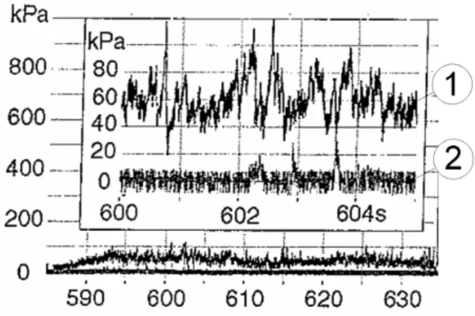
Fig. 3.Time evolution of two pressure sensors lying at 0.9 m (plot 1) and 2.1 m (plot 2) above the snow cover level (Schaer and Issler, 2001).
Previous experimental field measurements show that the pressure variations are significant during the interaction. In the case of the powder avalanches, strong fluctuations of pressure according to time are observed for in situ measure-ments at real scale (Norem, 1995; Schaer and Issler, 2001 Fig. 3 and Rammer, 2001). Similar tendencies are also ob-served in the case of dense avalanche (Eybert-Berart et al., 1977). Berthet-Rambaud (2004) carried out measurements based on the strain analysis of macro-sensors made from metal beams. Loaded by a dense snow flow, the temporal signal of the strain beam was very disturbed especially dur-ing the phase close to the front impact. In both cases, the maximum values of pressure can reach twice to three times the hydrodynamic pressure (Eq. 2).
Moreover, Kotlyakov et al. (1977) studies show the vari-ability of the maximum pressure distribution (Fig. 2) but until now the existing full scale experiments did not allow defini-tive conclusions about the spatial distribution of the snow pressure applied to an obstacle.
In the case of a dense avalanche, the vertical profile of the velocity is composed of a thin highly sheared zone, covered by a wider slightly sheared zone (Dent et al., 1998; Bouchet et al., 2004). Usually, the density is supposed constant inside the dense flow which leads to a constant pressure though the depth.
In a powder avalanche, the vertical stratification of density and velocity leads to a strong decrease in pressure along the depth. In the case of a mixed avalanche, the dense and pow-der parts are separated by a thin layer. Inside this layer, the pressure ranges from the pressure at the top of the dense part to the pressure at the base of the powder part. The retained profile is in accordance with the existing data (Schaer and Issler, 2001; Naaim-Bouvet, 2003; Gauer et al., 2007).
3.3.1 Spatial distribution
A tridimensional orthonormal basis is needed to define the pressure field. The direct orthonormal basis
ex,ey,ez is defined as a y axis which is along the normal direction to the surface interacting with the flow, z axis which is the upward vertical direction and lastlyex=ey∧ez.
The horizontal pressure (along x) is assumed constant and only depends on the flow height (z), i.e.P(x, z,t)=P(z,t). Even if experimental measurements seem to show an evo-lution of the pressure along the x axis (Fig. 2), too few ex-perimental data are available to propose a relevant horizontal distribution of pressure. In addition, considering a constant horizontal pressure distribution leads to higher damages on the structure. Thus, choosing a constant horizontal pressure distribution can be interpreted as a safety factor.
Concerning the pressure profile along the flow thickness (z), the definition of Norem (1991) is adopted. It describes an avalanche as the superposition of several snow layers. Norem (1991) proposes to identify three layers within a flow: the dense part is in contact with the substratum (a ground or mo-tionless snow cover), the second layer is the saltation layer (or fluidized layer) and finally the highest part is the powder layer. Each layer is characterized by a specific pressure field (Fig. 4). Therefore, three thicknesses are defined correspond-ing to dense layer (hd), fluidized layer (hf) and powder layer (hp). Three specific pressures are also defined : Pmax(t0) (resp.Pmin(t0)) is the maximum pressure (resp. minimum) of the distribution at time t0 andPint(t0)is the pressure at the base of the powder part. It is then possible to define the pressure using the following formula:
Pmin(t )=α1Pmax(t ) (3)
Pint(t )=(1−α2)Pmax(t )+α2Pmin(t ) (4) wheret is the time, α1 and α2 are the control parameters of the pressure field and are in[0,1]. P(z,t) is defined by pieces. The following expression arises:
Dense layer
∀z∈ [0, hd],∀t∈R+∗
P (z, t )=Pmax(t ) (5)
Fluidized layer
∀z∈ [hd, hd+hf],∀t∈R+∗ P (z, t )=Pint(t )−Pmax(t )
hf
z−hd !
+Pmax(t ) (6)
Powder layer
∀z∈ [hd+hf, hd+hf+hp],∀t∈R+∗ P (z, t )=Pmin(t )−Pint(t )
hp
z−(hd+hf) !
Fig. 4.Pressure distribution over flow thickness at timet0.
3.3.2 Time evolution
It is also assumed that the qualitative shape of the pressure profile remains constant during all the loading time, i.e. the relative pressure increase at point M(x, z) between two times is homogeneous over the profile. The time evolution of the pressure profile is controlled by the time evolution of the maximum pressure. Between two times t1 and t2 where t1<t2, it is possible to write∀(z,t1,t2)∈R×R+2
Pmax(t2)−Pmax(t1) Pmax(t1) =
P (z, t2)−P (z, t1) P (z, t1)
(8) where the left side of the equation represents the relative vari-ation of maximum pressure and the right one represents the relative variation related to the whole pressure field. For practical calculation reasons,t1=ǫ whereǫis strictly pos-itive and small enough, andt2=t is the current time. Thus ∀z and∀t
P (z, t )= 1+Pmax(t )P −Pmax(t=ǫ) max(t=ǫ)
!
P (z, t=ǫ) (9)
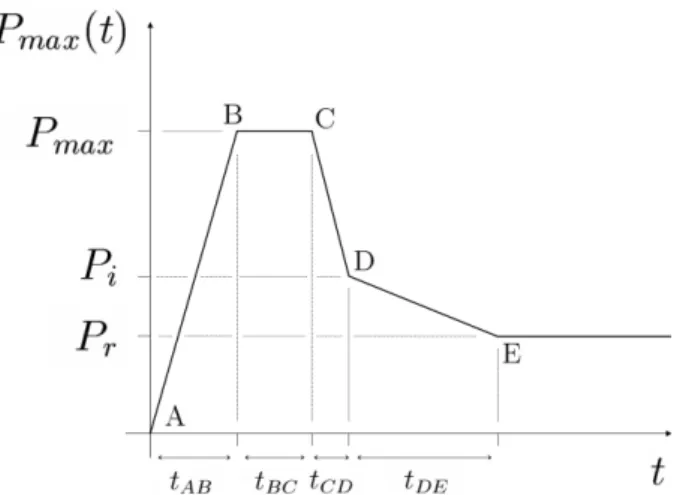
The time evolution of the maximum pressure value (Pmax(t )) applied to the structure is depicted in Fig. 5. A first linear increase of pressure from 0 toPmax(segment AB) is followed by a plateau (segment BC) of constant pressure. This profile is terminated by a progressive pressure decrease (segment CDE) until to a residual pressure (Pr).
3.4 Snow avalanche pressure field
The control parameters of the time evolution of the pressure are the maximum pressure reached during the loading phase (Pmax), the intermediate pressure (Pi), the residual pressure (Pr) and the duration of the various phases (tAB, tBC, tCD, tDE).
Fig. 5. Time evolution of the maximum pressure (Pmax(t )) of the pressure field (P(x, z,t)).
The classification is carried out from the type of avalanche (Ta) and its intensity (Ia). Firstly, it is assumed that the max-imum pressure over all the loading time (Pmax) is the main relevant feature of the avalanche intensity.
4 Structure modeling
Among all the dwelling structures found in the Alps, four main classes of buildings can be distinguished (Gr¨unthal, 1998 and Givry and Perfetini, 2006): masonries, steel struc-tures, framed buildings and reinforced concrete structures. In this paper, we focused our attention on the latter.
The shape of a civil engineering structure depends on several parameters (customer request, architect imagination, legal restrictions, standards such as EUROCODES, etc.). Whatever the shape, the building is made of three different parts: the foundation, the wall framing, and the roof. Open-ings on the building sides are potential entries for snow. This reduces the global structure strength. Thus, in several coun-tries the avalanche hazard zoning plan recommends at least to avoid openings in the wall facing the flow.
The goal of this paper is to present and apply the proposed method to a classical structure which has a simple geometry. The structure is composed of three vertical walls. The roof is not considered here.
4.1 Reinforced concrete behavior
From a rheological point of view, concrete is an isotropic material which develops a non-linear elastic behavior when the stress state reaches the elastic stress limit. Moreover, the uniaxial tensile strength of concrete is lower than its uniaxial compressive strength of an order of magnitude.
Numerical models used to describe the behavior of the concrete are numerous. At the element level, successful con-crete models have been proposed in the last decade (Bazant et al., 1996, 2000; DeBrost and Guti´errez, 1999). Nonethe-less, at the structural scale, these models often turn out to be excessively time-consuming. It is a blocking point in our objective to build vulnerability curves by the help of exten-sive numerical simulations. Consequently, a compromise be-tween simplicity and accuracy must be adopted in order to be able to represent the main degrading phenomena experienced by the composite reinforced concrete material. A classical approach for this composite material is to consider a smeared fixed crack concept for the concrete material. With this mod-eling approach, reinforcement in concrete structures is pro-vided by rebars whose nodes are the same as concrete ele-ments (perfect bond assumption) and effects associated with the rebar-concrete interface (bond slip, dowel action) are ap-proximately taken into account by introducing sometension stiffeninginto the concrete modeling.
A concrete model based on the smeared fixed crack ap-proach has been chosen. This model has been extensively used in the last decade for specimens and real civil engi-neering structures submitted to seismic loading (Ile and Rey-nouard, 2000). For instance, in the framework of U-shaped walls subjected to biaxial cyclic lateral loading, valuable re-sults have been provided enabling a feedback to the design of such structure (Ile and Reynouard, 2005). In the follow-ing the key points of this model have been presented. More details about the smeared fixed crack model adopted can be found in the previous references.
For multi-layer shell element, the plane stress assumption is made for each layer. The model is based on the plasticity theory in its uncracked state with an isotropic hardening and associate flow rule. The crack detection surface in tension follows a Nadaicriterium (ofDrucker-Pragertype) and is expressed in terms of octaedral stresses:
fcrack(σoct,τoct)=
(τoct+cσoct)
d −σ
c
b (10)
withσbcthe concrete compressive strength and where octae-dral stresses can be defined as a function of the first stress invariant I1 and the second deviatoric stress invariant J2: σoct=I31 andτoct=
q 2J2
3 .
Constant parameterscanddare given below: c=√21−α
1+α and d= 2√2
3 α
1+α (11)
withαa parameter equal to the ratio between uniaxial tensile strength (σbt) with uniaxial compressive strength (σbc). The adopted value is equal to 0.08.
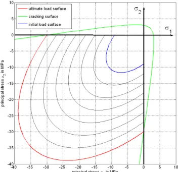
Fig. 6.Crack surface (tensile regime) and yield surfaces (compres-sive regime) depicted in principal stress space.
In compression, load surfaces are of the same type. The expression of the initial and ultimate yield surfaces in com-pression are given below:
fyield(σoct,τoct)=
(τoct+a σoct)
b −θfc (12)
where constant parametersaandbare:
a=√2 β−1
2β−1 and b= √
2 3
β
2β−1 (13)
withβparameter equal to the ratio between biaxial compres-sive strength with uniaxial comprescompres-sive strength (σbc). The adopted value is equal to 1.16.
Theθparameter indicates the initial or ultimate yield sur-face withθ=0.3 in the case of the initial load surface and θ=1 in the case of the ultimate load surface. The evo-lution of the initial yield surface to the ultimate yield sur-face in compression follows a positive isotropic hardening. A softening regime occurs with a negative isotropic harden-ing when reachharden-ing the ultimate yield surface in compression. This elasto-plastic behavior depicts the concrete behavior in its uncracked state. The crack detection surface as well as the initial and ultimate yield surfaces are shown in Fig. 6 in the principal stress space.
The crack state of the concrete model is initiated when the crack detection surface is reached in tension: avirtual crack
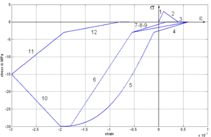
Fig. 7.Uniaxial behavior at the crack level. Thestress-straincurve is plotted in the crack referential.
first one. Cracks are irrecoverable: they remain for the rest of calculation. After the first cracking, each direction (nor-mal and parallel to the virtual crack) is then processed inde-pendently by a cyclic uniaxial law. The stress tensor in plane stress assumption is completed by the shear stress, elastically computed with a reduced shear modulusµG. µis the clas-sical shear retention factor, which satisfies 0<µ<1, and is expressed as a function of the crack opening strain account-ing for the loss of shear transfer capability at the crack level. The behavior of a point initially in tension under cyclic load-ing is depicted in Fig. 7. A similar law has been proposed when the point is initially in compression. These uniaxial laws are of phenomenological type. The behavior of a Gauss point initially in tension illustrated in Fig. 7 is commented in the following. The first path (stage 1) corresponds to the un-cracked state until it reaches the cracking surface. Afterward the concrete cracks with a negative stiffness (stage 2) and then opens with a zero stress (stage 3). When the load direc-tion changes, an increasing compressive stress is required to progressively close the crack (stage 4), followed by the non linear compressive law (stage 5). Under a new reversal load, the concrete is unloaded according to a straight line (stage 6). Stages 7–9 describe the reopening and reclosing of the crack. Stages 10–12 show the softening regime in compression after the post-peak point and a new unloading from the non linear compressive curve.
The concrete model parameters are given in Table 1. Young’s modulus and Poisson’s ratio are equal to 25 000 MPa and 0.2. Compressive and tensile strengths are taken as equal to classical values for moderate quality of concrete: 30 MPa and 2.4 MPa, respectively. The tension stiffening effect (steel and concrete interface at the crack level) is related to the zero-stress strain in tension (the end of stage 2 in Fig. 7) cor-responding to the specification of the softening behavior after cracking. In cases with little reinforcement, it is well known that this specification often introduces a mesh sensitivity in
Fig. 8.Stress-Strainrelation describing the work-hardening into the reinforcements.
the analysis: finite element predictions do not converge to a unique solution as the mesh is refined because mesh refine-ment leads to a narrower crack band. In our study, steels have been distributed uniformly across the concrete section so as to reduce this mesh sensitivity. A reasonable choice for this tension-stiffening parameter in the case of a relatively heav-ily reinforced concrete structure is to assume that the strain softening after cracking reduces the stress to zero at a to-tal strain of 10 times the strain at the cracking initiation. In addition, it is important to note that more tension stiffening makes it easier to obtain numerical solutions with respect to the convergence time-integration algorithm. With the param-eters adopted in Table 1 (tensile strength and Young mod-ulus), the zero-stress strain in tension (ǫbt) is thus equal to 10−3. The compressive ultimate strain (ǫcb) is taken as equal to 8.10−3. In order to account for the shear transfer degra-dation, the shear retention factor is initially equal to 0.4 at the cracking time then decreases to zero as a function of the normal opening strain.
The behaviour of the steel reinforcement is modeled in the classical framework of elasto-plasticity. The material is supposed isotropic and thus develops a symetrical mechan-ical response in tension and compression. The elastic do-main is characterized by Young’s Modulus and Poisson’s ra-tio. When yielding occurs, the positive work hardening of the metal is describe by astress-strain relation depicted in Fig. 8.
Fig. 9.Steel bar modeling.
4.2 Numerical modeling
The modeling of reinforced concrete structures is carried out with a tridimensional numerical model based on continuum mechanics theory. The momentum conservation Eqs. (14) and the constitutive Eqs. (15) govern the spatio temporal evo-lution of the system.
ρ∂u˙i ∂t =
∂σij ∂xj +
ρbi (14)
ˇ σ
ij=Hij σij, ξij, κ
(15) ui is the i-th component of displacement,ρis the density,bi is the i-th component of body forces,Hij is the behavior law of the material,κis the work hardening parameter of the ma-terial,ξijis the strain rate tensor and[ ˇσ]ijis the co-rotational stress tensor. These latter equations are solved through space by a finite element method (FEM). The time integration of the equations is carried out by a classical mean acceleration scheme. The problem can be written in the FEM framework as
Mx(t )¨ +Cx(t )˙ +Kx(t )=F(t ) (16) whereMis the mass matrix,Cis the damping matrix build as C=αM+βKwhereαandβ are the Rayleigh coefficients defined in the following. Fis the loading imposed on the structure. x(t )and it derivatives with respect to time (x(t )¨ andx(t )˙ ) are respectively the displacements, the velocities and the accelerations of the nodes of the FEM model.
The software CASTEM, developed by the CEA-Saclay (Millard, 1993), is used. The continuous material is re-placed by a discrete equivalent medium composed of finite
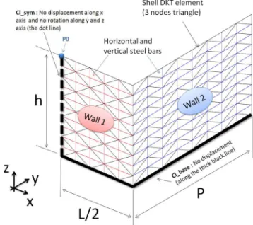
Fig. 10.FEM model of the reference structure.
elements. To model the concrete, a multi-layer thin shell rep-resentation has been adopted. The concrete walls are mod-eled by a layered thin shell Discrete Kirchoff Triangle (DKT shells – three nodes triangle) which allow reducing the num-ber of degrees of freedom by integrating the solution through the thickness of the shell. Five concrete layers with the same thickness have been considered in order to account for the flexural effects due to an out-of-plane loading.
In the case of steel bars, unidimensional elements have been used. The bar elements are two-node segments. Ver-tical and horizontal bars have been considered and for each walls, two layers of bars are modeled. The relative eccentring of the steel bars from the mid-plane of the shell is considered and thus allows describing the flexural effects (cf. Fig. 9). A perfect adhesion has been adopted between the concrete and the steel. Figure 10 represents the FEM model of the struc-ture.
Moreover, to handle the transient characteristic of the loading signal and the dynamical behavior of the system, the mass matrix and the damping matrix of the whole system are considered. Thus, the equilibrium Eq. (16) is solved by an implicit numerical scheme through the time (Newmark mean acceleration scheme).
4.3 Geometry and mechanical properties
Poisson’s ratio νb 0.2
Compressive strength σbc 30 MPa Tensile strength σbt 2.4 MPa Zero-stress strain in tension ǫbt 10−3 Ultimate compressive strains ǫbc 8.10−3
STEEL
Density ρa 7500 kg/m3
Young modulus Ea 200 000 MPa
Poisson’s ratio νa 0.3
Steel density inside the concrete γaB 0.4%
Max. elastic stress σa 500 MPa
Because many simulations have to be done to obtain vul-nerability relations, minimizing the computing time is re-quired. The geometrical symmetry of the structure and also the pressure field symmetry only allow considering half of the structure model and then allow dividing the computing time by two. Thus, on the symmetry plane, displacements along the x axis are not allowed.
Because it is an implicit resolution, the numerical scheme is unconditionally stable. Nevertheless, the timestep is cho-sen as small as it needed to describe the phenomenology in-volved during the interaction between the structure and the snow avalanche. In this case, the timestep is 10−3s and the total physical duration of the simulation is 100 s.
The parameters describing the mechanical behavior of the concrete are fixed to average usual values. All the parameters are given in Table 1.
The pressure field is applied to the upstream face of the structure defined by the x0z plan (unit normal vectory) (see
Fig. 10).
5 Structural vulnerability assessment
Experimental measurements from several authors (Kotlyakov et al., 1977; Eybert-Berart et al., 1978; Norem, 1991; Berthet-Rambaud, 2004; Gauer et al., 2007) permit us to give the order of magnitude of the pressure developed by a snow avalanche. As a rule, the maximum pressure reached during the flow is always less than 1000 kPa whatever the avalanche type. Moreover, the time evolution of the pressure depends on the avalanche type as well.
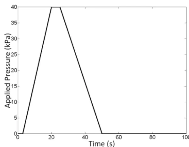
Fig. 11. Time evolution of the pressure overWall 1. Pmax corre-sponds to the maximum pressure reached (in this case 40 kPa).
Here, the chosen parameters describing the pressure dis-tribution are representative of a dense snow avalanche. The spatial distribution of the pressure field is described by a plug pressure profile. Thus, the pressure is supposed constant along the vertical direction z and the time evolution of the pressure is depicted in Fig. 11.
In order to obtain the natural frequencies of the vibration of the structure, a modal analysis is performed. First of all, this information allows knowing how the system behaves to a given loading signal. The three first natural frequencies are : f1=16 Hz,f2=30 Hz andf3=43 Hz. Thus, a characteristic time of the structure response is abouttSTR<1/16=0.0625 s. Considering the time evolution of the pressure field (the maximum pressure is reached in tCHR=17 s), it is possi-ble to assume that the loading conditions are quasi-static (tCHR>tSTR).
Secondly, due to the material behavior, a damping ratio (ξ=2%) has been taken into account. A Rayleigh damp-ing form has been chosen where the parameters α and β are involved. Usually, the calibration is based on the first two natural frequencies of the structure and can be written as : α=2ξ ω1ω2
ω1+ω2=2.622 and β=
2ξ
ω1+ω2 =1.38.10
−4 where fi=2π ωi.
Thus, the structure is loaded for a given maximum pres-sure and several strength parameters (local and global) within the structure are tracked during the simulation in order to as-sess the damage level. The latter are in our case:
– The maximum plastic strain in the steel bars (ǫa(p)). – The maximum compressive strain inside the concrete
(ǫbc(p)).
The vulnerability of the reinforced concrete structure has to be quantified from these strength parameters. The numer-ical simulations allow to know the evolution of the damages inside the concrete and the steel bars during the loading. The main problem is to adopt an adequate definition of the dam-age index.
The failure mode depends on many parameters such as the geometry, the loading conditions (pressure field, local-ized impact, imposed force or displacement), the constitutive materials, etc. Moreover, a high local damage of the structure does not necessary lead to the collapse of all of the structure elements.
At least two kinds of damage indexes can be considered and depend on the failure mode of the structure. The collapse of the building can be due to either localized damage or a uniform damage distribution.
First, when only few isolated structural elements (or ele-ment part) are involved in the failure mode of the structure, it can often be supposed that almost all the damage of the structure is due to localized degradation processes. Thus, lo-cal parameters (cracks, yielding) can be proposed for a good description of the overall structure deterioration. For in-stance, during an earthquake, reinforced concrete structures composed of vertical columns and horizontal beams or slabs would develop plastic hinges located close to the connection column/beam. In this case, high plastic strains will occur inside the concrete and inside the steel bars leading to the collapse of the structure.
On the other hand, if distributed damage inside the struc-tural elements is needed to develop the failure mode, the damage index should describe the average deterioration of the structure. Indeed, if infill walls are used to improve the strength capacity of the building, the latter will be stiffer and the damage distribution will be more uniform over all the structure. In this case reinforcements are supposed to carry additional actions coming from the external loading and also ensure good stress distribution.
For the structure considered in this paper, global damage index has been adopted. Due to the applied pressure field,
Wall 1is mainly subjected to bending andWall 2is sheared at the base. Localized zones of weakness do not exist for the structure considered. The collapse of the structure cor-responds to the initiation of a macroscopic failure dividing
Wall 1in two along the symmetry axis. The involved failure mode leads to consider a global description of the damage due to the maximum displacementδmax. ǫ
(p) a ,ǫ
c(p) b andNbc give information about the evolution of the local degradation as a function of the maximum pressure reached during the loading.
5.1 Damage index definition
The global damage index (ID) can be defined as the ratioδmaxδu whereδuis the ultimate displacement before collapse. The latter is obtained from the pushover tests. Knowingδu,ID
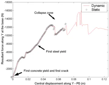
Fig. 12.Pushover test (imposed displacement) for 0.4% steel den-sity inside the concrete. Force-displacement curve obtained in quasi-static and dynamic conditions.
can be calculated fromδmaxby exploring the behavior of the structure subjected to several pressure levels. Thus, the me-chanical response of the structure to an orthogonal loading to
Wall 1is performed. In order to determineδuand to analyze the evolution of the damages when the structure is subjected to a pushover test. Two loading conditions are explored: an imposed displacement and an imposed pressure field.
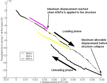
First of all, an imposed displacement loading condition has been considered. The velocity of the point P0 (along y axis) is fixed at 5 mm/s. Figure 12 depicts the degradation phases from the elastic response to the total destruction of the sys-tem. Even if loading conditions are not the same when a snow avalanche impacts the structure (force-imposed load-ing condition), in a first approximation, we assume the fail-ure modes are nearly the same (bending of the Wall 1and shearing ofWall 2). After the force peak, the structure is not able to continue resisting to the pressure. The force peak is difficult to associate with the structure collapse. Only a
collapse zonecan be identified and the determination ofδu remains tricky. This test allows to underline the development of a softening response after the maximum allowable force. In addition, Fig. 12 also compares the results of simulation in quasi-static and dynamic conditions and confirms that the response of the structure can be considered as quasi-static.
concrete) on the development of the damage is considered in-significant compared to the geometry and the strength param-eters. Thus, the elastic parameters are not considered in the vulnerability function. For the sake of simplicity, only four relevant structural parameters are taken into account in the vulnerability function derivation: the density of steel inside the concrete (γaB), the compressive strength of the concrete (σbc), the width ofWall 1(L) and its thickness (e). Finally, the vulnerability relation for the considered reinforced concrete structure can be given by:
V=V γaB,σbc, L, e, Pmax,dense avalanche (17) Sets of simulations are launched varying the maximum pressure (Pmax) applied by a given dense avalanche (plug pressure distribution) to a given structure (γaB, σbc, L and e). Pmaxis varied from 1 kPa to 200 kPa to investigate the potential damage of the structure for a wide pressure range. High levels of pressure (>200 kPa) are not explored because it is supposed that no classical structure (residential building, hotel, etc.) can resist higher pressure levels. Figure 14 de-picts the damage to the structure after the loading in terms of maximum compressive strain reached inside the concrete (ǫbc(p)) for several pressures (Pmax).
At the end of the simulations, δmax is obtained and the damage index (ID) is calculated. ID makes it possible to quantify the structure vulnerability for a given avalanche. ID=0, the structure is not damaged. The strains inside the structure remain in the elastic domain. On the other hand, ID=1 corresponds to the total destruction of the structure.
Figure 15 summarizes the various steps needed to obtain a vulnerability curve. Thus, for each vulnerability relation, a set of simulations is required which can lead to an high num-ber of simulations to perform. The influence of four param-eters is explored (γaB,σbc,Lande). For each vulnerability curve, the parameter of interest and the maximum pressure magnitude are varied and the others parameters are kept con-stant. All the vulnerability curves are plotted as contour lines of isovalues ofID(Figs. 16–19). In all the figures, the black line represents the first yield in the steel bar, the green line corresponds to the first crack inside the concrete and the red line shows the achievement of the maximum allowable com-pressive stress inside the concrete.
Fig. 13.Exemple of pushover tests for several maximum pressures. Force-displacementcurve (imposed force).
For a given loading pressure, the damage index varies sig-nificantly with the width and the thickness: the larger the width (resp. the smaller the thickness), the less the wall strength is. Indeed, for large widths of walls and small thick-nesses, the structure works mainly in bending mode. In this case, the structure collapse occurs with the break ofWall 1
(bending failure). In contrast, for small widths and large thicknesses, the structure works in shear and the maximum stress is located at the base of the walls. Thus, the failure mode could explain a significant change in the damage in-dex. In the case of concrete compressive strength, one can note that the steel contribution in the overall mechanical re-sponse of the structure is substantially always the same. The structure vulnerability reduction is mainly due to the strength increased of the cementitious matrix. The initiation of the concrete cracking and the achievement of the stress peak value (in compression) increase with the concrete strength. In contrast, the steel yield remains independent of the pres-sure applied.
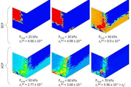
Fig. 14. Distribution of maximum compressive strain (ǫbc(p)) reached inside the concrete for several loading pressures (Pmax). BCP (resp. ACP), which meansBefore (resp. After) theCompressionPeak, describes simulations whereǫbc(p) has or not exceeded the strain value related to the maximum compressive stress inside concrete. Ifǫcbis exceeded, the concrete is highly damaged and announces the collapse of the structure.
Fig. 15. Methodology to obtain vulnerability curves for concrete structures.
Fig. 16. Vulnerability function (ID) obtained for several values of steel density (γaB).
Fig. 17. Vulnerability function (ID) obtained for several values of maximum compressive strength (σbc).
Fig. 19. Vulnerability function (ID) obtained for several values of wall thickness (e).
6 Conclusion and perspectives
This paper deals with the assessment of the physical vul-nerability of civil engineering structures submitted to snow avalanches. The structure is made of concrete and is com-posed of three vertical walls reinforced with steel bars. A methodology based on intensive use of numerical simula-tions was developed, a representative impact pressure of a dense avalanche was proposed and a damage index was de-fined as well. The latter accounts for the damage level of the structure after the avalanche. The damage index is given by the ratio between the maximum displacement reached after the avalanche loading and the maximum allowable displace-ment before the collapse of the structure.
This definition is a global definition of the damage devel-oped inside the structure, that is to say a macroscopic view of the failure. Moreover, simulations give indicators describing the state of the material on a local scale (steel yield of the bar, development of cracks, maximum compressive strains inside the concrete, etc.). These latter allow to better understand the degradation and thus the life expectancy of the structure.
From an engineering point of view, the damage index must be a scalar number in order to be easy to interpret and must be representative of all the structure mechanical behavior. The local damage indices (steel and concrete yield and con-crete crack) are generally consistent with the global indices (macroscopic displacements). The local information can be used to delineate zones of damage magnitude useful to prac-titioners.
More generally, the onset of cracks inside the concrete in-dicates the damage initiation inside this particular structure. At this stage the structure is still able to carry a relatively large load increase. In a second time, steel yield occurrence is a good indicator to identify a mechanical regime where the damage becomes particularly important. Finally, in the case of structures normally reinforced (0.2%), the imminent collapse of the structure seems to be announced when the
– Upcoming collapse: cracks, steel yield and maximum allowable compressive stress inside the concrete. The choice of the damage index remains a critical point of the approaches used to quantify structural vulnerability. From an attempt to another, risk calculation could change significantly. For instance, Barbolini et al. (2004b) used a vulnerability relation which described the probability of death for a person inside a building. They introduce in-directly the notion of human vulnerability. These relations have been obtained from deadly avalanche events in Iceland in 1995 (Jonasson et al., 1999). As noted by the authors, it seems reasonable to suppose these relations are well suited for the Icelandic housing. But these latter are fairly weak structures compared to the Alpine ones which are often build in reinforced concrete. So the used of these relations in an-other context remains questionable.
Otherwise, Wilhelm (1998) proposed a global damage in-dex relating building damage to the extent of the avalanche (AL), i.e. the estimated avalanche pressure. Five building classes are defined. In the case of reinforced concrete struc-tures, Wilhelm (1998) states that damages are observed be-tween 30 (initiation) and 40 kPa (destruction). For U-Shaped reinforced concrete structure, the same findings are observed if a structure with the following features is considered: five meters in width, a steel density of 0.2% and a compressive strength of 25 MPa. However,Wihelm’s relations seem to be established only from an expert point of view and remain a bit rough. Indeed, only the type of technology is taken into account but the type of damages is not mentioned and the structure features (geometry, material strength, etc.) are not considered.
the right choice of the damage index. Thus it is possible to propose more accurate vulnerability relations and adapt them to a given endangered zone.
Concerning the representativeness of the numerical simu-lations, it is important to notice that the frequency content of the loading signal is, for the moment, very poor. The approx-imation by a linear increase and decrease leads to suppose that the high frequencies of a real avalanche signal do not contain significant energy. Nowadays, experimental works are still in progress to measure and more accurately describe the avalanche signal in terms of energy transfer (Schaer and Issler, 2001; Thibert and Baroudi, 2010, etc.). The next step will be to load the structure with a real snow avalanche signal in order to increase the accuracy of the derived vulnerability curves. In addition, this approach can be applied to other shapes of reinforced concrete structures. Multi-stage build-ing could be considered.
On the other hand, complex structures impliy complex models which remain difficult to use because of time con-suming simulations. However, reliability approaches can bring solutions to this issue. Moreover, in the context of snow avalanches risk, the quality of these simulations could be in-creased by introducing a stochastic description of the system. Indeed, a lot of uncertainties are related to the intrinsic vari-ability of an avalanche (e.g. loading variations depending on avalanche velocity, density distribution, flow width and flow height) and to the structures features (e.g. strength variability of the reinforced concrete used for civil constructions). This is another reason why reliability approaches could be used to take into account these uncertainties into account and then obtain a hierarchy of the relevant parameters to account for the vulnerability relation derivation.
In fine, these vulnerability curves would help decision makers in the framework of avalanche risk analysis but also for the post crisis management. For instance, if the collapse of the structure did not happen, a decision has to be made after the avalanche event. Should the structure have to be destroyed or not? Is the structure rehabilitation possible? Acknowledgements. This study was supported by the European Union Project IRASMOS (Integral Risk Management of Extremely Rapid Mass Movements – Contract no.: 018412). We extend special thanks to all the members of the research group for the interest they have shown in this work.
Edited by: T. Glade
Reviewed by: S. Fuchs and another anonymous referee
References
Ancey, C.: Dynamique des avalanches, Presses polytechniques et universitaires romandes, 2006 (in French).
Barbolini, M. and Keylock, C. J.: A new method for avalanche hazard mapping using a combination of statistical and deter-ministic models, Nat. Hazards Earth Syst. Sci., 2, 239–245, doi:10.5194/nhess-2-239-2002, 2002.
Barbolini, M., Cappabianca, F., and Sailer, R.: Empirical estimate of vulnerability relations for use in snow avalanche risk assess-ment, Risk Analysis IV, Southampton, 533–542, 2004a. Barbolini, M., Cappabianca, F., and Savi, F.: Risk assessment in
avalanche-prone aeras, Ann. Glaciol., 38, 115–122, 2004b. Bazant, Z., Xiang, Y., Prat, M. A. P., and Ackers, S.: Microplane
Model for Concrete. I: Stress Boundaries and Finite Strain ; II : Data Delocalization and Verification, J. Eng. Mech.-ASCE, 122(3), 245–262, 1996.
Bazant, Z., Caner, F., Caro, I., Adley, M., and Akers, S.: Microplane Model M4 for Concrete. I: Formulation with Work-Conjugate Stress, J. Eng. Mech.-ASCE, 126(9), 944–953, 2000.
Bell, R. and Glade, T.: Quantitative risk analysis for landslides – Examples from Bldudalur, NW-Iceland, Nat. Hazards Earth Syst. Sci., 4, 117–131, doi:10.5194/nhess-4-117-2004, 2004. Berthet-Rambaud, P.: Structures rigides soumises aux avalanches
et chutes de blocs: mod´elisation du comportement m´ecanique et caract´erisation de l’interaction “ph´enomene – ouvrage”, Ph.D. thesis, Joseph Fourier University, Grenoble 1, 2004 (in French).
Berthet-Rambaud, P.: Avalanche action on rigid structures: Back-analysis of Taconnaz deflective walls’ collapse in February 1999, Cold Reg. Sci. Technol., 47, 16–31, 2007.
Bouchet, A., Naaim, M., Bellot, H., and Ousset, F.: Experimental study of dense snows avalanches: velocity profiles in steady and fully developed flows, Ann. Glaciol., 38, 30–34, 2004.
Cappabianca, F., Barbolini, M., and Natale, L.: Snow avalanche risk assessment and mapping: A new method based on a com-bination of statistical analysis, avalanche dynamics simulation and empirically-based vulnerability relations integrated in a GIS platform, Cold Reg. Sci. Technol., 54, 193-205, 2008.
DeBrost, R. and Guti´errez, M.: A unified framework for concrete damage and fracture models including size effects, International Journal of Fracture, 95, 261–277, 1999.
Dent, J., Burrell, K., Schmidt, D., Louge, M., Adams, E., and Jazbutis, T.: Density, velocity and friction measurements in a dry-snow avalanche, Ann. Glaciol., 26, 247–252, 1998. Eckert, N., Parent, E., Naaim, M., and Richard, D.: Bayesian
stochastic modelling for avalanche predetermination: from a general system framework to return period computations, Stoch. Env. Res. Risk A., 22(2), 185–206, 2008.
Eybert-Berart, A., Mura, R., Perroud, P., and Rey, L.: La dy-namiques des avalanches – R´esultats exp´erimentaux au col du Lautaret – ann´ee 1976, Communication presented to the “Soci´et´e G´eotechnique de France”, C.E.A./C.E.N.G., ANENA, Grenoble, France, 1977 (in French).
Eybert-Berart, A., Perroud, P., Brugnot, A., Mura, R., and Rey, L.: Mesures dynamiques dans l’avalanche – R´esultats exp´erimentaux du Col du Lautaret (1972–1978), in: Proceed-ings of the second international meeting on snow and avalanches, ANENA, Grenoble, France, 203–224, 1978 (in French). Fuchs, S., Keiler, M., Zischg, A., and Br¨undl, M.: The
long-term development of avalanche risk in settlements considering the temporal variability of damage potential, Nat. Hazards Earth Syst. Sci., 5, 893–901, doi:10.5194/nhess-5-893-2005, 2005. Gauer, P., Issler, D., Lied, K., Kristensen, K., Iwe, H., Lied, E.,
Ile, N. and Reynouard, J.-M.: Behaviour of U-shaped walls sub-jected to uniaxial and biaxial cyclic lateral loading, J. Earthq. Eng., 9, 67–94, 2005.
IUGS (International Union of Geological Sciences): Quantitative assessment for slopes and landslides, the state of the art, in: Landslide risk assessment, edited by: Cruden, D. and Fell, R., Proceedings of the international workshop on landslides and risk assessment, Honolulu, Hawaii, USA, 19–21 February 1997, Balkema, Rotterdam, 3–12, 1997.
Jonasson, K., Sigurosson, S., and Arnalds, P.: Estimation of avalanche risk, Reykjavik, vf-R99001-UR01, 1999.
Keylock, C. and Barbolini, M.: Snow avalanche impact pressure – vulnerability relations for use in risk assessment, Can. Geotech. J., 38, 227–238, 2001.
Kotlyakov, V., Rzhevskiy, B., and Samoylov, V.: The dynamics of avalanche in the Khibins, J. Glaciol., 19, 431–439, 1977. Mazars, J.: Application de la m´ecanique de l’endommagement au
comportement non lin´eaire et `a la rupture du b´eton de structure, Ph.D. thesis, Paris VI University, 1984 (in French).
Millard, A.: CASTEM 2000, Manuel d’utilisation, CEA-LAMBS Report, 93/007, 186 pp., 1993 (in French).
Naaim-Bouvet, F.: Approche macro-structurelle des ´ecoulements bi-phasiques turbulents de neige et leur interaction avec des ob-stacles, HDR Cemgref, 2003 (in French).
Salm, B., Burkard, A., and Gubler, A.: Berechnung von fliesslaw-inen. Eine anleitung f¨ur praktiker mit beispielen., Inst. Schnee-Lawinenforsch, Davos, 47, 37 pp., 1990 (in German).
Schaer, M. and Issler, D.: Particle densities, velocities and size dis-tributions in large avalanches from impact-sensor measurements, Ann. Glaciol., 32, 321–327, 2001.
Shurova, I. and Yakinmov, L.: Modeling the impact of snow avalanche on a structure: an experimental investigation, Izvestiya Rossiiskoi Akademii Nauk, 4, 13–17, 1993.
Thibert, E. and Baroudi, D.: Impact energy of an avalanche on a structure, Ann. Glaciol., 50(54), 45–54, 2010.
Thibert, E., Baroudi, D., Limam, A., and Berthet-Rambaud, P.: Avalanche impact pressure on an instrumented structure, Cold Reg. Sci. Technol., 54, 206–215, 2008.
Voellmy, A.: ¨Uber die Zerst¨orungskraft von Lawinen, Tech. rep., Schweiz. Bauzeitung, 73, 159–165, 212–217, 246–249, 280– 285, 1955 (in German).