Inequalities
Benoit Lorel
∗
Contents: 1. Introduction; 2. The Standard Earning Function and Empirical Implications; 3. Empirical Assessment of Brazilian Educational Inequality; 4. Look Beyond the Average and Consequences on Brazilian Wage Inequality; 5. Conclusion; A. Indicators used to quantify Education; B. Desirable Properties of the Inequality Indices; C. Tables.
Keywords:Human Capital, Education Gini, Inequality
JEL Code:C43, D63, I32, J24, O11, O15
Esse trababalho busca avaliar o grau de desigualdade educacional no Brasil baseado-se em diferentes indicatores tais como: o índice de Gini educacional, os anos médios de escolaridade e no desvio padrão educacional. Tenta-se colocar uma descrição estatistica da distribuição do capital humano no Brasil, incluindo as diferenças estaduais e regionais observadas durante a ultima metade do século. As conclusões da nossa análise são as seguintes: 1) Forte reduç ão das desigualdades educativas calculadas com o Gini edu-cacional. 2) Um retrato tripartido do Brasil parece se formar refletindo as condições iniciais. 3) Um forte aumento dos níveis de escolarização. 4) Uma relação significativa entre o Gini educacional e os anos médios de estudos. 5) O desvio padrão educacional leva aos resultados inversos do Gini educa-cional. 6) Os dados brasileiros admitem uma curva de Kuznets educacional se considerarmos o desvio padrão educacional.
This paper provides an evaluation of schooling inequality in Brazil using different indicators such as the Education Gini coefficient, the Education Stan-dard Deviation and the Average number of Years of Schooling. We draw up a statistical description of Brazilian human capital dispersion in time over the last half century, across regions and states. Our analysis suggests several con-clusions: 1) Strong reduction of educational inequalities measured by Education Gini index. 2) A three parts picture of Brazil seems to emerge, reflecting initial conditions. 3) High increase of the Average number of Years of Schooling. 4) A significant link between Education Gini and the average education length. 5) Education Standard Deviation leads to inverted results compared to Education
∗I am grateful to Universidade Santa Ursula for hospitality and to Jean Mercenier and an anonymous referee for helpful
Gini. 6) Brazilian data are consistent with an Education Kuznets curve if we consider Education Standard Deviation.
1. INTRODUCTION
As is well established,1the transmission of schooling across generations is the key channel by which
schooling inequality affects income inequality. The hope that improvements in overall access to school-ing by one generation will reduce social inequalities lies not only in the potential reductions in earnschool-ings inequality for that generation, but also in potential improvements in the distribution of education for that generation’s children. The contribution of schooling in explaining earnings inequality comes from two components - high dispersion in the distribution of schooling and large effect of schooling on earnings. Various authors have shown2that there is an important element of inertia in the evolution of schooling distributions and income distributions in developing countries. An accurate measure of the schooling dispersion within a country appears extremely useful both for positive and normative reasons. To see this, consider an asset freely traded in a perfectly competitive environment with free-entry: equalization of marginal productivities across firms will be ensured. Introduce imperfection in that market: marginal products are not equalized and an aggregation problem follows. The aggregate production function will depend not only on the average level of the asset, but also on its distribution. Because education is not perfectly tradable, the average level of schooling achievement of a country is not sufficient to reflect its human capital characteristics. We need to look beyond the average and thus have to investigate the dispersion of human capital.3 Surprisingly, at the best of our knowledge, no
such studies seem to have been made for Brazil. Our aim in this paper is to contribute to fill this gap: we provide an evaluation of schooling inequality in Brazil using different indicators such as the Educa-tion Gini Coefficient, the EducaEduca-tion Standard DeviaEduca-tion and the Average number of Years of Schooling. We are able to cartography schooling disparities, we investigate evolutions, extract some stylized facts, assess the consequences of the political reforms on education and venture some suggestions on most appropriate policies depending on regions and their development. Brazil provides us a very interesting case on more than one respect. First, its educational system has been drastically changed during the second half of the 20th century and particularly during the 90s with explicit commitment of the Brazil-ian government in providing schooling to all. Although, large efforts were effective, there still remains room for improvement on many respects:4 access to education, reception capacity in schooling and
university establishments, education quality, education equity between the various social groups and educational intergenerational mobility.5 The Brazilian case is also relevant from an economic theory
on inequalities viewpoint. Until the 1980s, Brazil had considerable success with economic growth:6its
average growth rate was of4,7%during the twentieth century (with growth concentrated in the south of the country and more particularly in regions Sul and Sudeste). Despite this remarkable performance,
1Following the Endogenous Growth Theory, we note at least 4 main reasons for a negative relation between inequality and
economic growth. 1) Increase in redistribution and fiscal pressure in line with political economics models (Benabou, 1996, Alesina and Rodrik, 1994, Alesina and Perotti, 1996, Saint-Paul and Verdier, 1993), 2) Sociopolitical tensions (Acemoglu, 1995, Benhabib and Rustichini, 1996), 3) Credit rationing (Galor and Zeira, 1993, Aghion and Bolton, 1997) and 4) Fertility (Becker and Barro, 1988, Becker et al., 1990, Galor and Moav, 2002).
2See for instance Lam (1999).
3See Appendix for a refresher on indicators proposed to quantify alternative aspects of education. 4See Barros and Mendonça (1998) concerning impact of educational reforms.
5Ferreira (2003) shows that Brazilian educational intergenerational mobility is weaker than in other developing countries and
that it differs considerably between states, between regions and between races. For instance, in region Nordeste, the probabil-ity that the son of uneducated parents remains uneducated is approximately 54%, while the same probabilprobabil-ity is ”only” 21% in region Sudeste.
social indicators in Brazil remain those of a poor country actually doing worse in terms of income in-equality than most developing countries.7 In addition, Bowman (1997) shows that a continuous rise
of income inequality occurred in Brazil despite of the increasing income per capita above the Kuznets inflection threshold of $1200 usually observed.
How does Brazil generate such extreme income inequalities, among the highest in the world? Does current patterns of educational inequalities tell us anything about the prospects for reducing inequali-ties in future generations? We shall try to provide some elements of response to these questions in this paper.
The paper is organized as follows. Section two establishes the importance of education in Brazilian wage dermination and provides a brief presentation of our methodology. In the third section, we evaluate spatial and temporal Brazilian educational inequality. Section four establishes links between indicators and implications of education inequelities on earnings inequalities. A fifth section concludes.
2. THE STANDARD EARNING FUNCTION AND EMPIRICAL IMPLICATIONS
2.1. Education as a Wage Determination Factor in Brazil
The link between education and the distribution of income has been a fundamental building block of economics of inequality.8 Theoretical models and extensive empirical evidence highlight the role
of schooling explaining the distribution of income. Our analysis below will focus on inequality in individual labor earnings, for which the importance of schooling should be more easily observed.
A useful frame of reference is the standard human capital earnings equation. Leaving experience and other factors aside, the logarithm of individuali’s labor earning can be expressed as:
log yi=α+βei+ui
whereyi is earning,ei the number of years of schooling, anduiis a random term uncorrelated with
schooling. To avoid pitfalls in time-series econometrics with incomplete data or unstable definition, we estimate this human capital earning equation by cross-section for the year 2000 using IBGE data.9
The data relate the education level (6 groups: from 0 to "15 years and more") with the income group (12 groups based on a minimum wage of 151R$: from 0 to "more than 30 times as minimum wage"). Note more than 60.05% of Brazilian earn less than the minimum wage and more than 64.7% have less than seven years of education.
The estimation results are presented in Table 1.10 Groupe2, with individuals having between 4 and
7 number of years of schooling, serves as reference group in this regression, so that coefficients should be interpreted measuring the differential return to education to that group. We see that education alone explains 87.8% of wages for the country as a whole, with the lowestR-square is quite low for region Sul, where it is yet as high as 69.9%. In a nutshell, this regression expresses forcefully the strong link that exists between education and wage earnings and justifies the current empirical assessment of the performances in term of education progress.
2.2. Earning Inequality and Education Inequality
The influence of educational inequalities and income inequalities, from standard earnings equation, the variance of log earnings,V(log y), a standard mean-invariant measure of earnings inequality, is:
7See Barros et al. (2002) for impact of an additional year of schooling on income per capita growth rate. 8See for instance Blom et al. (2001) for a Brazilian study.
V(log y) =β2V(e) +V(u)
This simple result demonstrates an important point about the link between schooling inequality and earnings inequality. If the relationship between schooling and earnings is log-linear as in traditional earnings equation above, then earnings inequality is a linear function of the variance in schooling. While there is intuitive appeal to the notion that a more equal distribution of schooling should reduce a more equal distribution of earnings, there is no theoretical reason to expect such a result. Indeed, variance of schooling (or the Education Standard Deviation) only measures the dispersion of schooling distribution in absolute terms. If we measure inequality in schooling by some standard mean-invariant inequality measure, for instance by the coefficient of variation, then if the increase in average number of years of schooling is greater than the increase in the education standard deviation, thus a decrease in schooling inequality is associated with increased earnings inequality. Hence, to measure the relative inequality of schooling distribution, developing an indicator for Gini Education is necessary.
2.3. The Education Gini: Measuring Inequality in the Distribution of Education
Achievements
Only few previous studies have estimated the Education Gini Index to analyze inequality of the education achievement distribution, none for Brazil to the best of our knowledge. We propose to do so, including an analysis of regions and states over the period 1950–2000.
Schooling distributions possess various characteristics which make inappropriate the use of some standard indicators. Because of these characteristics and despite its drawbacks (it does not satisfy the SI and SC conditions),11 the Gini Index singles out as the most appropriate. Indeed, it makes it
possible to draw Education Lorenz curves and the related stochastic dominance approach can then be used to compare distributions. Regarding methodology, schooling achievement is a discrete variable. Furthermore, its distribution is bounded: by a lowerbound of 0 (for people who did not go to school in their entire live) and by a maximal value close to 20 years of schooling. The Education Lorenz curve is then a series of points (corresponding to the number -or group- of years of schooling of the population). It is not necessary to evaluate a continuous line to get the Education Lorenz curve. Another main feature of the Education Lorenz curve is that it is not regular due to the presence of illiterates12 (or
people who never go to school (less than 1 year)): a part of this curve coincides also with the horizontal axis.
Depending on available data, the Gini formula could vary. In this paper, we make use of its distri-butions of population over the age of five, as provided by IBGE13Censos Demograficos. The formula we use is the following:14
Gini= 1
x
n X
i=1
i−1 X
j=0
pi|xi−xj|pj
where
- pi,pjare proportions of population respectively withiandjyears of schooling
- xi,xjare numbers of completed schooling years
11See Appendix for a refresher on desirable properties of inequality indices. 12Which makes inappropriate the use of the Theil index.
- nrepresents the number of schooling achievement levels
- x=Pn
i=0pixiis the average number of years of schooling of the population
The Education Lorenz curve is obtained as follows. The horizontal axis represents the cumulative proportion of populationQxwith less thanxyears of training:Q0=p0, corresponds to the proportion
of people with less than 1 year in school,Q1 =p0+p1is the proportion of the population with less than 2 years of schooling etc. The vertical axis refers toSx, the cumulative proportion of population
that has at least reached a specified level of education. Hence,S0=p0x0
x = 0,S1=
p0x0+p1x1
x etc.
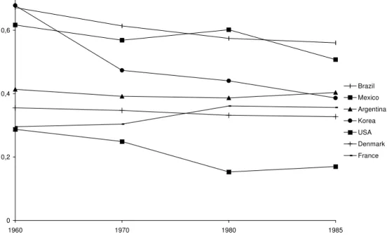
Figure 1 provides a rough international comparison15of progress achieved in terms of human capital Gini coefficient between 1960 and 1985. The panel of countries include both developed and developing countries. We first note that Education Gini in developed countries is much weaker than in developing ones. While Brazil remains in the group of highest Education Gini together with Mexico during the considered period, some countries such as Korea have remarkably managed to decrease their Education Gini. For Korea, this index was as high in the 60s as it was in Brazil, yet as low as France twenty five years later. Incidentally, observe that France and US strongly have very different trends.
Figure 1 –International Trend of Education Gini
0 0,2 0,4 0,6
1960 1970 1980 1985
Brazil
Mexico
Argentina
Korea
USA
Denmark
France
3. EMPIRICAL ASSESSMENT OF BRAZILIAN EDUCATIONAL INEQUALITY
Using the IBGE data on educational achievement for people over five,16 measured in completed
schooling year,17 we compute the Education Gini index, as well as the Average number of Years of
Schooling (AYS) and the Education Standard Deviation (ESD) for Brazil as a whole, for rural and urban, for the 5 regions (Norte, Nordeste, Sudeste, Sul and Centro-Oeste) and for the various states over the period 1950–2000. Our data set then includes 27 states with a total around 2700 observations. We can then analyze Brazilian educational inequality changes for the last half century. Among others, we find many states that in spite of having the same AYS, significantly differ in the distribution of education.
3.1. Trend of Education Gini
Using distribution of population for each education year, we estimate the Education Gini over 1950– 2000. The detailed results are reported in Table 2.18 We comment on the results and provide some
graphs.
There is a clear downward convergence between regions and states. Furthermore, the reduction of educational inequalities is impressively strong for all regions. The decline is not monotonous; how-ever, education inequality increased slightly during the 1960s.19 The first Brazilian ten-year plan for education was formulated in 1967, and it brought about a massive expansion of enrollments.
Examining the results for the country as a whole first, we observed that the Education Gini coef-ficient has sharply declined from 1950 (0,7868) to 1960 (0,6246), followed by a short increase during the 60s to reach 0,6485 in 1970 ; since the early 70s, the Education Gini has monotonically decreased reaching 0,4031 in 2000. On the whole half century, Brazilian education inequalities have decreased by 48,77%, with an acceleration during the last ten years. That decrease may be explain by various Brazil-ian education reforms. Indeed, 1971 Education Law extended the length of compulsory school from four to eight years. Moreover, the Brazilian education system has been gradually shifting the responsibility for delivering and managing education at primary level from the central government (Federal level) to the states and municipalities. 1988 Brazilian Constitution has increased the states’ and municipalities’ participation in the decision making process of educational policies.20
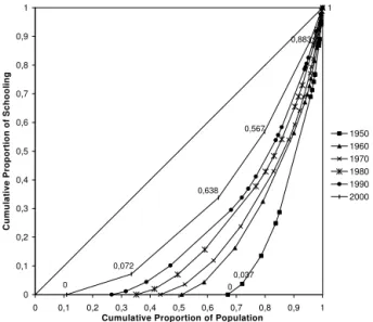
In Figure 2, we report time series of the Brazilian Education Lorenz curve. The interpretation of this graph is identical to that of the Income Lorenz curve and describes the sharing of education among population. We see that in 2000, more than10%of the population receive no education at all while
33,4%received only 7,2%of total cumulated years of schooling. In contrast in 1950, 67% of the population did not receive any education, while72%owned only3,7%of the education capital.
Despite the decentralization in the making process educational policies, the same trend can be ob-served for all regions within Brazil. Furthermore, there is a clear convergence of performance between regions, as measured by the variance of Education Gini or by the difference. It mainly occurs however, between 1990 and 2000.
As could probably be expected, Region Nordeste21remains on the whole period the region with the
highest Education Gini index, despite strong progress (particularly during the last ten years: 28,64%).
16We have used the educational information for the population aged 5 and over for emphasizing the importance of improve
in primary education access in Brazilian population, than most related studies use the information of the education for the population aged 25 years and over.
17For instance, Barro and Lee’s data set only includes the schooling level: No schooling, primary completed or uncompleted,
secondary completed or uncompleted and at least tertiary completed or uncompleted.
18See in Appendix.
19Note a different trend compared with Barro and Lee’s data, but IBGE data seem to be more complete and precise. 20See Barros and Mendonça (1997, 1998) for further details.
Figure 2 –Education Lorenz Curve – Brazil 1950–2000
1
0,037 0
0,883
0,567
0,072 0
0,638
0 0,1 0,2 0,3 0,4 0,5 0,6 0,7 0,8 0,9 1
0 0,1 0,2 0,3 0,4 0,5 0,6 0,7 0,8 0,9 1
Cumulative Proportion of Population
C
u
m
u
la
ti
v
e
P
ro
p
o
rt
io
n
o
f
S
c
h
o
o
li
n
g
1950 1960 1970 1980 1990 2000
Region Centro-Oeste (in 1950), Sudeste (in 1960) and Sul (from 1970) are the most egalitarian regions. Between 1950 and 2000, Regions Sudeste and Centro-Oeste achieved respectively the highest and the weakest progress: -51% and -43%.
Region Centro-Oeste is also the most heterogeneous region (with the highest standard deviation across Education Gini index: 0,19 in 1950 and 0,05 in 2000), while regions Sul and Sudeste are the most homogeneous (standard deviation of 0,01 for region Sul in 2000). Indeed, Region Centro-Oeste is worth noting in many respects. This Region takes advantages of the political and administrative status of Distrito Federal and State of Goias makes the most of the situation.
The Case of Goias(see Figure 3) is noteworthy. Indeed, starting from a terrible initial situation with 85,32% of the population without education in 1950, Goias expanded its basic education rapidly and eliminated illiteracy successfully and after half a century this population represent only 9,26% corresponding to the average of Centro-Oeste (9,38%).22Over decades, the Education Gini decreased by
58% (42,7% for Region Centro-Oeste and 48,77% for Brazil as a whole).
To conclude with the Education Gini index, Region Centro-Oeste contains an historical and political exception (Distrito Federal) and the development of Goias. In region Nordeste lies bad permanence feature and homogeneity, whereas Sul and Sudeste are the most homogeneous and perform the highest decreasing rate of Gini.
3.2. Dropping Out No Schooling: What remains of Educational Inequality
Previous results have documented a strong reduction of educational inequality in Brazil since 1950. However a more careful look at those results is called for: indeed, if we drop from our sample those
Figure 3 –Education Lorenz Curve – Goias – 1950–2000
0 0,1 0,2 0,3 0,4 0,5 0,6 0,7 0,8 0,9 1
0 0,1 0,2 0,3 0,4 0,5 0,6 0,7 0,8 0,9 1
Cumulative Proportion of Population
C
u
m
u
la
ti
v
e
P
ro
p
o
rt
io
n
o
f
S
c
h
o
o
li
n
g
1950 1960 1970 1980 1990 2000
members of the population that are without any education, the results, regarding the evolution of the Education Gini are extremely different, as shown by Table 3.23
No trend is apparent in the latter series, which clearly reveals that progress has been achieved primarily by universalization of basic education.24
Regional rankings remains however broadly unaffected. There are exceptions of course: the perfor-mance of the Region Nordeste, measured as the rate of decline of the Education Gini, is the lowest with 4,24%, while it was the highest when considering the whole population. Note that one more time, the Centro-Oeste benefits more than other regions of the reduction of inequality from 1970.
Concerning states, note that Goias performs in the second best place (−19,42%) and note that is the only state where we observe an increase of educational inequality measured by the Education Gini. We take a closer look at the progress achieved, measured by the proportion of population unexposed to basic education25. Progress has been considerable.
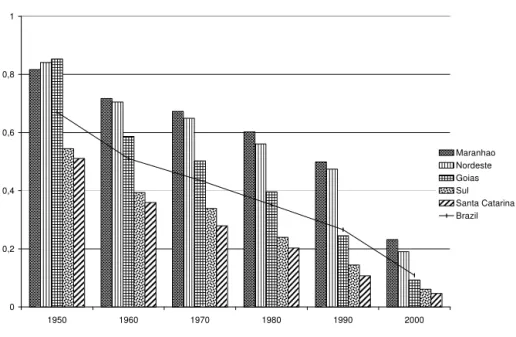
Observe that Figure 4 singles out some regions (Nordeste and Sul) and some States (Goias, Santa Catarina and Maranhão). On average for the country, non-educated people represented 67% of total population in 1950, a proportion that has fallen to 11% today. Needless to say, this remarkable aggre-gate performance makes strong regional disparities, even though all regions have indeed followed the same trend evolution. Noteworthy is the case of Nordeste which is the region that shows the steepest negative trend despite with the highest proportion of non-educated.
23See in Appendix.
Figure 4 –Trend of Brazilian with No Schooling
0 0,2 0,4 0,6 0,8 1
1950 1960 1970 1980 1990 2000
Maranhao Nordeste Goias Sul Santa Catarina Brazil
3.3. Trend of the Average Number of Years of Schooling
Table 526 reports on trend of Average Number of Years of Schooling (AYS). We see that, although
it remains weak compared to other relevant countries, the Brazilian AYS increases a lot during the considered period, from 1,34 reaching the level of 6,28 in 2000. Regional and state ranking is more stable through time here than was suggested by the Gini index. This is of course not a surprise since it is much more difficult to change substantially the average number of years of schooling.
Sudeste performs systematically better in terms of AYS on the considered period, except in the very beginning. This region appears quite unequal according to the AYS criterion (ranking at the second place in terms of AYS standard deviation), which was not the case when considering Education Gini. As it was already apparent from Education Gini comparison, Nordeste lags behind with an AYS of 4,8156 in 2000 even though it experienced the highest rate of increase among regions (+758%).
The weakest performance (in terms of increasing rate) occurs in Centro-Oeste with 146%. It owes his relative dynamism to Goias (with an increasing rate of 1168% between 1950 and 2000, the AYS goes from 0,5082 to 6,4421).
At the state level, despite the lowest increasing rate of 108 %, the best performance is achieved by Distrito Federal, where it is worth noting the AYS fell from 1950s to 1960s. It may correspond to the decision time which Brasilia has been designed as the Federal capital. That decreased may be related to the migration and to the civil construction labor force. Piaui stands unquestionably at the other extreme of the spectrum. Note interestingly that the trend of AYS is relatively similar between states in
Region Nordeste, and despite the same AYS, States of Sergipe and Bahia (respectively 1.99 and 1.91 in 1980s) incure stronger difference in Education Gini (respectively 0.73 and 0.79).
3.4. Trend of the Education Standard Deviation
In Table 6,27 we report another measure of the educational inequalities: the Education Standard
Deviation (ESD). This index is widely used presumably because it combines basic statistical and easily available measurements, even though it does not satisfy the conditions SI and DT.
It is defined as follows:
ESD=X i
q
pi(xi−x)2
The overall picture on the evolution of educational inequalities using this statistical index is differ-ent than the one obtained from Education Gini. According to the former index, educational inequalities increase on the half century, standard deviation growing from 2,55 to 4,57.
We make a few observations. First, there is strong convergence both between regions and between states.
Second, the most unequal regions and states are the ones with highest AYS and then Centro-Oeste and Sudeste: Distrito Federal and Rio de Janeiro are the most unequal States, however occurring with the lowest growth rate of the Education Standard Deviation on the considered period: +24% for Centro-Oeste and +17% for Sudeste.
Third, the lowest educational inequality is achieved by Nordeste (between 1950 and 1980 despite the highest growth rate on the considered period: +156%) and Norte (in 1990 and 2000).
Results clearly contrast with the one obtained from Education Gini. Looking carefully, Regions or states are also in inverted positions compared to the Average number of Years of Schooling.
4. LOOK BEYOND THE AVERAGE AND CONSEQUENCES ON BRAZILIAN WAGE
INEQUAL-ITY
4.1. Link between Education Gini and Average Number of Years of Schooling
Examining cross-state patterns of the distribution of education, we find that Education Gini declines as the average education level increases. That is, States or Regions with higher AYS are most likely to achieve an equitable education system as can be seen from Figure 5 below.28
This inverse relationship between Education Gini and AYS estimated from a panel is robust and found in every cross section between 1950 to 2000.
The panel regression results, reported in Table 7,29also indicate statistically significant evidence of this negative relation, whether we use variables stacked by dates or by states or whether we control for time-specific or state-specific factors, or whether we use fixed, between or random effect models.
These results have important policy implications. They imply that moving any person out of illit-eracy (or with at least one year of education) improves both education Gini and the level of education attainment. Also increasing AYS by one year reduces the Education Gini index by almost 0,0933.
27See in Appendix.
Figure 5 –Average Number of Years of Education – Education Gini – States – 1950–2000
EG = -0,0933*AYS + 0,8981 (-26,71) (85,11)
R2 = 0,8754
0,2 0,3 0,4 0,5 0,6 0,7 0,8 0,9 1
0 1 2 3 4 5 6 7 8 9
Average Number of Years of Schooling
E d u c a ti o n G in i DF 00 RJ 00 SP 00 DF 90 SC 60 SC 90 SC 80 PE 90 BA 80 PE 00 PB 90 PE 50 AM 90 AC 00 GO 60 RS 60 PI 50 RJ 90 RS 80 RS 90 GO 00 RJ 90 MT 00 SE 00 RS 00 SC 00 AM 00 AL 00 RR 90 RN 90
PI 90AL 90
DF 60 AP 50 CE 70 PB 80 AL 80 ES 60 PR 60 RJ 60 RS 70 RR 70 PI 60 GO 80 MS 80 AP 80 CE 60 AL 60 BA 90 RN 80 RR 60 AP 60 MA 50 RN 60
4.2. Link between Education Standard Deviation and Average Number of Years of
Schooling
Kuznets has suggested that it is an unavoidable characteristic of the development process that income inequality should exhibit a hump-shaped profile.30 Should it also be the case for educational
inequality? Is this claim confirmed by Brazilian data?
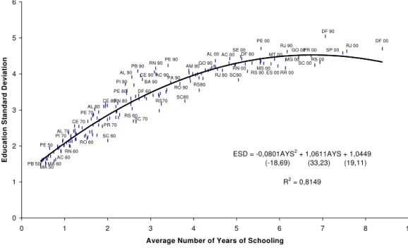
In Table 831 and Figure 6, we provide some econometric tests of this claim. For this, we regress
Education Standard Deviation and Average number of Years of Schooling assuming either a parabolic or a log fit.
Econometric results show that this parabolic-fit is significant using Within or GLS regression (but not using a Between regression). Hence, this relation becomes significant if we consider temporal
30Kuznets (1966): ”It seems plausible to assume that in the process of growth, the earlier periods are characterized by a balance
of counteracting forces that may have widened the inequality in the size distribution of total income for a while because of the rapid growth of the non-A [non-agricultural] sector and wider inequality within it. It is even more plausible to argue that the recent narrowing in income inequality observed in the developed countries was due to a combination of the narrowing inter-sectoral inequalities in product per worker, the decline in the share of property incomes in total incomes of households, and the institutional changes that reflect decisions concerning social security and full employment.”
Figure 6 –Average Number of Years of Education – Education Standard Deviation – States – 1950–2000
ESD = -0,0801AYS2 + 1,0611AYS + 1,0449 (-18,69) (33,23) (19,11)
R2 = 0,8149
0 1 2 3 4 5 6
0 1 2 3 4 5 6 7 8 9
Average Number of Years of Schooling
E d u c a ti o n S ta n d a rd D e v ia ti o n DF 00 RJ 00 SP 00 DF 90 RS 00 SC 00 PR 00 GO 00 RR 00 RJ 90 PE 00 RS 90 SC90 RS80 SC80 RS70 SC 70 RS 60 SC 60 PB 50 AC 60 MA 60 MA 50 RO 60 RN 60 PE 50 SE 00 DF 80 AC 00 RJ 80 MS 00 ES 00 RO 90 AL 00 AM 90 PE 90 RN 90 AC 90 PB 90 BA 90 CE 90 AL 90 PI 90 MT 00 MG 00 RN 00 GO 90 PE 80 RN 80 DF 60 AL 80 CE 80 CE 70 AL 70 PI 70 PE 70 PR 70 PA 90
fluctuations of the States around their average level. It seems to corroborate Thomas et al. (2001). Indeed a Brazilian Educational Kuznets curve does seem to emerge from our data, with a reversal point around 6,59.
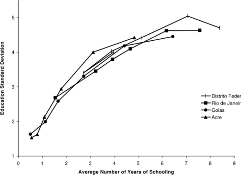
In fact from data, that reversal (inflection) point only occurs for Distrito Federal around 7 average number of years of schooling (between 1990 and 2000), as describing and should occurs soon for Rio de Janeiro, Goias (but also São Paulo) as showed in Figure 7. Concerning other states, a possible cause of that non-result may be that our temporal sample is not large enough to come across a U-Shaped inverse as the well known Kuznets curve or that Brazil is in the second phase of development, according the Education Kuznets curve.
While interpretation in logarithmic-fit is not clear (increasing Average number of Years of Schooling will infinitely increase Education inequality, measured by Education Standard Deviation), the Kuznets one is obvious.
For a state which has low schooling achievement, helping people to become educated may enlarge the Education Standard Deviation and the spread of education will be widened as people are getting higher educated.
Figure 7 –Average Number of Years of Education – Education Standard Deviation in selected States – 1950–2000
1 2 3 4 5
0 1 2 3 4 5 6 7 8 9
Average Number of Years of Schooling
E
d
u
c
a
ti
o
n
S
ta
n
d
a
rd
D
e
v
ia
ti
o
n
Distrito Federal Rio de Janeiro Goias Acre
a rise in inheritance inequality because well educated people leave a bequest while the poor devote their time to work and not to education (constrained by a threshold of minimal consumption). Trade-off between time allocated to education or work acts in favour of work for children of poor educated people. In such condition, increasing AYS can be due to the high part of the distribution, increasing such a way educational inequality.
Low educated people benefits from higher AYS as it increases. Trade-off between work and edu-cation acts now in favour of eduedu-cation for high and medium part of the distribution. More and more people continue one’s studies. This allows them to escape from their minimal present consumption through economic and educational perspective. In later stages, a increasing AYS is mainly due to an increasing education time of the whole population. Inequality is then clearly decreasing.
A political strategy consists then to attain this threshold as soon as possible.
4.3. Implications on Brazilian Wage Inequality
An interesting observation should be made after comparing the behavior of Education Gini and the Education Standard Deviation. In spite of schooling achievement (i.e. rise in average number of years of schooling), helping agents to be educated on the one hand increases Education Standard Deviation, on the other hand it decreases the Education Gini coefficient value. Nevertheless, Education Gini index seems to be more robust and appropriate to study disparities in educational distribution. Indeed, whatever the average number of years of schooling, an additional educational year provoke a diminishing of the Education Gini, than in terms of Education Standard Deviation, situation calls for previously high average number of years of schooling.
Brazil´s experience has resulted in periods in which reduction in schooling inequality coincided with rises in income inequality. As shown above, the variance of schooling has peaked with more recent cohorts in the country, suggesting that this component will contribute to declining earnings inequality in the future.32 Unambiguous improvements in the distribution of schooling, could lead to
decreased inequality in earnings. The fundamental reason is that earnings are likely to be a convex function of schooling, the log-linear wage equation being just one simple example of such convexity.
5. CONCLUSION
In this paper, we provide a statistical description of Brazilian human capital dispersion, in time, across regions and states. Our analysis highlights several stylized facts.
First, there is in Brazil a strong reduction of educational inequalities as measured by Education Gini index. Despite the fact that this trend is shared by all regions and states, disparities remain important, reflecting educational geographical disparities and economic performance. A three parts picture of Brazil seems to emerge: Regions Norte and Nordeste with results showing a distinct improvement, but remaining weak. They suffer from unfavorable initial conditions inherited from the past. Regions and Sul correspond to regions most evenly distributed. Centro-Oeste exhibits high heterogeneity between states.
Second, we have shown that there is a strong diminution of educational inequalities as far as school-ing achievement is concerned. In each state, the average years of schoolschool-ing increased notably from 1,34 to 6,28 between year 1950 and year 2000 in Brazil.
Third, we have shown that there is a significant negative link between Education Gini and the average education length: higher education achievement leads to a more equitable distribution.
Finally, we have shown that Brazilian data are consistent with an Education Kuznets curve if we consider the education standard deviation, though evidence is yet somewhat weak.
However, there were a number of education reforms in Brazil over the period under analysis. Also, as long as education increases, the issue of quality of education gains importance. We obviously are not able to measure that point in our paper. It could be interesting to study more carefully the impact a such reforms on access to education and wages determination.
32Remember that standard deviation of schooling tends to follow an inverted-Upattern in relation to mean schooling, with a
Bibliography
Acemoglu, D. (1995). Reward structures and the allocation of talent.European Economic Review, 39(1):17– 33.
Aghion, P. & Bolton, P. (1997). A theory of trickle-down growth and development. Review of Economic Studies, 64(2):151–72.
Alesina, A. & Perotti, R. (1996). Income distribution, political instability, and investment. European Economic Review, 40(6):1203–1228.
Alesina, A. & Rodrik, D. (1994). Distributive politics and economic growth. The Quarterly Journal of Economics, 109(2):465–90.
Atkinson, A. B. & Bourguignon, F. (1998). Measurement of inequality. InHandbook of Income Distribution. North-Holland.
Barro, R. J. (1991). Economic growth in a cross section of countries. The Quarterly Journal of Economics, 106(2):407–43.
Barro, R. J. & Lee, J.-W. (2001). International data on educational attainment: Updates and implications.
Oxford Economic Papers, 53(3):541–63.
Barros, R. P. d., Henriques, R., & Mendonça, R. (2002). Pelo fim das décadas perdidas: Educação e desenvolvimento sustentado no Brasil. TD 857, IPEA.
Barros, R. P. d. & Mendonça, R. (1997). Investimentos em educação e desenvolvimento econômico. TD 525, IPEA.
Barros, R. P. d. & Mendonça, R. (1998). O impacto de três inovações institucionais na educação brasileira. TD 556, IPEA.
Becker, G. S. & Barro, R. J. (1988). A reformulation of the economic theory of fertility. The Quarterly Journal of Economics, 103(1):1–25.
Becker, G. S., Murphy, K. M., & Tamura, R. (1990). Human capital, fertility, and economic growth.Journal of Political Economy, 98(5):S12–37.
Benabou, R. (1996). Inequality and growth. Macroeconomics Annual 11, NBER.
Benhabib, J. & Rustichini, A. (1996). Social conflict, growth and income distribution.Journal of Economic Growth, 1(1).
Blom, A., Holm-Nielsen, L., & D., V. (2001). Education, earning and inequality in brazil: 1982–98. impli-cation for eduimpli-cation policy. Working Paper 2686, World Bank Policy Research.
Bowman, K. S. (1997). Should the kuznets effect be relied on to induce equalizing growth: Evidence from post-1950 development.World Development, 25(1):127–143.
Ferreira, S. G. (2003). Mobilidade intergeracional de educação no Brasil. Pesquissa e Planejamento Econômico, 33(3).
Galor, O. & Moav, O. (2002). Natural selection and the origin of economic growth. The Quarterly Journal of Economics, 117(4):1133–1191.
Hussar, W. & Sonnenberg, W. (2000). Trends in disparities in school district level expenditures per pupil. Technical Report 20, NCES.
Lam, D. (1999). Generating extreme inequality: Schooling, earnings and intergenerational transmission of human capital in South Africa and Brazil. Report 99–439, Population Studies Center.
Lam, D. & Levison, D. (1991). Declining inequality in schooling in Brazil and its effects on inequality in earnings.Journal of Development Economics, 37(1–2):199–225.
Maas, J. & Criel, C. (1982). Distribution of primary school enrollments in Eastern Africa. Technical Report WP 511, World Bank Staff.
Maddison, A. & Associates (1992).The Political Economy of Poverty, Equality and Growth. Oxford University Press.
Psacharopoulos, G. & Arriagada, A. M. (1986). The education attainment of the labor force: An interna-tional comparison. Technical Report EDT 38, World Bank Report.
Saint-Paul, G. & Verdier, T. (1993). Education, democracy and growth. Journal of Development Economics, 42(2):399–407.
A. INDICATORS USED TO QUANTIFY EDUCATION
Several indicators have been proposed to quantify alternative aspects of education. Some make use of flow variables such as the enrollment rate to different schooling levels (used mainly in relation with the primary and secondary education) as indicators of human accomplishment (e.g. Barro (1991)). These variables measure access flow to education and therefore do not take into account the schooling level achieved. These do not seem particularly appropriate measure to use in growth analysis where the stock of human capital is the main focus.
The difficulty with using stock measures such as achievement levels quantified by the average num-ber of years of schooling, is due to missing. Thanks to Psacharopoulos and Arriagada (1986) and to Barro (1991), Barro and Lee (2001), robust international data about the average number of years of schooling are now available.
In recent years however, the emphasis has shifted toward quality rather than quantity indices of education. There are two main approaches:
i A first approach is concerned with measuring factors and resources used in the production of ed-ucation. For instance the ration of professor to student, the average income earned by teachers, the number of libraries or books made available to students or public and private expenditures per student. But international comparisons using these measures are difficult because they cru-cially depend on countries’ education system. Furthermore, high education budget does not nec-essarily imply quality of education of quality and by no means reveals anything on who accesses to education.
ii A second approach uses the international Test Score of Cognitive Performance. This test makes possible international comparisons of schooling achievements between students of the same age group. Subjects are common in sciences and mathematics and this test is run by the International Association for Evaluation of Educational Achievement (IEA) and by the International Assessment of Education Progress (IEAP). However, these recent efforts yet only cover a dozen of countries, mostly industrial, which limits their usefulness. Furthermore they are not fully time consistent. Another kind of indicators is turning up. Indeed, in some studies indicators of disparities have been counted from various data; such as enrollment rates, financial rates, average expenditure per student or schooling achievement. For instance, Maas and Criel (1982) make use of the Gini Index on the enrollment rates for 16 East African countries. Hussar and Sonnenberg (2000) analyze the per student schooling expenditure disparities between US states and within states using among others coefficient of variation, Gini coefficient, Theil coefficient. Thomas et al. (2001) consider a Gini index on schooling achievement of population aged over fifteen between 1960 and 1990 for 85 countries.
B. DESIRABLE PROPERTIES OF THE INEQUALITY INDICES
The idea of inequality refers to several domains: income, health, education. . . An inequality index is a scalar summary of the dispersion of the distribution and as such necessarily disregards a lot of important pieces of data about the distribution.
There are many ways of measuring inequality, all of which have some intuitive or mathematical appeal. However, many apparently sensible measures behave in perverse fashions. For example, the variance, which must be one of the simplest measures of inequality, is not independent of the income scale:33 simply doubling all incomes would register a quadrupling of the estimate of income inequality.
We list several properties with the axiomatic approach that a perfect inequality index would have to
satisfy. Of course, such a perfect indicator does not exist and depending on the data at your disposal, on the analyses framework, we will privilege one indicator rather than another one.
i Pigou-Dalton Transfer Condition (PDT): transfers of benefits from the “rich” to the “poor” do not have to reverse the ranking. Most measures in the literature, including the Generalized Entropy class, the Atkinson class and the Gini coefficient, satisfy this principle, with the main exception of the logarithmic variance and the variance of logarithms.
ii Translation Invariance (TI): the inequality is unchanged when all individual benefits increase by the same amount.
iii Scale Invariance (SI): the inequality is unchanged when all individual benefits increase in the same proportion. Again most standard measures pass this test except the variance sincevar(λy) =
λ2var(y).
iv Subgroup Consistency (SC): when only a subgroup of agents is affected by a change in their benefits, the overall inequality moves in the same direction as this subgroup inequality.
v Diminishing Transfers (DT): a transfer from rich to poor decreases inequality more when it is made at the lower tail of the distribution than when it is made at the upper tail.
Generalized entropy: c(c1
−1)
P
i
pi xxi c
−1
wherecis a given parameter. Forc <2, it satisfies all above conditions, except TI. Note that ifc = 0, the formula becomes:
P
i
piln xxi
and ifc = 1, it becomes the Theil Index:
P
i pixi
x ln
xi
x
. Notice that for allc < 1, it is ordinal equivalent to the Kolm-Atkinson Index withε= 1−c.
Table 1 –Regression: Earnings Function
Brazil Norte Nordeste Sudeste Sul Centro-Oeste Constant 5,452
(11,12)
5,726 (7,81)
6,447 (13,01)
5,093 (8,1) 5,482 (6,89)
5,239 (9,38) e0 0,215 (3,75) 0,052
(0,07)
0,03 (3,62) 0,245 (3,06)
0,41 (2,15)
0,219 (3,17) e1 -0,578
(-3,91)
-0,29 (-1,8) -0,173 (-3,94)
-0,479 (-3,02)
-0,577 (-2,13)
-0,98 (-3,3) e3 0,949 (3,49) 0,795
(1,45)
0,564 (3,64)
0,477 (2,88)
0,505 (1,86)
1,459 (2,93) e4 -0,526
(-3,49)
-0,467 (-1,49)
-0,262 (-3,75)
-0,2 (-2,86)
-0,254 (-1,78)
-0,67 (-2,84) e5 0,578 (4,62) 1,179
(2,47)
0,3 (4,63)
0,125 (3,36)
0,3 (2,35)
0,743 (4,12) AdjR2 0,8784 0,7054 0,8833 0,8241 0,699 0,8551
Table 2 –Trend of Education Gini of Brazilians 5 years and over – Region – State (1950–2000)
Regions States 1950 1960 1970 1980 1990 2000
Brazil 0,7868 0,6246 0,6485 0,5830 0,5307 0,4031
Norte
Acre 0,8807 0,7743 0,7929 0,7442 0,6510 0,4970
Amapa 0,8294 0,6696 0,6344 0,5874 0,5178 0,4279
Rondonia 0,7788 0,6656 0,7052 0,6344 0,5385 0,4189
Roraima 0,8355 0,7268 0,6235 0,6077 0,5282 0,3779
Amazonas 0,8506 0,7020 0,7191 0,6541 0,5669 0,4353
Para 0,7661 0,6367 0,6571 0,6347 0,5664 0,4403
NORTE 0,7989 0,6659 0,6823 0,6439 0,5662 0,4366
Centro-Oeste
Mato-Grosso do Sul 0,5874 0,5036 0,4069
Mato-Grosso 0,7726 0,6302 0,6758 0,6252 0,5246 0,4109
Goias 0,9115 0,7031 0,7035 0,6164 0,5126 0,3829
Tocantins 0,6352 0,4494
Distrito Federal 0,5275 0,5432 0,5510 0,4789 0,4065 0,3142
CENTRO-OESTE 0,6714 0,6738 0,6851 0,5969 0,5023 0,3847
Sudeste
Minas Gerais 0,7988 0,6366 0,6448 0,5577 0,5131 0,3921
Espirito Santo 0,8044 0,6387 0,6493 0,5556 0,5056 0,3900
Rio de Janeiro 0,7584 0,4847 0,5155 0,4799 0,4176 0,3427
Sao Paulo 0,6741 0,5102 0,5361 0,4927 0,4323 0,3418
SUDESTE 0,7391 0,5496 0,5707 0,5111 0,4558 0,3585
Sul
Parana 0,7831 0,6276 0,6478 0,5493 0,4842 0,3717
Santa Catarina 0,6525 0,5434 0,5124 0,4526 0,4009 0,3417
Rio Grande do Sul 0,6586 0,5081 0,5097 0,4557 0,4134 0,3410
SUL 0,6916 0,5617 0,5705 0,4931 0,4383 0,3526
Nordeste
Maranhao 0,8786 0,7789 0,7991 0,7544 0,6949 0,5116
Piaui 0,9253 0,8107 0,8364 0,7597 0,7209 0,5182
Ceara 0,9180 0,7533 0,8144 0,7306 0,6936 0,4650
Rio Grande do Norte 0,8921 0,7267 0,7640 0,6874 0,6652 0,4648
Paraiba 0,9128 0,7687 0,8010 0,7365 0,7140 0,4998
Pernambuco 0,9009 0,7319 0,7551 0,6874 0,6362 0,4630
Alagoas 0,9199 0,7902 0,8243 0,7713 0,7203 0,5148
Sergipe 0,8803 0,7471 0,7917 0,7261 0,6597 0,4761
Bahia 0,8873 0,7500 0,7884 0,7887 0,6743 0,4831
NORDESTE 0,9018 0,7597 0,7930 0,7302 0,6805 0,4856
Maximum State 0,9253 0,8107 0,8364 0,7887 0,7209 0,5182
Etat State Piaui Piaui Piaui Bahia Piaui Piaui
Max Region 0,9018 0,7597 0,7930 0,7302 0,6805 0,4856
Region Max Nordeste Nordeste Nordeste Nordeste NordesteNordeste
Min State 0,5275 0,4847 0,5097 0,4526 0,4009 0,3142
State Min* DF RJ RGS SC DF DF
Min Region 0,6714 0,5496 0,5705 0,4931 0,4383 0,3526
Region Min CO Sudeste Sul Sul Sul Sul
Table 3 –Trend of Education Gini with No Schooling of Brazilians 5 year and over (1950–2000)
Regions States 1950 1960 1970 1980 1990 2000
Brazil Total - Brésil 0,3531 0,3222 0,3772 0,3571 0,3606 0,3302
Norte
Acre 0,3732 0,3150 0,3762 0,3676 0,3749 0,3573
Amapa 0,4023 0,3371 0,3596 0,3518 0,3391 0,3350
Rondonia 0,3767 0,2992 0,3687 0,3454 0,3534 0,3441
Roraima 0,3789 0,3392 0,3427 0,3596 0,3352 0,2993
Amazonas 0,3907 0,3407 0,4062 0,3749 0,3529 0,3231
Para 0,3637 0,3234 0,3883 0,3726 0,3772 0,3523
NORTE 0,3718 0,3279 0,3909 0,3710 0,3688 0,3426
Centro-Oeste
Mato Grosso 0,3728 0,3370 0,3893 0,3596 0,3585 0,3292
Goias 0,3971 0,3547 0,4041 0,3647 0,3546 0,3200
Distrito Federal 0,3051 0,3427 0,3752 0,3532 0,3195 0,2834
CENTRO-OESTE 0,3297 0,3529 0,4074 0,3701 0,3582 0,3210
Sudeste
Minas Gerais 0,3518 0,3159 0,3697 0,3483 0,3557 0,3275
Espirito Santo 0,3791 0,3186 0,3786 0,3501 0,3501 0,3242
Rio de Janiero 0,3502 0,2988 0,3548 0,3470 0,3319 0,3008
São Paulo 0,3286 0,2957 0,3560 0,3486 0,3458 0,2986
SUDESTE 0,3443 0,3093 0,3658 0,3512 0,3490 0,3093
Sul
Parana 0,3631 0,3270 0,3725 0,3539 0,3618 0,3169
Santa Catarina 0,2893 0,3061 0,3233 0,3131 0,3291 0,3097
Rio Grande do Sul 0,3191 0,2957 0,3331 0,3229 0,3344 0,3054
SUL 0,3232 0,3121 0,3503 0,3334 0,3436 0,3108
Nordeste
Maranhão 0,3378 0,3157 0,3860 0,3824 0,3910 0,3643
Piaui 0,3831 0,3547 0,4130 0,3877 0,3988 0,3723
Ceara 0,4043 0,3525 0,4309 0,3904 0,3987 0,3555
Rio Grande do Norte 0,3643 0,3197 0,3775 0,3680 0,3918 0,3585
Paraiba 0,3749 0,3382 0,4110 0,3881 0,4044 0,3691
Pernambuco 0,3760 0,3407 0,3955 0,3809 0,3746 0,3574
Alagoas 0,3891 0,3448 0,4162 0,3897 0,3913 0,3752
Sergipe 0,3964 0,3535 0,4296 0,3852 0,3861 0,3717
Bahia 0,3714 0,3402 0,4114 0,3877 0,3943 0,3629
NORDESTE 0,3808 0,3430 0,4097 0,3860 0,3923 0,3647
Max State 0,4043 0,3547 0,4309 0,3904 0,4044 0,3752
State Max Ceara Goias Ceara Ceara Paraiba Alagoas
Max Region 0,3808 0,3529 0,4097 0,3860 0,3923 0,3647
Region Max Nordeste CO Nordeste Nordeste NordesteNordeste
Min State 0,2893 0,2957 0,3233 0,3131 0,3195 0,2834
State Min SC RS SC SC DF DF
Min Region 0,3232 0,3093 0,3503 0,3334 0,3436 0,3093
Region Min Sul Sudeste Sul Sul Sul Sudeste
Table 4 –Trend of No Schooling of Brazilian 5 years and over – Region – State (1950–2000)
Regions States 1950 1960 1970 1980 1990 2000
Brazil 0,6705 0,5103 0,4357 0,3514 0,2661 0,1089
Norte
Acre 0,8097 0,7086 0,6680 0,5955 0,4416 0,2174
Amapa 0,7146 0,5450 0,4291 0,3634 0,2704 0,1398
Rondonia 0,6452 0,5493 0,5331 0,4414 0,2862 0,1141
Roraima 0,7351 0,6229 0,4272 0,3873 0,2904 0,1123
Amazonas 0,7547 0,6035 0,5269 0,4467 0,3307 0,1657
Para 0,6325 0,5022 0,4394 0,4178 0,3038 0,1359
NORTE 0,6800 0,5463 0,4784 0,4338 0,3128 0,1431
Centro-Oeste
Mato-Grosso do Sul 0,3564 0,2236 0,1251
Mato-Grosso 0,6374 0,4782 0,4692 0,4144 0,2621 0,1115
Goias 0,8532 0,5868 0,5024 0,3961 0,2448 0,0926
Tocantins 0,4162 0,1610
Distrito Federal 0,3201 0,3608 0,2815 0,1942 0,1278 0,0430
CENTRO-OESTE 0,5097 0,5429 0,4686 0,3601 0,2245 0,0938
Sudeste
Minas Gerais 0,6896 0,5287 0,4365 0,3214 0,2443 0,0961
Espirito Santo 0,6850 0,5316 0,4356 0,3162 0,2393 0,0973
Rio de Janeiro 0,6282 0,3127 0,2490 0,2035 0,1283 0,0599
Sao Paulo 0,5145 0,3645 0,2796 0,2212 0,1322 0,0615
SUDESTE 0,6021 0,4098 0,3230 0,2465 0,1640 0,0713
Sul
Parana 0,6594 0,4985 0,4388 0,3025 0,1918 0,0801
Santa Catarina 0,5110 0,3591 0,2794 0,2031 0,1069 0,0463
Rio Grande do Sul 0,4985 0,3254 0,2648 0,1960 0,1187 0,0506
SUL 0,5443 0,3934 0,3389 0,2396 0,1442 0,0607
Nordeste
Maranhao 0,8166 0,7170 0,6728 0,6024 0,4991 0,2317
Piaui 0,8789 0,7778 0,7213 0,6075 0,5358 0,2325
Ceara 0,8624 0,7141 0,6738 0,5580 0,4903 0,1699
Rio Grande do Norte 0,8303 0,6467 0,6208 0,5054 0,4495 0,1657
Paraiba 0,8717 0,6985 0,6622 0,5694 0,5198 0,2072
Pernambuco 0,8412 0,6746 0,5949 0,4951 0,4184 0,1643
Alagoas 0,8689 0,7637 0,6991 0,6253 0,5406 0,2235
Sergipe 0,8017 0,6619 0,6349 0,5545 0,4457 0,1662
Bahia 0,8206 0,6857 0,7085 0,5732 0,4622 0,1887
NORDESTE 0,8413 0,7052 0,6493 0,5606 0,4742 0,1904
Max State 0,8789 0,7778 0,7213 0,6253 0,5406 0,2325
State Max Piaui Piaui Piaui Alagoas Alagoas Piaui
Max Region 0,8413 0,7052 0,6493 0,5606 0,4742 0,1904
Region Max Nordeste Nordeste Nordeste Nordeste NordesteNordeste
Min State 0,3201 0,3127 0,2490 0,1942 0,1069 0,0430
State Min DF RJ RJ DF SC DF
Min Region 0,5097 0,3934 0,3230 0,2396 0,1442 0,0607
Region Min CO Sul Sudeste Sul Sul Sul
Table 5 –Trend of Average Number of Years of Schooling of Brazilians 5 years and over – Region – State (1950–2000)
Regions States 1950 1960 1970 1980 1990 2000
Brazil 1,3461 1,8011 2,3902 3,2366 4,3623 6,2779
Norte
Acre 0,5550 0,7904 1,0904 1,7887 3,1211 4,8404
Amapa 0,8475 1,4604 2,2767 3,0556 4,3364 5,5453
Rondonia 1,1272 1,5192 1,8024 2,1875 3,6778 5,6272
Roraima 0,9506 1,2639 2,2492 2,8624 4,2721 6,1357
Amazonas 0,8334 1,2478 1,7546 2,5403 3,8869 5,5645
Para 1,1696 1,5397 1,9940 2,5448 3,4655 5,3557
NORTE 1,0298 1,4082 1,8833 2,4945 3,6182 5,4505
Centro-Oeste
Mato-Grosso do Sul 2,8998 4,5086 5,7983
Mato-Grosso 1,2725 1,6493 1,7882 2,5383 4,0478 5,8802
Goias 0,5082 1,1255 1,6626 2,7281 4,4219 6,4421
Tocantins 2,6515 5,2013
Distrito Federal 3,9786 2,7186 3,8934 5,1189 7,0641 8,3872
CENTRO-OESTE 2,6666 1,3621 1,9378 3,1041 4,8086 6,5575
Sudeste
Minas Gerais 1,1428 1,5814 2,1991 3,1814 4,0884 6,1413
Espirito Santo 0,9796 1,4908 2,2134 3,3736 4,3855 5,9597
Rio de Janeiro 1,5399 3,2240 3,9264 4,6683 6,1743 7,5609
Sao Paulo 2,1922 2,5673 3,3584 4,2152 5,5420 7,4686
SUDESTE 1,6609 2,3725 3,1160 4,0189 5,2580 7,0954
Sul
Parana 1,2469 1,6340 2,0466 3,1983 4,5540 6,7343
Santa Catarina 1,7530 2,0028 2,6597 3,7980 5,0425 6,8176
Rio Grande do Sul 1,8761 2,5988 3,2517 4,1286 5,2505 6,9348
SUL 1,6828 2,1475 2,6527 3,6973 4,9419 6,8356
Nordeste
Maranhao 0,5613 0,7567 1,0460 1,6153 2,4478 4,1801
Piaui 0,4614 0,6723 0,9604 1,6511 2,4111 3,9125
Ceara 0,4824 0,8699 1,2298 1,9426 2,7644 4,9521
Rio Grande do Norte 0,5671 1,1069 1,4071 2,2328 3,1152 4,9736
Paraiba 0,4439 0,9113 1,2079 1,9488 2,7007 4,4752
Pernambuco 0,6518 1,1432 1,6719 2,4414 3,4035 5,5676
Alagoas 0,4725 0,7433 1,0895 1,6959 2,5633 4,5058
Sergipe 0,5975 0,9147 1,2369 1,9910 3,0846 5,0933
Bahia 0,6176 0,9884 1,3293 1,9081 2,8080 4,8241
NORDESTE 0,5614 0,9179 1,3030 1,9720 2,8361 4,8156
Max State 3,9786 3,2240 3,9264 5,1189 7,0641 8,3872
State Max DF RJ RJ DF DF DF
Max Region 2,6666 2,3725 3,1160 4,0189 5,2580 7,0954
Region Max CO Sudeste Sudeste Sudeste Sudeste Sudeste
Min State 0,4439 0,6723 0,9604 1,6153 2,4111 3,9125
State Min Paraiba Piaui Piaui Maranhão Piaui Piaui
Min Region 0,5614 0,9179 1,3030 1,9720 2,8361 4,8156
Region Min Nordeste Nordeste Nordeste Nordeste NordesteNordeste
Table 6 –Trend of Education Standard Deviation of Brazilian 5 years and over – Region – State (1950– 2000)
Regions States 1950 1960 1970 1980 1990 2000
Brazil 2,5524 2,6595 3,1703 3,6296 4,3242 4,5703
Norte
Acre 1,5320 1,6251 2,1312 2,9432 4,0028 4,4260
Amapa 1,9285 2,2728 2,8703 3,4061 4,1005 4,3061
Rondonia 2,1263 2,2050 2,7084 2,7937 3,7337 4,2942
Roraima 2,1325 2,1956 2,7864 3,3637 4,1143 4,1680
Amazonas 1,9967 2,1765 2,7754 3,3248 4,0946 4,3538
Para 2,1300 2,2485 2,7365 3,2232 3,7696 4,3074
NORTE 2,0669 2,2039 2,7292 3,2154 3,8802 4,3217
Centro-Oeste
Mato-Grosso do Sul 3,3150 4,2041 4,2809
Mato-Grosso 2,3291 2,3091 2,5855 3,1584 3,9744 4,4099
Goias 1,6311 1,9922 2,5874 3,3072 4,1862 4,4532
Tocantins 3,3756 4,2781
Distrito Federal 4,0037 3,4062 4,0317 4,4184 5,0470 4,7055
CENTRO-OESTE 3,6789 2,2154 2,8559 3,5922 4,4282 4,5470
Sudeste
Minas Gerais 2,2530 2,3920 2,9478 3,4257 4,0012 4,3916
Espirito Santo 2,0161 2,2975 2,9619 3,5602 4,1299 4,2194
Rio de Janeiro 2,6865 3,4576 3,7977 4,1013 4,6236 4,6353
Sao Paulo 3,0947 3,0352 3,5014 3,8748 4,4031 4,5867
SUDESTE 2,7547 3,0035 3,4721 3,8462 4,4086 4,5772
Sul
Parana 2,3570 2,3989 2,7723 3,3863 4,1346 4,5061
Santa Catarina 2,2985 2,1503 2,6744 3,2481 3,8387 4,2454
Rio Grande do Sul 2,5508 2,6913 3,1643 3,5475 4,0704 4,3225
SUL 2,4666 2,5373 2,9758 3,4545 4,0610 4,3768
Nordeste
Maranhao 1,5090 1,5841 2,0888 2,7505 3,5398 4,0139
Piaui 1,5770 1,7120 2,1637 2,8399 3,7115 3,8929
Ceara 1,6204 1,9655 2,5561 3,0950 3,9519 4,2460
Rio Grande do Norte 1,6339 2,0062 2,5022 3,1906 4,1565 4,2723
Paraiba 1,4885 1,8731 2,4118 3,1646 4,0824 4,2182
Pernambuco 1,9353 2,2871 2,8740 3,4618 4,2383 4,7089
Alagoas 1,5918 1,8302 2,3623 3,0163 3,9152 4,3669
Sergipe 1,6413 1,8413 2,4409 3,1243 4,0521 4,4858
Bahia 1,7253 2,0169 2,5465 3,0992 3,8473 4,3022
NORDESTE 1,6912 1,9677 2,5292 3,1326 3,9377 4,3371
Max State 4,0037 3,4576 4,0317 4,4184 5,0470 4,7089
State Max DF RJ DF DF DF DF
Max Region 3,6789 3,0035 3,4721 3,8462 4,4282 4,5772
Region Max CO Sudeste Sudeste Sudeste CO CO
Min State 1,4885 1,5841 2,0888 2,7505 3,3756 3,8929
State Min Paraiba Maranhão Maranhão Maranhão Tocantins Piaui
Min Region 1,6912 1,9677 2,5292 3,1326 3,8802 4,3217
Region Min Nordeste Nordeste Nordeste Nordeste Norte Norte
Assessing
Brazilian
Educational
Inequ
alities
Average Years of Schooling -0,0933** -0,0719* -0,914** -0,0707** -0,0968** -0,0745** (-26,71) (-6,89) (-27,28) (-30,85) (-16,98) (-33) Intercept(s) Between Effects Between Effects
Nordeste 0,9292 Maranhão 0,9497
Year 1950 0,9007 Piaui 0,9389
Ceara 0,9127 Rio Grande do Norte 0,9078
Year 1960 0,9380 Paraiba 0,9192
Pernambuco 0,9151 Alagoas 0,9286
Year 1970 0,8902 Sergipe 0,9312
Bahia 0,9108
Year 1980 0,8840 Centro-Oeste 0,9557
Mato Grosso do Sul -Mato Grosso 0,9115
Year 1990 0,8735 Goias 0,9068
Tocantins -Distrito Federal 0,9447
Year 2000 0,9314 Sudeste 0,8596
Minas Gerais 0,8974 Espiritos Santos 0,9137 Rio de Janeiro 0,8342 São Paulo 0,8267 Sul 0,9083 Parana 0,8991 Santa Catarina 0,8807 Rio Grande do Sul 0,8769 Norte 0,9235 Acre 0,9539 Amapa 0,9185 Rondonia 0,9418 Roraima 0,9419 Amazonas 0,9306 Para 0,9035
Within Between Overall Within Between Overall Adjusted R-squared 0,8282 0,9223 0,8754 0,8823 0,9202 0,8754 Included Observations 27 States 6 (1950, 60, 70, 80, 90, 00)
Number of cross-sections 6 (1950, 60, 70, 80, 90, 00) 27 States
Total panel observations 155 155
torz-statistics in parenthesis. * significant at the 0,2 percent level. ** significant at the 0,1 percent level.
RBE
Rio
de
Janeiro
v.
62
n.
1
/
p.
31–56
Jan-Mar
Table 8 –Log and Parabolic Regression: Education Standard Deviation – Average Number of Years of Schooling – Brazil – 1950–2000
Parabolic-fit Logaritmic-fit
R-sq Random 0,8149 Observations 155 R-sq Random 0,9229 Observations 155
Within 0,8896 Groups 27 Within 0,9634 Groups 27
Between 0,8896 Between 0,8395
GLS Regresion
ESD Coef z
GLS Regresion
ESD Coef z
AYS 1,0611 33,23 ln (AYS) 1,3343 55,67
AY S2 -0,0801 -18,69 Cons 2,0551 52,3
Cons 1,0449 19,11
Within Regression
ESD Coef t
Within Regression
ESD Coef t
AYS 1,0866 35,87 ln (AYS) 1,3606 57,81
AY S2 -0,0824 -20,37 Cons 2,0441 84,1
Cons 1,0026 20,33
Between Regression
ESD Coef t
Between Regression
ESD Coef t
AYS 0,3189 1,60 ln (AYS) 0,9872 11,43
AY S2 -0,0132 -0,46 Cons 2,3574 29,6
Cons 2,0963 8,30
Table 9 –Abbreviation of States
Regions States Abbreviation
Norte
Acre AC
Amapa AP
Amazonas AM
Para PA
Rondonia RO
Roraima RR
Centro Oeste
Distrito Federal DF
Goias GO
Mato Grosso MT
Mato Grosso do Sul MS
Tocantins TO
Sudeste
Espiritos Santos ES
Minas Gerais MG
Rio de Janeiro RJ
São Paulo SP
Sul
Parana PR
Rio Grande do Sul RS
Santa Catarina SC
Nordeste
Alagoas AL
Bahia BA
Ceara CE
Maranhão MA
Paraiba PB
Pernambuco PE
Piaui PI
Rio Grande do Norte RN