Pesqui. Oper. vol.33 número2

(1)

GLOBAL OPTIMIZATION OF CAPACITY EXPANSION AND FLOW ASSIGNMENT IN MULTICOMMODITY NETWORKS

Ricardo Poley Martins Ferreira

1*

_{, Henrique Pacca Loureiro Luna}

2

_,

Philippe Mahey

3

_{and Mauricio Cardoso de Souza}

4

Received December 9, 2011 / Accepted January 22, 2013

ABSTRACT.This paper describes an exact algorithm to solve a nonlinear mixed-integer programming model due to capacity expansion and flow assignment in multicommodity networks. The model combines continuous multicommodity flow variables associated with nonlinear congestion costs and discrete decision variables associated with the arc expansion costs. After establishing precise correspondences between a mixed-integer model and a continuous but nonconvex model, an implicit enumeration approach is derived based on the convexification of the continuous objective function. Numerical experiments on medium size instances considering one level of expansion are presented. The results reported on the performance of the proposed algorithm show that the approach is efficient, as commercial solvers were not able to tackle the instances considered.

Keywords: capacity expansion, flow assignment, global optimization, implicit enumeration, multicom-modity flow problems.

1 INTRODUCTION

We consider a model for the joint problem of capacity expansion and flow assignment in multi-commodity flow networks which takes into account congestion effects. The resulting optimiza-tion problem relies on the combinaoptimiza-tion of two conflicting criteria: the expansion and the con-gestion cost functions. Capacity expansion cost functions are discrete as only a finite number of capacity sizes are available. On the other hand, congestion cost functions are nonlinear convex increasing functions as they try to capture queueing effects on the network [3, 4, 18, 23]. For

*Corresponding author

1Departamento de Engenharia Mecˆanica, Universidade Federal de Minas Gerais – UFMG, Brazil. Phone: +55(31) 3409-3503. E-mail: poley@demec.ufmg.br

2Instituto de Computação, Universidade Federal de Alagoas – UFAL, Maceió, Brazil. E-mail: henrique.luna@pq.cnpq.br

3LIMOS UMR 6158 CNRS, Université Blaise Pascal, Clermont-Ferrand, France. E-mail: philippe.mahey@isima.fr 4Departamento de Engenharia de Produção, Universidade Federal de Minas Gerais – UFMG, Brazil.

(2)

instance, Ishfaq & Sox [18], in the context of an intermodal hub network, deal with shipment delays due to limited resources at logistics hubs for measuring service performance. The authors conducted a study of strategies to integrate hub operation queuing model and the hub location-allocation model on a 25-city road-rail intermodal logistics network. Our aim is to study the general multicommodity flow problem under such assumptions, with no particular application in mind.

Typically, the two decision levels of capacity expansion and flow assignment are decoupled to treat the corresponding difficulties separately, and few works, at least those considering queue-ing effects, have been done on the joint optimization problem. Gerla & Kleinrock [14] stated the general Capacity and Flow Assignment problem (CFA), decomposed it into simpler subprob-lems, and then suggested a heuristic procedure that alternates a capacity assignment phase with a flow assignment phase. Similar approaches have been proposed in successive papers by Gavish and co-authors [11, 12] and Gerlaet al.[15]. Most of that literature concerns heuristic proce-dures, but the paper by Maheyet al.[20] is an exception for this rule, showing that a generalized Benders decomposition method can find exact solutions for the CFA problem.

The capacity expansion problem is a special case of CFA where initial capacities are already in-stalled on each arc of the network. Given a traffic requirement matrix between origin-destination pairs, the problem consists in jointly deciding which arc capacities, if any, should be expanded and the flow assignment leading to a feasible routing that minimizes expansion and congestion costs. Thus, the problem results in finding a trade-off between investment and routing costs.

Luna & Mahey [19] modeled the capacity expansion and flow assignment as a piecewise con-vex multicommodity flow problem. Congestion is modeled by a concon-vex increasing function for a given capacity and, at given breakpoints, which represents the maximum tolerable congestion for the users (thus strictly lower than the available capacity), expansion to a higher capacity is de-cided, decreasing the marginal congestion cost in a discontinuous way. The combinatorial nature of the problem, related to arc expansion decisions, is therefore embedded in a continuous objec-tive function that encompasses congestion and investment costs. The resulting objecobjec-tive function is continuous, but it is nonconvex and nonsmooth. Mahey and Souza [22] derived local optimal-ity conditions for the model proposed in [19]. By exploiting complete optimaloptimal-ity conditions for local minima, Souzaet al.[25] give the convergence analysis of the negative-cost cycle cancel-ing method. Remark that these former works only consider the case of simple expansions from one installed capacity to a new one. The case of the general expansion problem where several capacity expansion values are available for each arc is analyzed by Ferreira & Luna [7], where a method to find solutions with performance guarantee is introduced.

(3)

given a partial solution, a lower bound on the value of the best solution that can be obtained with the assigned capacities. The resulting procedure is tested on different types of networks and shown to be quite efficient to solve the mixed-integer nonlinear model.

2 RELATIONS BETWEEN THE CONTINUOUS AND MIXED-INTEGER MODELS

This section presents the network expansion model. The basic component of the model is a digraphG=(V,E)withnnodes andmarcs. Any kind of traffic between a given pair of nodes is treated as a separate commodityk. LetT be a(n ×n)traffic requirement matrix such that

ti j is the traffic between origini and destination j. We will consider the problem of deciding

which arcs should be expanded from a given installed capacityc0to a greater capacitycl while

minimizing the total congestion and expansion costs.

Given a commodityk, we consider the set of directed paths Pkjoining the corresponding origin

and destination. Letxkpbe the amount of flow of commoditykthrough the pathp∈ Pkandakp

its arc-path incidence vector defined by

a_kpe = (

1 if arceis used in pathpof commodityk

0 otherwise (1)

The vectorx is composed by the componentxe which denotes the total flow on arce, and also

by the componentxkpwhich denotes the flow of commoditykrouted through path p. These two

components are related by

xe=

X

k

X

p∈Pk a_kpe xkp.

The set of multicommodity flow vectors, denoted by M(T)can be described by the arc-path formulation,i.e., for each commoditykflowing between nodesi and j, the active paths must satisfy

X

p∈Pk

xkp=ti j.

That implicit formulation (as the paths are not known in advance) is generally preferred to the node-arc formulation where xe = Pkxek and eachxk is a flow vector onG satisfying flow

constraints for commodityk.

We assume now that for each arcein the topology is assigned a positive capacity c0e that is

expandable to a larger capacity chosen among a given set of capacitiesc1e< . . . <cN eat given

fixed costsπle,l =1, . . . ,N. Letδle =cle−c0e,l =1, . . . ,N, be the increment of capacity

to thel-th capacity value. The capacity expansion model will minimize the total congestion cost plus the expansion fixed costs. Let8(ce,xe)be the arc congestion function for a given capacity

ce. It is assumed that8is expressed in terms of monetary values and that it is convex smooth

and increasing up to infinity on the interval[0,ce]. A common choice is the Kleinrock’s average

delay function valid for M/M/1 queues which is proportional to xe

(4)

A mixed integer model makes use of a binary variableyle,l=1, . . . ,N,e∈ E, that assumes 1

if capacity of arceis to be expanded fromc0etocleand 0 otherwise. We can now define a mixed

integer nonlinear model for the capacity expansion problem (DCE):

Minimize φ(x,y)= P

e∈E

8(c0e+ N

P

l=1

δleyle,xe)+ N

P

l=1 πleyle

subject to x∈M(T)

xe≤c0e+ N

P

l=1

δleyle,∀e∈E

N

P

l=1

yle≤1,∀e∈ E

yle ∈ {0,1},∀e∈ E,l=1, . . . ,N

(2)

We will now study the relationship between (DCE) and a continuous model which does not make use of any boolean decision variablesy(CCE):

Minimize f(x)= P

e∈E

fe(xe)

subject to x∈M(T)

(3)

where we assumeπ₀e=0,∀e∈ E, and fe(xe)=min{8(cle,xe)+πle,l =0, . . . ,N}.

Remarks.

1. Thanks to the feasibility assumption above and the fact that8(cN e,xe)→ +∞whenever

xe↑cN e, we do not need any capacity constraint in the continuous model.

2. As shown on Figure 1, where the nonconvex resulting arc cost function of (CCE) is rep-resented by a bold line, we denote byγ(l−1)e,l = 1, . . . ,N the breakpoint at which

ex-pansion occurs fromc(l−1)etocle. The breakpoint can thus be interpreted as the capacity

where congestion is such that the network manager is willing to pay for a new expan-sion. Thus,πle−π(l−1)e=8(c(l−1)e, γ(l−1)e)−8(cle, γ(l−1)e)is the new expansion cost

converted in congestion cost units.

3. The arc cost function in (CCE) is continuous but nonconvex and nonsmooth at the break-pointsγle. It is shown in [19] how one can easily compute a lower bound on the optimal

value of (CCE) by taking the convex envelope of each arc cost function.

Proposition 1.If(x,y)is feasible for (DCE), x is feasible for (CCE); If x is feasible for (CCE), then there exists y such that(x,y)is feasible for (DCE); If one of both problems is infeasible, so is the other one.

(5)

Figure 1– The integrated function of congestion and expansion costs and its convex envelopeconv(fe(xe)).

The following lemma is a direct consequence of the cost structure of (DCE).

Lemma 1.Let(x∗,y∗)be an optimal solution of (DCE); then, we have the correspondences:

γ(l−1)e <xe∗< γle=⇒yle∗ =1,

and yqe=0,q =1, . . . ,N,q 6=l

Moreover, if there exists an arc e with xe∗ = γ(l−1)e, then either y(∗l−1)e = 1 and yle∗ = 0 or

y₍∗_l−₁₎_e=0and y_le∗ =1, so the optimal solution is not unique.

The two cases wherex_e∗is not a breakpoint are straightforward. Ifx_e∗=γ(l−1)e, we have:

8(c(l−1)e, γ(l−1)e)+π(l−1)e=8(cle, γ(l−1)e)+πle

which shows that the value of the arc cost function does not change whenevery₍∗_l−₁₎_e =1 and

y_le∗ =0 or, conversely,y₍∗_l−₁₎_e=0 andy_le∗ =1. The correspondence between optimal solutions of (DCE) and (CCE) follows immediately.

(6)

ii)If x∗is an optimal solution of (CCE), then(x∗,y∗)is optimal for (DCE) with:

y_le∗

    

   

=1 if γ(l−1)e<xe∗< γle

∈ {0,1} if x_e∗=γ(l−1)e

∈ {0,1} if xe∗=γle

=0 if x_e∗∈ [/ γ(l−1)e, γle]

(4)

y₍∗_l−₁₎_e+y_le∗ =1, if x_e∗=γ(l−1)e (5)

where l=1, . . . ,N , and the cost values are equal.

Finally, we would like to point out that the tight relationship between the optimal solutions of both models does not mean that they are equivalent. In general, the continuous model is not able to take into account additional constraints on the topology which, unlike, can be generally done by they-variables. Nevertheless, we will mention a few common situations where it is possible to convert such constraints from (DCE) to (CCE):

a. Many models of network design require the same capacity on arcs(i,j)and(j,i)between two adjacent nodesi and j inG. The orientation of arcs(i,j)and(j,i)being mainly to model the flow that pass fromito j and from j toi in a common physical link. As these two flows actually share a common link, it is required in such models symmetry between capacities of arcs(i,j)and(j,i). This is modelled in (DCE) by the constraint yi j = yji

for some arce=(i,j). To obtain the same effect, we must add the following constraints for eachlin (CCE):

(xi j−γli j)(xji−γl ji)≥0

b. Cutset constraints: Let Abe a subset of nodes ofV andCAthe corresponding cutset. If

subsetAcontains somehow crucial nodes for the network, the arcs in the cutset,i.e., those with one extremity inAand the other inV\A, may be considered bottleneck arcs as they are the only to carry flow between nodes in Aand nodes in V \ A. Thus, it may be of interest forcing the subsetAto be connected to the other nodes by at least one expanded arc. This is modelled in (DCE) by the constraintP

e∈CAyle ≥ 1, which is equivalent in (CCE) to:

max

e∈CA xe

γle

≥1

Observe that both constraints derived in a. and b. define polyhedral nonconvex regions ofRm. Such a situation could not be treated in the following approach, that requires convexity to assure global optimality.

3 GLOBAL OPTIMIZATION STRATEGY

(7)

works of Balas [1] and Glover [16] on the implicit enumeration scheme. See also Balas [2]. We consider that each arceis expandable from an installed capacityc0eto a capacityc1e, although

the procedure can be generalized to deal with more than one possibility of expansion.

The implicit enumeration algorithm combines information from both discrete and continuous models. A partial solutionSdefines the capacities of a subset_Eˉ_{of arcs. Here, the discrete model} is used to assign capacities to the arcs ofEˉ. According to the notational convention introduced in [13], for each discrete variable associated to an arc in Eˉ, the symbole(resp. −e) denotes

ye =1 (resp. ye =0). The discrete variables associated to arcs not in Eˉ are called free. As an

example, suppose a small network with five arcs and a partial solutionSt = {1,3,−5}. In this example,y1=1,y3=1,y5=0, andy2andy4are free. A completion of a partial solutionSis defined as a solution that is determined byStogether with a binary specification of the values of the free variables. It is said to be a feasible completion if the assignment of values to the binary variables leads to a feasible solution. The four possible completions forStin the above example are{1,3,−5,2,4}where the free variables assumey2=1 andy4=1;{1,3,−5,−2,4}where

y2 =0 andy4=1;{1,3,−5,2,−4}wherey2=1 andy4 =0; and{1,3,−5,−2,−4}where

y2=0 andy4=0.

A key feature of implicit enumeration is the ability to generate information that can be used to ex-clude all the completions of a partial solutionSfrom further consideration. Here, the continuous model is used either to provide a lower bound on the value of the best feasible completion ofS,

i.e., a feasible completion that minimizes the objective function among all feasible completions ofS, or to show thatShas no feasible completion. To do this, we solve a convex multicommodity flow problemPS:

Minimize zS = P

e∈ ˉE

[8(c0e+δeyˉe,xe)+πeyˉe]

+ P

e∈E\ ˉE

conv(min{8(c0e,xe), 8(c1e,xe)+πe})

subject to x∈M(T)

xe≤c0e+δeyˉe,∀e∈ ˉE

(6)

where yˉe, e ∈ ˉE, is fixed at partial solution S andconv(fe(xe)) is the convex envelope of

function fe(xe),c.f., Figure 1. Any efficient algorithm designed for convex multicommodity

flow problems (see [24] for instance) can be employed to solvePS. The valuez∗Sof the optimum

solution ofPSis a lower bound on the value of the best completion ofS.

An upper bound is always possible to be derived if PS has an optimum solution. Letxˉ be an

optimum solution ofPS, then

ˉ zS=

X

e∈ ˉE

8(c0e+δeyˉe,xˉe)+πeyˉe+

X

e∈E\ ˉE

min

8(c0e,xˉe), 8(c1e,xˉe)+πe

(8)

S leads to an upper bound that improves upon the incumbent, then it replaces the latter as the new incumbent. If the lower boundz∗_Sis greater than or equal tozˉor PSis infeasible, thenSis

fathomed. And in this case all completions ofShave been implicited enumerated as they can be excluded from further consideration.

A partial solution is said to be nonredundant if it cannot generate a completion equal to one gener-ated with a previous solution that was fathomed. Geoffrion [13] gives a procedure for generating nonredundant partial solutions that terminates fathoming all feasible solutions. By starting with

ˉ

E = ∅, i.e., S0has no capacity previously assigned to any arc, PS0 gives a lower boundz∗

S0 to the optimum value and a first upper bound zˉ_S0 taken as the incumbent zˉ. Then, the proce-dure augment the partial solution by assigning a capacity to an arc at a time. Now suppose a partial solution St is fathomed. Nonredundancy is achieved by having at least one element of subsequent partial solutions complementary to St. The last element that was added toSt−1to generate St is then underlined and changed to its complement. In the above example, the se-quence would beS1= {1},S2= {1,3},S3= {1,3,−5}. IfS3could be fathomed, then the next partial solution in the sequence would beS4= {1,3,5}, which means change capacity assigned to arc 5 from c0,5in S3(y5 = 0) toc1,5in S4(y5 = 1). IfS4 could also be fathomed, then

S5would be S5 = {1,−3}. Otherwise, S5would be generated by assigning a value to a free variable and by adding it to S4, for instance S5= {1,3,5,−2}. After fathom a solutionSt, the procedure locates the rightmost element of St that is not underlined. If there is none, then end with the stored incumbent as being the optimal solution. Otherwise, replace this element by its complement underlinede→ −eand delete all elements that are on the right. In the example, if

S5= {1,3,5,−2}and alsoS6= {1,3,5,2}could be both fathomed, the next solution generated would beS7= {1,−3}.

We now discuss some strategies to choose an arce∈ ˉE\Ewith which augment a partial solution

Stthat cannot be fathomed. Note we chose an arc among those such thatconv(fe(xˉe)) < fe(xˉe).

Such strategies rely on the flow distributionxˉ of an optimum solution ofPSt. Various strategies have been tested:

• assignc1e to the arcewith the highest value f

′₊

e (xˉe)of the right partial derivative of arc

cost function fewith respect toxˉe.

• assignc0eto the arcewith the lowest value f

′₋

e (xˉe)of the left partial derivative of arc cost

function fewith respect toxˉe.

• the arc inducing the highest value ofz∗_Swhen PSis defined for Eˉ ∪ {e}assigningc0etoe

ifxˉe≤γeandc1eotherwise;

• the arc with the highest flow value;

The last rule was found to be the most efficient, and was adopted.

(9)

objective value of the obtained solution until no better solution can be found. They are based in two phases: a common first phase where a multicommodity flow problem taking the convex envelope of arc cost functions is solved and a lower bound is found; and a second phase where the obtained routing is used as starting point for switching methods between capacity assignment and the application of a local search algorithm until no more improvement occurs.

The pseudo-code of the implicit enumeration algorithm is as follows:

Implicit enumeration procedure

Step 1 – Initialize withS0= ∅. Sett =0 andzˉ= ˉz0.

Step 2 – Solve PSt to compute the lower bound z∗

St to the best completion of St. If PSt is feasible, then obtain the respective upper boundˉzSt and check to updatezˉ.

Step 3 – If it is possible to fathomSt,i.e., PSt is infeasible orz∗

St ≥ ˉz, then go to Step 5. Else go to Step 4.

Step 4 – AugmentSt by adding a free variable yewitheor−eto obtainSt+1. Sett =t +1

and return to Step 2.

Step 5 – Locate the rightmost element of St _{not underlined. If none exists, then stop. Else}

change such element by its complement underlinede→ −eand delete all elements to the right. Sett=t+1 and return to Step 2.

4 NUMERICAL TESTS

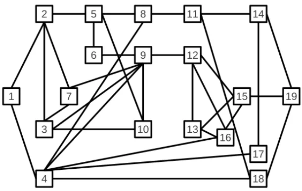
Numerical tests were performed to analyze the numerical behavior of the proposed algorithm and the influence of the parameters on its performance. Three different network topologies were used for the computational tests: the C-NET introduced in [24]; the RING introduced in [11]; and the NTS100 generated using a special program driver [6, 7]. For the sake of illustration, Figure 2 and 3 present the topologies of networks C-NET and NTS100, respectively. Table 1 gives the main characteristics of the three networks used in our numerical experiments. Given a root node

r, the hop-depth of a nodei ∈V \ {r}is the number of arcs in the path betweenrandi that has minimum length. The hop-based diameter of the graph is the largest hop-depth among the nodes of the network. C-NET and RING are full duplex networks,i.e., flow can be sent between two nodes in both directions and simultaneously.

Two sets of tests were made with these topologies:

– The first set concerns the C-NET network [24]. The aim is to verify the influence of the traffic throughput increase and the capacity expansion factor(c1e/c0e)on the number of

(10)

– The second test set was performed on the other two topologies RING and NTS100. The aim is to assess the effectiveness of the proposed implicit enumeration algorithm to solve the capacity expansion problem with different scenarios of larger networks and heteroge-neous traffic requirement demands.

The computation of the lower bound was performed by a specialized Flow Deviation algorithm for the convex multicommodity flow problem. That algorithm has been shown to be efficient since the early work of Frattaet al.[9], but it is generally known to become very slow when the algorithm approaches the optimal solution (see [3] for instance). To accelerate its convergence, a parallel tangent procedure (PARTAN, see [8]) was introduced in the direction finding step. The algorithm was coded in C.

Figure 2– The C-NET network with 19 nodes and 34 arcs.

Table 1– Characteristics of the test networks.

Network

nodes arcs OD-pairs aver. node hop-based

ID degree diameter

n m K 2m/n

C-NET 19 34 38 3.36 4

RING 32 60 496 3.75 6

NTS100 100 187 2000 3.74 11

The following notations were used:

• φ∗is the global optimal value;

• ¨φoptimal value of the convexified problem;

(11)

Figure 3– NTS100 network topology.

• φBar onis the solution obtained with BARON [27];

• φL Gis the solution obtained with LINDOGlobal [5, 17];

• Nggois the number of partial solutions enumerated to guarantee the global optimality;

• Nois the number of partial solutions enumerated until the optimal solution is found be not

necessarily proven to be optimal;

• NBar onis the number of visited nodes made by the Baron solver;

• NL Gis the number of visited nodes made by the LINDOGlobal solver;

• α= φ_¨∗ φ;

• αpg= φpg_φ_¨ .

4.1 First test set

In these experiments, the congestion cost is derived from the Kleinrock’s average delay function for M/M/1 queueing networks and defined byρ xe

ce−xe. We fixρ =1, see [11]. All arcs have the same initial capacity. And the expansion costπ1e, for each arce∈ E, is given, for each value of

the parameterγ = γ0e_c

0e equal to 0.7 and 0.9, by

π₁e=ργc0e

(c1e−c0e)

(12)

Tables 2 to 5 present the results for the C-NET network varying traffic requirement demands, parameterγand the available capacity for expansion.

The results show that the algorithm is rather sensitive to the capacity expansion factor. When

c1e = 4c0ethe number of iterations increase significantly, as observed for NggoandNoin

Ta-bles 4 and 5 in contrast withNggoandNoin Tables 2 and 3. Increasingγ affects the efficiency

of the algorithm. Both effects can be illustrated by the values ofαandαpg.

Table 2– Network C-NET, problem D38510.70.

¨

φ φ∗ φpg α αpg Nggo No Demand

13.64 13.75 13.86 1.01 1.01 26 24 0.50

37.68 39.21 39.43 1.04 1.05 206 178 1.00

68.78 70.59 71.54 1.02 1.04 152 66 1.50

181.94 184.19 184.99 1.01 1.02 146 110 2.00

Number of commodities 38,c0=5,c1=10,γ=0.70.

¨

13.64 13.75 13.86 1.01 1.02 0 0 0.50

56.45 56.91 59.67 1.01 1.06 18 16 1.00

135.06 140.21 144.10 1.04 1.07 92 27 1.50

291.38 301.38 304.86 1.03 1.05 208 112 2.00

¨

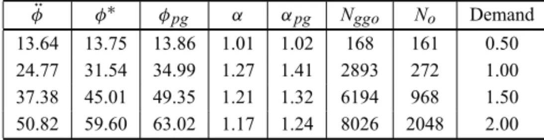
13.64 13.75 13.86 1.01 1.02 168 161 0.50

24.77 31.54 34.99 1.27 1.41 2893 272 1.00

37.38 45.01 49.35 1.21 1.32 6194 968 1.50

50.82 59.60 63.02 1.17 1.24 8026 2048 2.00

¨

13.64 13.75 13.86 1.01 1.02 4 2 0.50

42.05 49.31 54.41 1.19 1.29 286 268 1.00

75.52 95.14 112.54 1.26 1.49 2672 2248 1.50

110.08 133.57 151.42 1.22 1.37 2944 317 2.00

(13)

the biggest is the number of solutions enumerated. Observe that the global optimal solution was reached in many instances, some of them well beforeNggo≫No.

Table 6 shows the results obtained solving the mixed integer nonlinear formulation of the prob-lem (DCE) using two commercial solvers: BARON and LINDOGlobal [5, 17] and the results of the proposed algorithm. The Baron and the LINDOGlobal solvers were not able to guarantee the optimality of the results within the adopted time limits and or the number of iterations limits. They were not able to obtain the guaranteed global optimum of the C-NET problem. The LIN-DOGlobal solver uses linear approximations of the original problem which explains the large number of iterations within the limits of runtime.

Table 6– Network C-NET, continuousversusdiscrete formulations results.

c₀ c₁ γ φ¨ φ∗ φBar on φL G Nggo NBar on NL G Demand

5 10 0.70 13.64 13.75 13.75 13.75 26 1000 16744566 0.50

5 10 0.70 37.68 39.21 39.61 40.45 206 1000 8920413 1.00

5 10 0.70 68.78 70.59 70.60 71.50 152 1000 12103300 1.50

5 10 0.70 181.94 184.19 186.54 186.77 146 1000 8069258 2.00

5 10 0.90 13.64 13.75 13.75 13.75 0 1000 16890727 0.50

5 10 0.90 56.45 56.91 56.91 57.80 18 1000 8103096 1.00

5 10 0.90 135.06 140.21 140.21 140.21 92 1000 12034430 1.50

5 10 0.90 291.38 301.38 301.82 312.33 208 1000 8303808 2.00

5 20 0.70 13.64 13.75 13.75 13.75 168 10000 14855559 0.50

5 20 0.70 24.77 31.54 31.54 34.35 2893 10000 5799308 1.00

5 20 0.70 37.38 45.01 45.01 47.07 6194 10000 6564114 1.50

5 20 0.70 50.82 59.60 59.60 62.03 8026 10000 8239060 2.00

5 20 0.90 13.64 13.75 13.75 13.75 4 10000 16982685 0.50

5 20 0.90 42.05 49.31 49.31 57.20 286 (7200s) 6236884 1.00

5 20 0.90 75.52 95.14 101.01 127.01 2672 (7200s) 5670491 1.50

5 20 0.90 110.08 133.57 133.57 151.41 2944 (7200s) 7664995 2.00

For the problems withc1=10,NBar on≤1000, for the problems withc1=20,NBar on≤10000.

Maximum time available to solve the problems using BARON was 7200 seconds, and using LINDOGlobal was 4000 seconds.

All problems were solved in less than 3600 seconds using the proposed algorithm.

4.2 Second set of tests

The second set of tests concern the RING and the NTS100 topologies with heterogeneous traffic requirement demands. The congestion costs, as in the precedent set of experiments, is given by ρ xe

ce−xe. The following scheme was adopted for all these experiments:

– An initial feasible solution is computed using algorithms proposed in [7].

(14)

• In a first set of instances, the demand is uniformly multiplied by a throughput factor of 20%, 40%, 60%, 80% and 100% until capacity expansion becomes economically interest-ing.

– In the second set, the demand increase is no more uniform: half of the demands receive the same throughput factor, but 25% receive 50% more, and 25% receive 25% less. The results are exposed in Tables 8 to 11.

– An initial distribution of the increase of demand between the OD-pairs was defined ran-domly and fixed for each instance.

– The parameterρused to compute congestion costs is set to 500, 1000, 5000, and 10000.

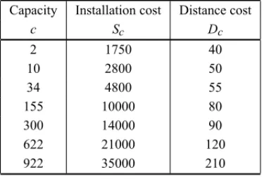
Table 7– Available capacities and costs.

Capacity Installation cost Distance cost

c Sc Dc

2 1750 40

10 2800 50

34 4800 55

155 10000 80

300 14000 90

622 21000 120

922 35000 210

πc=Sc+Dcti j.

A small number of iterations was needed to solve the proposed instances. Considering the com-plexity of the studied problem (CNET=234 =17,179,869,184 solutions, RING=260solutions, NTS100=2187solutions), one can evaluate the effectiveness of the proposed method. The sec-ond set of test problems was easier to be solved. This can be explained by noting that for these instances, the quality of the lower bound obtained by solving the problem with the convex enve-lope of the integrated function of congestion and expansion costs,c.f., Figure 1, is very good.

At each iteration of the implicit enumeration algorithm a convex multicommodity flow problem is solved. A convex multicommodity flow problem can be difficult, especially if feasibility prob-lems appear when an arc flow is close to the arc capacity. The decision to apply the Partan was primarily due to the gain in speed in solving problems is adequate for a precision of about 1% or better. Each multicommodity flow subproblem spent from a second fraction to several minutes.

(15)

Table 8– RING network and uniform demand increase.

ρ φ¨ φ

∗ _φ

pg

α αpg

Aver. increase

[$] ×106 [$] ×106 [$] ×106 of demand %

1000 3.69 3.71 3.71 1.00 1.00 10

1000 3.84 3.91 3.92 1.01 1.02 20

1000 4.05 4.11 4.15 1.01 1.02 40

1000 4.35 4.39 4.49 1.01 1.01 60

1000 4.70 4.76 4.76 1.01 1.01 80

1000 5.13 5.13 5.13 1.00 1.00 100

5000 4.22 4.26 4.26 1.01 1.01 10

5000 4.47 4.50 4.50 1.00 1.00 20

5000 4.79 4.84 4.84 1.01 1.01 40

5000 5.17 5.23 5.23 1.01 1.01 60

5000 5.62 5.68 5.69 1.01 1.01 80

5000 6.31 6.35 6.37 1.01 1.01 100

10000 4.61 4.62 4.62 1.00 1.00 10

10000 4.95 5.00 5.00 1.01 1.01 20

10000 5.36 5.42 5.42 1.01 1.01 40

10000 5.84 5.87 5.87 1.00 1.00 60

10000 6.38 6.42 6.42 1.00 1.00 80

10000 7.03 7.08 7.10 1.01 1.01 100

Table 9– RING network and heterogeneous demand increase.

ρ φ¨ φ

∗ _φ

pg

α αpg No Nggo Aver. increase

[$] ×106 [$] ×106 [$] ×106 of demand %

500 3.70 3.82 3.85 1.01 1.02 32 138 25

500 4.06 4.14 4.27 1.025 1.05 84 98 50

500 4.88 4.93 4.93 1.01 1.00 2 4 100

1000 3.89 3.97 3.97 1.01 1.02 4 265 25

1000 4.21 4.33 4.33 1.01 1.02 1 2 50

1000 5.08 5.12 5.13 1.00 1.01 1 2 100

5000 4.01 4.02 4.03 1.01 1.00 5 555 25

5000 4.97 5.02 5.02 1.01 1.01 1 2 50

5000 6.30 6.37 6.37 1.01 1.01 1 2 100

10000 4.87 4.91 4.92 1.01 1.01 6 365 25

10000 5.59 5.64 5.64 1.01 1.01 3 1 50

10000 7.06 7.07 7.07 1.00 1.01 5 1 100

(16)

Table 10– RING network and heterogeneous demand increase.

ρ No Nggo Aver. increase

of demand %

500 32 138 25

500 84 98 50

500 2 4 100

1000 4 265 25

1000 1 2 50

1000 1 2 100

5000 5 555 25

5000 1 2 50

5000 1 2 100

10000 6 365 25

10000 3 1 50

10000 5 1 100

Table 11– NTS100 network and heterogeneous demand increase.

ρ φ¨ φ

∗ _φ

pg

α αpg No Nggo

Aver. increase

[$] ×106 [$] ×106 [$] ×106 of demand %

500 3.70 3.82 3.85 1.01 1.02 32 138 25

500 4.06 4.14 4.27 1.025 1.05 84 98 50

500 4.88 4.93 4.93 1.01 1.00 2 4 100

1000 3.89 3.97 3.97 1.01 1.02 4 265 25

1000 4.21 4.33 4.33 1.01 1.02 1 2 50

1000 5.08 5.12 5.13 1.00 1.01 1 2 100

5000 4.01 4.02 4.03 1.01 1.00 5 555 25

5000 4.97 5.02 5.02 1.01 1.01 1 2 50

5000 6.30 6.37 6.37 1.01 1.01 1 2 100

10000 4.87 4.91 4.92 1.01 1.01 6 365 25

10000 5.59 5.64 5.64 1.01 1.01 3 1 50

10000 7.06 7.07 7.07 1.00 1.01 5 1 100

5 CONCLUSION

(17)

The literature has scarce approaches to find exact solution of the discrete capacity expansion and flow assignment problem. Basically two lines of approaches have been adopted: Benders decomposition [20] and methods based on difference of convex functions – DC programming [21]. Recently a conic quadratic formulation was proposed [26]. The results show that the implicit enumeration algorithm proposed here can be considered as an alternative available to solve to global optimality such large scale problems.

Future research is to be done on the extension of the proposed approach to deal with multiple choices of available capacities for expansion on each arc. It remains to show that lower bounds obtained with the convex envelope of the integrated function of expansion and congestion costs remain sharp in the presence of multiple expansions.

ACKNOWLEDGMENTS

This work has been supported by CNPQ (305164/2010-4) and (473763/2011-7).

REFERENCES

[1] BALASE. 1965. An additive algorithm for solving linear programs with zero-one variables. Opera-tions Research,13: 517–546.

[2] BALASE. 1966. Discrete programming by the filter method.Operations Research,13: 915–955. [3] BERTSEKASDP & GALLAGERRG. 1987. Data Networks, Prentice-Hall.

[4] DECAMARGORS, MIRANDAJRG, FERREIRARPM & LUNAHP. 2009. Multiple allocation hub-and-spoke network design under hub congestion.Computers and Operations Research,36: 3097– 3106.

[5] CZYZYKJ, MESNIERM & MORJ. 1998. The NEOS Server.IEEE Journal on Computational Sci-ence and Engineering, vol. 5.

[6] DOARMB & NEXIONA. 1996. A better model for generating test networks.Proceedings of Globe-com ’96, pp. 86–93.

[7] FERREIRARPM & LUNAHPL. 2003. Discrete capacity and flow assignment algorithms with per-formance guarantee.Computer Communications,26: 1056–1069.

[8] FLORIANM, GULATJ & SPIESSH. 1987. An efficient implementation of the PARTAN variant of the linear approximation method for the network equilibrium problem.Networks,17: 319–339. [9] FRATTAL, GERLAM & KLEINROCKL. 1973. The flow deviation method: an approach to

store-and-forward communication network design.Networks,3: 97–133. [10] www.gams.com, consulted on september 19, 2012.

[11] GAVISHB & NEUMANNI. 1989. System for routing and capacity assignment in computer commu-nication networks.IEEE Transactions on Communications,37: 360–366.

[12] GAVISHB & ALTINKEMERK. 1990. Backbone network design tools with economic tradeoffs.ORSA Journal on Computing,2: 236–252.

(18)

[14] GERLA M & KLEINROCKL. 1977. On the topological design of distributed computer networks.

IEEE Transactions on Communications,25: 48–60.

[15] GERLAM, MONTEIROJAS & PAZOSR. 1989. Topology design and bandwith allocation in ATM nets.IEEE Journal on Selected Areas in Communications,7: 1253–1261.

[16] GLOVERF. 1965. A multiphase-dual algorithm for the zero-one integer programming problem. Op-erations Research,13: 879–919.

[17] GROPPW & MORE´J. 1997. Optimization Environments and the NEOS Server.Approximation The-ory and Optimization, M.D. Buhmann and A. Iserles, eds., pp. 167–182, Cambridge University Press. [18] ISHFAQ R & SOX C. 2012. Design of intermodal logistics networks with hub delays. European

Journal of Operational Research,220: 629–641.

[19] LUNA HPL & MAHEY P. 2000. Bounds for global optimization of capacity expansion and flow assignment problems.Operations Research Letters,26: 211–216.

[20] MAHEYP, BENCHAKROUNA & BOYERF. 2001. Capacity and flow assignment of data networks by generalized Benders decomposition.J. of Global Optimization,20: 173–193.

[21] MAHEYP, PHONG TQ & LUNA HPL. 2001. Separable Convexification and DC Techniques for Capacity and Flow Assignment Problems.RAIRO Operations Research,35: 269–281.

[22] MAHEYP & SOUZA MC. 2007. Local optimality conditions for multicommodity flow problems with separable piecewise convex costs.Operations Research Letters,35: 221–226.

[23] MORABITOR &DESOUZAMC. 2010. Roteamento de multi-fluxos em redes de filas genericas.

Pesquisa Operacional,30: 583–600.

[24] OUOROUA, MAHEYP & VIALJP. 2000. A survey of algorithms for convex multicommodity flow problems.Management Science,46: 126–147.

[25] SOUZAMC, MAHEYP & GENDRONP. 2008. Cycle-based algorithms for multicommodity network flow problems with separable piecewise convex costs.Networks,51: 133–141.

[26] SINANG. 2011. A conic quadratic formulation for a class of convex congestion functions in network flow problems.European Journal of Operational Research,211: 252–262.