Braz. J. Chem. Eng. vol.32 número1

ISSN 0104-6632 Printed in Brazil

www.abeq.org.br/bjche

Vol. 32, No. 01, pp. 293 - 302, January - March, 2015 dx.doi.org/10.1590/0104-6632.20150321s00001653

Brazilian Journal

of Chemical

Engineering

STEADY

STATE

AND

PSEUDO-TRANSIENT

ELECTRIC

POTENTIAL

USING

THE

POISSON-BOLTZMANN

EQUATION

L. C. dos Santos

1,2

, F. W. Tavares

2,3*

, A. R. Secchi

2

, E. C. Biscaia Jr.

2

and V. R. R. Ahón

4 1

Petrobras, Centro de Pesquisas e Desenvolvimento (CENPES), Av. Horácio Macedo 950, CEP: 21941-915, Rio de Janeiro - RJ, Brazil.

E-mail: leticiacotia@hotmail.com

2_{COPPE, Programa de Engenharia Química, Universidade Federal do Rio de Janeiro,} Av. Horácio Macedo 2030, CEP: 21945-970, Rio de Janeiro - RJ, Brazil.

Phone: + (55) (21) 2562-7650 *

E-mail: tavares@eq.ufrj.br ; arge@peq.coppe.ufrj.br; evaristo@peq.coppe.ufrj.br 3

Escola de Química, Universidade Federal do Rio de Janeiro, Av. Horácio Macedo 2030, CEP: 21945-970, Rio de Janeiro - RJ, Brazil.

4

Departamento de Engenharia Química e de Petróleo, Universidade Federal Fluminense, Rua Passo da Pátria, 156, CEP: 24210-240, Niterói - RJ, Brazil.

E-mail: ruiz@vm.uff.br

(Submitted: January 31, 2012 ; Revised: April 29, 2014 ; Accepted: April 29, 2014)

Abstract - A method for analysis of the electric potential profile in saline solutions was developed for

systems with one or two infinite flat plates. A modified Poisson-Boltzmann equation, taking into account non-electrostatic interactions between ions and surfaces, was used. To solve the stated problem in the steady-state approach the finite-difference method was used. For the formulated pseudo-transient problem, we solved the set of ordinary differential equations generated from the algebraic equations of the stationary case. A case study was also carried out in relation to temperature, solution concentration, surface charge and salt-type. The results were validated by the stationary problem solution, which had also been used to verify the ionic specificity for different salts. The pseudo-transient approach allowed a better understanding of the dynamic behavior of the ion-concentration profile and other properties due to the surface charge variation.

Keywords: Electric Potential; Poisson-Boltzmann; Finite Difference.

INTRODUCTION

At the interface of the disperse and the dispersant phases of a colloidal system there are characteristic surface phenomena, like adsorption effects and an electric double layer that are very important to de-termine the physicochemical properties of the whole system (Lima et al., 2008). In the classical approach, the Poisson-Boltzmann (PB) equation does not take into account the non-electrostatic interactions present between ions and surfaces. However, the modified PB equation used in this study enables the ionic

specificity to be described, as verified in several colloidal systems.

method to show the behavior of ions close to elec-trodes with changinged potential. Although a very good numerical technique was used, Shestakov et al. (2002) reported results that are limited for general electrolytes. The authors did not include ionic speci-ficity (Hofmeister effect). Here, we include the dis-persion interaction between each ion and the elec-trode wall (from Lifshitz theory as described in Ninham and Yaminsky, 1997) to take into account the differ-ence between salt types. The Hamaker potentials are obtained elsewhere (Tavares et al., 2004, Livia et al., 2007).

The PB equation in 1-D form is a second order non-linear ordinary differential equation with Dirichlet and/or Neumann boundaries conditions. An analyti-cal solution for this equation is only available for particular cases like when the system is composed of a single plate and the classical PB approach for symmetrical electrolyte solution is used (Lima et al., 2007). In this study, the PB equation was solved for the classic and modified forms, for one or two flat plate systems, using the finite-difference method and a numeric approach, which is detailed in the second and third section of this paper. A pseudo-transient form of this equation is described in the fourth sec-tion. Finally, results and conclusions are presented in the last sections.

POISSON-BOLTZMANN EQUATION

In a liquid medium with electric charges, the ba-sic form of the Laplace equation gives place to the Poisson equation, shown in Equation (1), which re-lates the vector field divergence to the charge den-sity,



(Equation (2)).

 





 

0 w x x

      (1)

( ) _{i i}( )

i

x e



z c x

 (2)

in which c_i is the concentration of ion i, e is the ele-mentary charge, z_i is the valence of ion i, ₀ the vac-uum permittivity, and _w the water dielectric con-stant (Lima et al., 2007).

From the chemical potential of each ion in solu-tion, the Boltzmann distribution (Equation (3)) of the ions can be obtained.

0

( )

( ) exp i io

i i

B

E x E

c x c

k T

  

 _ _

  (3)

where c_i0 is the concentration of ion i in the bulk so-lution, E_i0is the reference state potential energy for ion i, and E_i is the potential energy of ion i defined as the sum of the electrostatic potentials plus the dispersion interactions (U_i) between the ion

i

and the surface (non-electrostatic potentials). Considering that all potentials between ions and macro particles in an aqueous solution go asymptotically to zero in the bulk phase (x  E_i0 0, i), Equation (3) becomes:

( ) ( )

( ) exp i i

i io

B

z e x U x

c x c

k T

  

 _ _

 



(4)

Substituting Equation (4) in (2), gives (Equation (5)):

 

( ) ( )

exp i i

i io

B

z e x U x

x e z c

k T

  

 _ _

 





 (5)

Substituting Equation (5) into Equation (1), gives the second-order non-linear modified PB equation:

 





0

( ) ( )

exp i i 0

w i io

B

z e x U x

x e z c

k T

  

   _ _

 





   (6)

NUMERICAL SOLUTION OF THE POISSON-BOLTZMANN EQUATION

This section presents a pseudo-transient approach to calculate the electrical potential profile using a modified Poisson-Boltzmann equation in different conditions. The profile trends presented in the Re-sults section, based on the data calculated from this approach, in some cases are all well known; how-ever, these trends are confirmed and presented in a different way using 3D figures.

Two kinds of geometry have been studied. The problem domains for each case are:

ion

r   x for one flat plate

ion

ion x L r

r    for two parallel plates

in which r_ion is the ionic radius (here all ions have the same size), xis the independent variable and Lis the distance between the two flat plates.

The Boundary Conditions

isoelec-tric point and, ii) Systems with a non-charged sur-face, such as the air/water interface. For an infinite flat plate, the first boundary condition (BC), valid for both systems (Equation (7)), admits that the electric field goes asymptotically to zero in the bulk phase (x ). Applying Gauss’ law for charged surfaces, the second BC (Equation (8)) comes from the elec-tric field generated by the surface charge density,



(Moreira et al., 2007):

 

lim 0

x

x

  (7)

 

0

ion w

x r

d x

dx _  

 

  (8)

Equation (8) is also used for non-charged sur-faces, at which  0.

In the case of two parallel infinite flat plates, the first BC (Equation (9)) for both systems admits that the electric field profile has a symmetry condition in the mid-point of the domain (xL/ 2).

 

/2

0

x L

d x

dx _ 



(9)

The second BC is also represented by Equation (8).

One Infinite Flat Plate – Dimensionless Form

For both geometries studied, the corresponding model equations were rewritten in dimensionless form in order to avoid scaling problems during the numerical resolution.

Defining the new independent variable y:

exp( )

y kx 0 y exp(kr_ion) (10)

The Debye-Length (k1) is defined by:

2 2

0 2

i i i o w B

e z c

k

k T





  (11)

In which k_B is the Boltzmann constant and Tis the temperature.

The new dependent variable (dimensionless elec-tric potential) is defined as:

 

 

B

e y

y

k T

 

 (12)

and the ionic strength of the solution, is given by:

2

1

2 _i i io

I 



z c (13)

The dispersion interaction between each ion and the flat surface, in the Hamaker approach, is given by (Israellachvili, 1995):

 

 

3

3 3

1 /

ln

  

i i i B

B B

U x H H k k T

k T k T x y

(14)

in which H_i is the dispersion coefficient, estimated here by the Lifshitz theory (for van der Waals interactions) (Israellachvili, 1995). Its dimensionless form, H_i*is defined by:

3

* i

i B

H k H

k T

 (15)

For this geometry, the modified dimensionless form of the PB equation is given by:

 

2

2 2

*

0 ₃

( ) ( )

1

exp 0

2 ln( )

i

i i i

i

d y d y

y y

dy dy

H

z c z y

I y



 

 _  _

 

 



 



(16)

And the two dimensionless BC are represented by Equations (17) and (18):

 

₀ 0

y

y

 

 (17)

 

exp( _ion) 2

y k r

d y k

y

dy _{ }  e I

 

(18)

Two Parallel Flat Plates – Dimensionless Form

In the case of two parallel flat plates, a similar procedure was performed; however, the independent variable was defined as:

ykx  kr_ion y k L



r_ion



(19)

 

2 *

0

2 3

( ) 1

exp 0

2

i

i i i

i

d y H

z c z y

I dy y    _  _    



 _ (20)

And the two dimensionless BC are represented by Equations (21) and (22):

 

0

2



kL

y dy y d



(21)

 

2 ion

y k r

d y k

dy _   e I

 

(22)

The Finite-Difference Method

As already mentioned, for the examples studied here, there are no analytical solutions. Therefore, the finite-difference method with second-order approxi-mations and n _{equally-spaced discretization}

inter-vals was used to solve the problem. The equations used to calculate the derivative at the domain end-points were generated from linear interpolation in

0 1

y  y y and y_n1 y y_n, respectively.

a) One Infinite Flat Plate – Steady State Condition

Applying the finite-difference method in Equations (16)-(18) (j1,2,...,n1) gives:

00

 (23)









 

 

2

1 1 1 1

* 0 ₃ * 0 ₃ 0 2 2 exp ln 1 exp 2 ln                        _{ }  _  _{ }         _  _     

j j j j j

j j j j j j H

z c z

y

H

z c z

I y        (24) 2 1 1 3 2

2 2 n n 2 n

k

Ine  

 

_   _

 

 _{  }

(25)

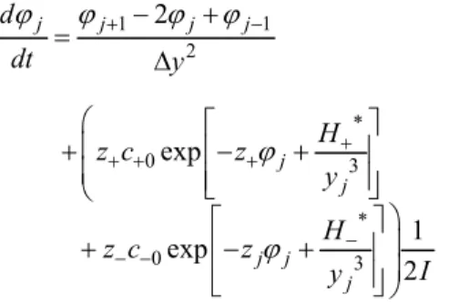
b) One Infinite Flat Plate – Pseudo-Transient Condition

To verify the effects on the electric potential pro-files, caused by changes in surface charge, a pseudo-transient model of the modified PB was proposed.

The pseudo-transient form of the modified PB equa-tion is an extension form of Shestakov et al. (2002). Furthermore, verifying these changes, it was possible to corroborate the results found with the steady-state problem solution. The pseudo-transient problem was formulated by defining a dimensionless potential variation with respect to a dimensionless time, t

(Shestakov et al., 2002). The system of n+1 alge-braic equations, generated in the previous item, is turned into a system with two algebraic equations defined by the boundary conditions (Equations (23) and (25)), and n-1 differential Equations (24) for the internal points (j1,2,...,n1).









 

 

2

1 1 1 1

* 0 ₃ * 0 ₃ 2 2 exp ln 1 exp 2 ln                        _{ }  _  _{ }         _  _      j

j j j j j

j j j j d j j dt H

z c z

y

H

z c z

I y         (26)

c) Two Parallel Plates – Steady-State Condition

Applying the finite-difference method in Equations (20)-(22) (j1,2,...,n1) gives:

0 1 2

4 1

3 3 3

k y eI



  

   (27)

1 1 2 * 0 ₃ * 0 3 2 0 exp exp                       _{ }              

j j j

j j j j j y H

z c z

y

H

z c z

y      (28) 2 1 1 4 3 3

n  n  n

   (29)

d) Two Parallel Plates – Pseudo-Transient Condition

1 1 2

*

0 3

*

0 ₃

2

exp

1 exp

2

 



  

  

 





  



   

 _{ }





 



   



 

 

j j j j

j j

j j j

d

dt y

H

z c z

y

H

z c z

I y

   





(30)

To solve item (b) and item (d), the initial condi-tions (j

 

0 ) are obtained from the solution of the

stationary problem for discharged surfaces.

To solve the proposed problem, a computational code was written in MATLAB, using internal solvers

like fsolve and ode45.

RESULTS AND DISCUSSION

To establish the mesh size, an analysis of the convergence of the electric potential on the surface as a function of n was performed. It was verified that, for above 100 intervals, the difference between the surface electric potentials was less than 104 _and

the electric potential value in the limit of x 

converged asymptotically to zero. To validate the implemented algorithm, we compared our results with those presented in the recent literature for NaCl, considering the dispersion interaction (Moreira et al., 2007). The base case was generated for NaCl solu-tions (1 M at 298.15K).

One Infinite Flat Plate – Steady State Condition

These results were generated for NaCl solutions (1 molar at 298.15 K). Figure 1 shows the electric potential profile generated by a discharged surface, Figure 2 (a) and (b) shows the electric potential pro-files for surfaces with positive and negative charges, respectively. From these results, it is possible to say that the modified PB equation accounts for the influ-ence of the non-electrostatic potential of each ion, that is, the ionic specificity given by the dynamic reorientation of the electronic cloud due to a nearby surface. This becomes evident in the electric poten-tial value observed on the surface, which is not zero even when the surface is not charged. The latter re-sult would not be obtained from the solution of the classical PB equation.

0 0.2 0.4 0.6 0.8 1 1.2 1.4 1.6 1.8 2

0 0.5 1 1.5 2 2.5 3

x(nm)

Ele

c

tric

P

o

te

n

tia

l

(m

V

)

Figure 1: Electric potential profile for a discharged

surface (Surface Charge Density =0 C/m2).

0 0.5 1 1.5 2

0 2 4 6 8 10

x(nm)

E

lect

ri

c P

o

te

n

ti

a

l (

m

V)

0 0.5 1 1.5 2

-3 -2.5 -2 -1.5 -1 -0.5 0 0.5

x(nm)

Ele

ctr

ic

Po

te

n

tia

l (

m

V

)

(a) (b)

Figure 2: (a) Electric potential profile for a positively charged surface (Surface Charge Density =0.012

One Infinite Flat Plate – Pseudo-Transient Condition

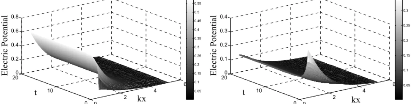
Results obtained from the dimensionless pseudo-transient model for one infinite flat plate are shown in Figures 3 and 4 (1 molar NaCl solutions at 298.15 K). Based on these results it is possible to verify changes in the electric potential profile caused by changes in the surface charge.

It is important to emphasize that the electric potential on the surface is not zero, even when the surface has no charge (see Figure 1). This is not true when using the classical PB equation, as can be seen in Figure 5.

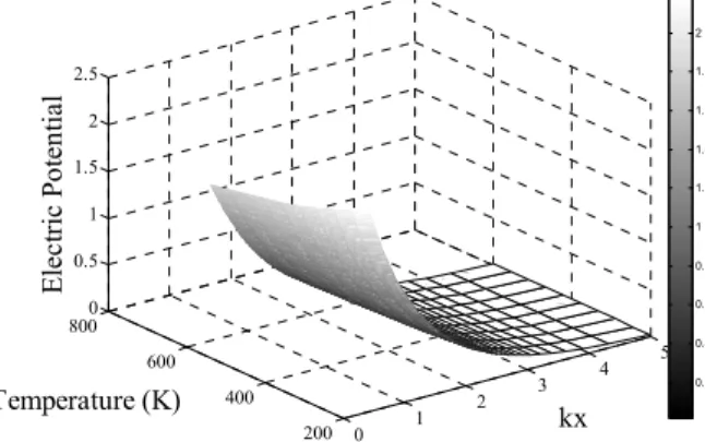
One Infinite Flat Plate – Case Study

Figures 6-10 show the electric potential profiles obtained by perturbations in the model parameters:

solution temperature, solution concentration, surface charge and the salt type. These results were obtained by evaluating the steady-state model for different parameter values. Regarding the solution tempera-ture, two opposite effects can be observed, a negative correlation (the potential decreases as the tempera-ture increases) when there is charge on the surface (Figure 6), and a positive one (Figure 7) when the surface is discharged. We show calculations for a very large range of temperature (from 200 to 600 K). At very high pressure (i.e., 109 Pa), water is an in-compressible liquid in this temperature range. Be-cause the calculations are carried out in the McMillan-Mayer framework, results are independent of pressure. Other important point is about the di-electric constant. The didi-electric constant decreases when temperature increases. However, we assume that the product  _{o w B}k T is independent of temperature.

0

2 4

6

0 10

20 0 0.2 0.4 0.6 0.8

kx t

E

lect

ri

c P

o

te

nt

ia

l

0.05 0.1 0.15 0.2 0.25 0.3 0.35 0.4 0.45 0.5 0.55

0 2

4

6

0 10

20 0 0.1 0.2 0.3 0.4

kx t

E

lect

ri

c P

o

te

nt

ia

l

0.05 0.1 0.15 0.2 0.25 0.3

Figure 3: Dimensionless electric potential profile

for increasing surface charge (initial=0 C/m2 and

final=0.012 C/m2).

Figure 4: Dimensionless electric potential profile

for decreasing surface charge (initial=0.012 C/m2 and final=0 C/m2).

0 2

4 6

0 10

20 -0.1 0 0.1 0.2

kx t

Ele

c

tric

P

o

te

n

tia

l

0.02 0.04 0.06 0.08 0.1 0.12 0.14 0.16 0.18

Figure 5: Dimensionless electric potential profile for decreasing surface charge (initial=0.012 C/m2 and

0 1 2 3 4 5 200 400 600 800 0 0.5 1 1.5 2 2.5 kx E le c tr ic P o te n tia l Temperature (K) 0.2 0.4 0.6 0.8 1 1.2 1.4 1.6 1.8 2 0 1 2 3 4 5 200 300 400 500 600 7000 0.02 0.04 0.06 0.08 0.1 0.12 kx Temperature (K) Ele ctr ic Po te n ti al 0.01 0.02 0.03 0.04 0.05 0.06 0.07 0.08 0.09 0.1 0.11

Figure 6: Dimensionless electric potential

pro-file for temperatures between 200 and 600 K with charged surface (Surface Charge Density =0.06 C/m2)

Figure 7: Dimensionless electric potential

pro-file for temperatures between 200 and 600 K for a discharged surface (Surface Charge Density =0 C/m2).

1 2 3 4 5 6 2 3 4 5 6 7 0 0.5 1 1.5 2 kx Concentration (M) E le ctr ic P o te nti al 0.2 0.4 0.6 0.8 1 1.2 1.4 1.6 1.8 2 2.2 0 1 2 3 4 5 6 -0.03 -0.02 -0.01 0 0.01 0.02 0.03-1 -0.5 0 0.5 1 kx harge Density (C/m2)

E lect ri c P o te nt ia l -0.6 -0.4 -0.2 0 0.2 0.4 0.6 0.8 1 Surface Charge

Density (C/m2₎ 0

1 2 3 4 5 6 -0.03 -0.02 -0.01 0 0.01 0.02 0.03-1 -0.5 0 0.5 1 kx harge Density (C/m2)

E lect ri c P o te nt ia l -0.6 -0.4 -0.2 0 0.2 0.4 0.6 0.8 1 Surface Charge

Density (C/m2₎

Figure 8: Dimensionless electric potential

pro-file for concentrations between 2 and 6 molar with a charged surface (Surface Charge Density =0.06 C/m2).

Figure 9: Dimensionless electric potential

profile for surface charge densities between: -0.024 and -0.024 C/m2.

Figures 6 - 9 were obtained for NaCl. The base case was done at 298 K and 1M. The results in Figures 10 (a) and (b) were obtained by evaluating the steady-state model for different salts (NaCl, KCl, BaCl2 and CaCl2) and concentration 1M. It is note-worthy that the ion specificity shown (Hofmeister effect) in Figure 10 (a) loses its influence in cases

where the surface charge is high. For these cases, electrostatic effects outweigh the others and the valence of the ions in solution becomes more relevant (Figure 10 (b)). In conclusion, in Figure 10 (b), it is not possible do distinguish NaCl and KCl. In addition, results obtained for BaCl2 and CaCl2 are praticaly the same.

0 1 2 3 4 5 6

0 0.02 0.04 0.06 0.08 0.1 0.12 0.14 kx E lect ri c P o te nt ia l NaCl KCl BaCl2 CaCl2

0 1 2 3 4 5 6

0 0.5 1 1.5 2 2.5 kx E lect ri c P o te nt ia l NaCl KCl BaCl2 CaCl2 (a) (b)

Two Parallel Plates – Steady-State Condition

These results were generated for NaCl solutions (1 molar at 298.15 K). Figures 11(a) and 11(b) show the results generated for the geometry with two charged parallel flat plates, where the influence of the distance (L) between the two plates on the electric potential profile can be seen.

A critical point was observed half way between the two plates; however, the potential value at this

point is not necessarily zero and it increases (in magnitude) as the plates come closer to each other.

Two Parallel Plates – Pseudo-Transient Condition

The results obtained from the dimensionless pseudo-transient model for this geometry are shown in Figures 12 and 13. Based on these results, it is possible to verify changes in the electric potential profile due to changes in the surface charge.

0 0.5 1 1.5 2 2.5 3 3.5

0 1 2 3 4 5 6 7

x(nm)

E

le

c

tr

ic

Po

te

n

tia

l (

m

V

)

0 0.5 1 1.5

0 1 2 3 4 5 6 7

x(nm)

Ele

ctric

P

o

te

n

tia

l (m

V

)

(a) (b)

Figure 11: (a) Electric potential profile with L 3.5 nm(Surface Charge Density =0.034 C/m2); (b) Electric potential profile with L1.5 nm (Surface Charge Density =0.034 C/m2).

0 2

4 6

0 5 10 15 20 -0.1 0 0.1 0.2 0.3 0.4 0.5 0.6

kx t

E

lec

tr

ic P

o

te

n

ti

al

0 0.05 0.1 0.15 0.2 0.25 0.3 0.35 0.4 0.45 0.5

El

ec

tr

ic

P

o

te

nt

ial

0 2

4 6

0 5 10 15 20 -0.1 0 0.1 0.2 0.3 0.4 0.5 0.6

kx t

E

lec

tr

ic P

o

te

n

ti

al

0 0.05 0.1 0.15 0.2 0.25 0.3 0.35 0.4 0.45 0.5

El

ec

tr

ic

P

o

te

nt

ial

Figure 12: Effect of inversion of the surface charge density () on the dimensionless electric potential

profile with L3 nm (initial=+0.024 C/m2 and final=-0.024 C/m2).

0 2

4 6

8 10

0 1 2 3 4 5 -1 -0.8 -0.6 -0.4 -0.2 0 0.2 0.4 0.6

kx t

E

lec

tr

ic Potenti

al

-0.8 -0.6 -0.4 -0.2 0 0.2 0.4

Two Parallel Flat Plates – Case Study

Figures 14-17 show the profiles obtained by changes in: solution temperature, solution concentra-tion, surface charge and type of salt used. Figures 14 - 16 were obtained for NaCl. The base case was done at 298 K and 1M. The results in Figure 17 were ob-tained by evaluating the steady-state model for dif-ferent salts (NaCl, KCl, BaCl2 and CaCl2) and con-centration 1M.

In a similar fashion, Figures 14, 15, 16 and 17 show the electric potential profiles obtained by changes in

solution temperature, solution concentration, surface charge, and type of salt used. The results show that the electric potential is not necessarily zero in the middle of the domain, only the critical point condi-tion is established by the problem boundary condicondi-tions. As shown in Figure 17, in cases where the surface charge is high, the influence of the electrostatic effects increases and the behavior of the physical properties is only modified by the valence of the ions present in the solution. Once more, in Figure 17, it is not possible to distinguish NaCl and KCl. Also, the results obtained for BaCl2 and CaCl2 are the same.

0 1

2 3

4 5

6 7

150 200 250 300 350 400 450 500 550 600 650

0 0.2 0.4 0.6 0.8 1

Temperature (K)

E

lect

ri

c P

o

ten

ti

al

0.1 0.2 0.3 0.4 0.5 0.6 0.7 0.8 0.9

kx

0 1

2 3

4 5

6 7

150 200 250 300 350 400 450 500 550 600 650

0 0.2 0.4 0.6 0.8 1

Temperature (K)

E

lect

ri

c P

o

ten

ti

al

0.1 0.2 0.3 0.4 0.5 0.6 0.7 0.8 0.9

kx

0 2

4 6

8 10 12

0.5 1

1.5 -0.4 -0.2 0 0.2 0.4 0.6

kx Concentration (M)

E

lec

tr

ic

P

o

tent

ial

-0.2 -0.1 0 0.1 0.2 0.3 0.4 0.5

Figure 14: Dimensionless electric potential profile

with temperatures between 200 and 600 K, with charged surface, andL3 nm (Surface Charge Den-sity =0.06 C/m2).

Figure 15: Dimensionless electric potential

pro-file for concentrations between 0.5 and 1.5 mo-lar, with charged surface and L3 nm (Surface Charge Density =0.06 C/m2).

0 1

2 3

4 5

6

-0.06 -0.04 -0.02 0 0.02 0.04 0.06-1.2

-1 -0.8 -0.6 -0.4 -0.2 0 0.2 0.4 0.6

kx Surface Charge Density (C/m2)

E

le

ctric

P

o

te

ntia

l

-1 -0.5 0 0.5

Figure 16: Dimensionless electric potential profile for surface charge density between -0.06 and 0.06

C/m2 (L2 nm).

0 2 4 6 8 10 12 14 16 -0.2

0 0.2 0.4 0.6 0.8 1 1.2

kx

Ele

c

tr

ic

P

o

te

n

ti

a

l

NaCl KCl CaCl2 BaCl2

CONCLUSIONS

A modified Poisson-Boltzmann equation, taking into account non-electrostatic interactions between ions and surfaces was used to describe salt concen-trations close to one or two infinite flat plates. To describe pseudo-transient behavior, a set of ordinary differential equations generated from algebraic equa-tions and written in dimensionless variables was solved. This procedure permitted obtaining the dy-namic behavior of the ion-concentration profile and other properties due to the surface charge variation.

The proposed method to solve the pseudo-transient Poisson-Boltzmann equation that accounted for salt type and divalent counterions can be used to describe electrochemical devices, such as electrodes with different surface-charge frequency. Sensitivity analysis was successfully carried out to verify the potential and ion concentrations close to the elec-trode in response to temperature, solution concentra-tion, salt type, and surface charge.

NOTATION

i

c _{ion concentration}

0

i

c _{concentration of ion}

_i

_{in the reference}

state (bulk phase)

i

E potential energy

io

E potential energy in the reference state (bulk phase)

i i

e z charge of each ion

H dispersion potential (Hamaker constant)

*

H dimensionless dispersion parameter

I ionic force in the bulk phase

i Counter

1

k Debye-Length

B

k _{Boltzmann constant}

L distance between two flat plates

ion

r radius of the ion

T temperature

t dimensionless time

U dispersion potential

x position coordinate, independent variable

y _{dimensionless independent variable} n number of discretization intervals

Z valence surface

y

 interval size

Greek Letters

 surface charge density

 dielectric constant

 _{charge volumetric density}  electric potential

 dimensionless electric potential

REFERENCES

Davis, M. E. and McCammon, J. A., Electrostatics in biomolecular structure and dynamics. Chem. Rev., 90, 509 (1990).

Honig, B. and Nicholls, A., Classical electrostatics in biology and chemistry. Science, 268, 1144 (1995). Israellchvili, J., Intermolecular and Surface Forces.

Second Edition. Academic Press, London (1995). Lima, E. R. A., Tavares, F. W., Biscaia Jr., E. C.,

Finite volume solution of the modified Poisson– Boltzmann equation for two colloidal particles. Physical Chemistry Chemical Physics, v. 9, pp. 3174-3180 (2007).

Lima, E. R. A., Horinek, D., Netz, R. R., Biscaia Jr., E. C., Tavares, F. W., Kunz, W., Boström, M., Specific ion adsorption and surface forces in col-loid science. Journal of Physical Chemistry B, v. 112, pp. 1580-1585 (2008).

Masliyah, J. H., Bhattacharjee, S., Electrokinetic and Colloid Transport Phenomena. John Wiley & Sons, Inc., Hoboken, New Jersey (2006).

Moreira, L. A., Bostrom, M., Ninham, B. W., Biscaia Jr., E. C., Tavares, F. W., Effect of the ion-protein dispersion interactions on the protein-surface and protein-protein interactions. J. Braz. Chem. Soc, v. 18, No. 1, pp. 223-230 (2007).

Ninham, B. W. and Yaminsky, V., Ion binding and ion specificity – The Hofmeister effect, Onsager and Lifschitz theories. Langmuir, 13, 2097-2108 (1997).

Tavares, F. W., Bratko, D., Blanch, H. and Prausnitz, J. M., Ion-specific effects in the colloid-colloid or protein-protein potential of mean force: Role of salt-macroion van der Waals interactions. J. Phys. Chem., B 108, 9228-9235 (2004).