TUNING OF TRANSIENT-EXCITED MUSICAL INSTRUMENTS
THROUGH OPTIMIZED STRUCTURAL MODIFICATION AND MODAL
TECHNIQUES
PACS 43.75M. Carvalho (1,2), V. Debut (1), J. Antunes (2)
(1) Instituto de Etnomusicologia - Centro de Estudos em M ´usica e Danc¸a, Faculdade de Ci ˆencias Sociais e Humanas, Universidade Nova de Lisboa, Av. de Berna, 26 C, 1069-061 Lisbon, Portugal. [email protected],[email protected]
(2) Centro de Ci ˆencias e Tecnologias Nucleares, Instituto Superior T ´ecnico, Universidade de Lisboa, Estrada Nacional 10, Km 139.7, 2695-066 Bobadela LRS, Portugal. [email protected]
Abstract
Tuning is a very important aspect for any musical instrument, not only concerning proper pitch but also the tonal quality of the instrument. In this paper, we address bar instruments as an application. Marimbas and vibraphones, have their first bending modes carefully tuned, being typically the first modal frequency ratios of 1:4:10. Such tuning is usually achieved by shaping the bar profiles with precision machine tools, a delicate and highly specialized task. In this paper we investigate the possibility of obtaining similar results using suitably designed tuning masses attached to the bars. Two application areas are illustrated: (1) Obtaining adequate tuning from common bars of constant cross-section loaded with masses; (2) Correcting badly tuned bars with a minimal set of loading masses. From a numerical point of view, such objectives are achieved by coupling structural modification techniques with effective optimization schemes. Two tuning approaches are proposed: the first one uses a full-sized finite element model of the mass-loaded bar, while the second one is based on a very effective reduced model built using the modes of the non-corrected bar. After presenting the developed tuning methods, we illustrate them on the above mentioned applications, based on simulated data. Validation experiments are currently being prepared.
1
Introduction
In this paper we couple optimization procedures with physical modeling techniques in order to explore a new method to tune vibraphone and marimba bars, by attaching suitably designed masses to them, a non-destructive, reversible and relatively effortless approach. Our method was drawn, essentially, to correct poorly tuned bars, with a minimal set of loading masses. With this in mind, we developed a methodology which consists in coupling structural modification techniques with effective optimization schemes, in order to predict the positions and weight of each mass, to comply with a pre-defined target of modal frequencies. Two approaches were used for the computations, the first using Finite Elements modeling (FEM) techniques coupled with optimization strategies, while the second is based in a modal formulation of the problem built from the modal properties of the unloaded bar calculated through FEM. For the bar modeling, a simple Euler-Bernoulli FEM beam model was used, although, the applied optimization techniques can be easily coupled with more refined models if needed.
For the optimization we use a gradient-based local optimization strategy which allows to find the minimum of a multivariable error-function. This optimization technique is fast, however, being gradient-based, it works only with continuous variables and it can get stuck in local minima, frequently being ineffective. For that reason, some strategies were developed in order to overcome these problems which will be discussed in this paper. After describing the physical modeling and the optimization strategies, we present some illustrative cases for which we apply these strategies to the tuning of vibraphone bars, in order to reach target frequencies complying the typical tuning ratios both for continuous and discrete mass variables. The numerical results demonstrate the feasibility of the developed method for the given conceptual system. The effectiveness and robustness of the proposed techniques illustrated by our simulations are quite encouraging. Experimental validation is currently being addressed.
2
Physical modeling
In order to predict the dynamical behavior of the system, two different approaches were used for the physical modeling of the bars, namely Finite Elements Method and modal formulation.
2.1
Finite Element Modeling
In this section we describe the FEM model for the original bar without the tuning masses referred to as the “original system” and the modeling of the system modified by additional masses attached to the bar - the “modified system”.
2.1.1 Original bar without masses
For the original system (i.e. the model of the bar without tuning masses), in order to study the lowest three flexural modes of interest, we used the Euler-Bernoulli beam model, which for a bar with variable cross-sectionBH(x)is formulated as [9]:
ρA(x)∂
2y
∂t2 + ∂2 ∂x2
EI(x)∂
2y
∂x2
= 0, (1)
whereρis the density of the bar material,A(x) =BH(x)is the cross-sectional area of the bar,yis the flexural movement,E is the Young modulus, and I(x) = BH12(x)3 is the bar flexural moment of inertia. Finite element discretization of Eq. (1) enables the computation of the elementary stiffness and mass matrices, which after assembling leads to the dynamical formulation of the bar in terms of the physical coordinates:
[Mos]{Y¨(t)}+ [Kos]{Y(t)}={0}. (2)
Here [Mos]and [Kos]are the global mass and stiffness matrices of the “original system” and {Y} is
frequenciesωmand modeshapes{ϕm}were computed assuming harmonic solutions:
{Y(t)}={ϕm}exp(iωmt), (3)
and solving the generalized eigenvalue problem with the classic formulation:
−ω2m[Mos] + [Kos]{ϕm}={0}. (4)
2.1.2 Bar with additional tuning masses
Modeling of the system modified by additional masses attached to the bar can be achieved in terms of the physical coordinates as:
[Mos]{Y¨(t)}+ [Kos]{Y(t)}=−[Mad]{Y¨(t)}, (5)
where[Mad]is the mass matrix of the additional point massesmpat p = 1, 2, ... , P locations, a diagonal
matrix with terms corresponding to the locations of the additional masses, whereMad(p, p) =mp. Thus,
from (5), we obtain the following formulation for the “modified system”:
[Mms]{Y¨(t)}+ [Kos]{Y(t)}={0}, (6)
where:
[Mms] = [Mos] + [Mad]. (7)
Similarly to the original system, the modal frequencies and corresponding modeshapes were computed through a generalized eigenvalue problem as described by:
−ω2m[Mms] + [Kos]
{ϕm}={0}. (8)
2.2
Modal-based modeling
A modal formulation of the system dynamics is surely well-suited for the aims of this work since it provides a physical model with a reduced number of equations and consequently requires less computational efforts.
2.2.1 Original bar without masses
To obtain the modal formulation for the basic system, we can reformulate (2) through the transformation:
{Y(t)}= [Φos]{Q(t)}, (9)
where[Φos] = [{ϕos1}{ϕos2}, ...,{ϕosn}]obtained in (4) andQ(t)is the vector of the modal amplitudes.
After multiplication by[Φos]T, and using the classical orthogonality properties, we obtain the following
modal formulation for the original system:
[Mos]{Q¨(t)}+ [Kos]{Q(t)}={0}, (10)
where:
[Mos] = [Φos]T[Mos][Φos] (11)
[Kos] = [Φos]T[Kos][Φos], (12)
are the diagonal modal mass and modal stiffness matrices of the original system. Moreover, in order to improve the results accuracy, the stiffness matrix[Kos]used for the computations was built as:
[Kos] = [Mos][ωexp2 ], (13)
being [ωexp2 ] = diag({ω12, ω22, ..., ω2n}), where ωn = 2πfn is the angular frequency of mode index n,
2.2.2 Bar with additional tuning masses
The modal formulation for the modified system can be obtained by applying the methodology described from (9) to (12) to the modal formulation of the modified system given in (6), thus resulting in:
[Mms]{Q¨(t)}+ [Kos]{Q(t)}={0}, (14)
where:
[Mms] = [Φms]T[Mms][Φms] = [Φms]T([Mos] + [Mad])[Φms] (15)
[Kms] = [Φms]T[Kos][Φms]. (16)
However, a clever and more economical solution for obtaining the modes of the mass-loaded system, most suitable for performing optimization iterations, may be devised directly from the modes of the original system. Starting from Eq. (5) and using Eq. (9), one obtains:
[Mos][Φos]{Q¨(t)}+ [Kos][Φos]{Q(t)}=−[Mad][Φos]{Q¨(t)}, (17)
hence, pre-multiplying by[Φos]T:
[Mos]{Q¨(t)}+ [Kos]{Q(t)}=−[Φos]T[Mad][Φos]{Q¨(t)}, (18)
obtaining:
[Mos] + [Φos]T[Mad][Φos]
{Q¨(t)}+ [Kos]{Q(t)}= 0 (19)
yielding to the modified eigenvalue problem for the mass-loaded system:
−ωm2 [Mos] + [Φos]T[Mad][Φos]
+ [Kos]
{ϕm}={0}. (20)
Notice that, because formulation (20) is already based on the reduced model of the original system, the computation of the mass-loaded modes using (20) is much more economical than the equivalent - but much larger - eigenvalue computation (8). Actually, an improvement of at least one order of magnitude in computation time is achieved when performing optimizations using the modal approach, comparing to the FEM.
3
Optimization strategies
Essentially, an optimization problem consists in finding the values of a set of variables that maximize or minimize an error-function. Most of the optimization problems can be formulated in several different manners using different strategies. In this study we used a deterministic local optimization method which proved to be effective [10]. Local optimization algorithms are gradient based and try to find the nearest local optimal solution. This is a fast method, but it is prone to get stuck in local minima. Therefore, some strategies were developed in order to avoid this problem. Moreover, being gradient based, it implies the use of continuous variables for the optimization. This allows accurate results, however, experimental work often becomes very costly and time consuming when working with continuous mass variables, since it would imply manufacturing n customized masses for each experiment. Then, for practical reasons, we also developed a discrete optimization strategy, in order to avoid the use of nonstandard mass devices for the experimental validation, which is now being prepared.
3.1
Continuous optimization
For the continuous optimization strategy our aim is to find the optimal mass values M∗
n =
{m∗
0 ≤ℓn ≤L) for a given numbernof masses required to minimize the differences between the actual
modal frequencies of the system and a given set of target frequencies. We used a multivariable function optimization approach in order to minimize the error-functionE(Mn, Ln):
E(Mn, Ln) = J
X
j=1
ωj⋆−ωj(Mn, Ln)
ωj⋆
, (21)
whereJ is the number of modes to optimize,ωj⋆ are the target frequencies, andωj(Mn, Ln)are the
computed modal frequencies for the mass valuesMn and their respective positionsLn. As mentioned
above, depending on the initial solution given, the algorithm tends to get trapped in a local minimum. In order to overcome this problem, we repeated the optimization process several times using random initial positions and mass values. Thus, several different initial solutions lead to several error values E(Mn, Ln). In the end, the minimal error valueE(Mn, Ln)gives the optimal solution (Mn∗, L∗n).
3.2
Discrete optimization
For the practical reasons mentioned above, we developed a discrete optimization strategy which combines continuous position variables Ln with a set of n predefined discrete mass values Md =
{md
1, md2, ..., mdN}, in order to find the discrete optimal solutionsM d n
∗
, with md
n ∈M d, and respective
positions that minimize (21). In this work we used a standard approach to solve discrete optimization problems, which consists in three basic steps [11]. First, a continuous optimization of the problem is performed in order to find the continuous optimal solution L∗
n andMn∗. Likely, the found continuous
mass values M∗
n do not belong to the predefined set of discrete possible mass values Md. Thus,
for each found M∗
n variable, the upper and lower closest discrete values belonging to Md are then
searched, thereby creating two possibilities for each variable. Secondly, for each possible set of discrete variables combination, a continuous optimization is performed in order to establish a new optimum value for the continuous position variablesL∗
n(Mnd). Finally, the comparison of the optimization
results for the several discrete value combinations allows us to find the optimal solution(L∗
n, Mnd
∗
)of the discrete problem.
4
Applications
In this section we illustrate the computations used in order to obtain typical vibraphone bar tuning ratios of 1:4:10 for the first three modes, having as starting point both an untuned vibraphone bar of variable cross section and a uniform cross section aluminium bar. In all cases, for the FEM modal computations, we used a mesh consisting of 64 elements and the values of 710 GPa and 2750 Kg/m3for the Young modulus and density, respectively.
4.1
Tuning a vibraphone bar
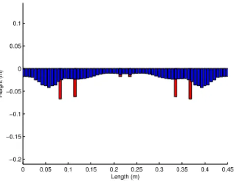
Here we present the optimization results for the tuning of a vibraphone bar of variable cross section, using the developed continuous and discrete optimization strategies previously described. The modeled bar dimensions are 0.45 m (length), 0.04 m (width) and variable heights between 1 and 0.042 m, with a total mass of about 1 Kg. The original fundamental frequency of the bar was of 271Hz (frequency of musical note C#), and tuning ratios 1:4.2:11.2 for the first three modes. In this case, the aim was to obtain the tuning ratios of 1:4:10, and 261Hz (frequency of musical note C) for the fundamental frequency, which corresponds to correct tuning modal errors of 4%, 8% and 14%, respectively.
4.1.1 Continuous optimization
0 0.05 0.1 0.15 0.2 0.25 0.3 0.35 0.4 0.45 −0.2
−0.15 −0.1 −0.05 0 0.05 0.1
Height (m)
Length (m)
Figure 1: FEM continuous optimization results (M∗
n, L∗n). Blue: original bar
profile; Red: additional tuning masses.
0 0.05 0.1 0.15 0.2 0.25 0.3 0.35 0.4 0.45
−0.2 −0.15 −0.1 −0.05 0 0.05 0.1
Height (m)
Length (m)
Figure 2: Modal continuous optimization results (M∗
n, L∗n). Blue: original bar
profile; Red: additional tuning masses.
0 5 10 15 20 25 30 35 40 0
0.01 0.02 0.03 0.04 0.05 0.06
Error
Iteration number
Figure 3: Error valueE(Mn, Ln).
Mass number
Optimal solution
FEM Modal
Continuous Discrete Continuous Discrete
L∗
n Mn∗ L∗n(M
d∗
n ) M
d∗
n L∗n Mn∗ L∗n(M
d∗
n ) M
d∗ n
1 0.091 0.116 0.098 0.110 0.082 0.084 0.083 0.090 2 0.105 0.066 0.107 0.060 0.115 0.086 0.113 0.090 3 0.198 0.013 0.205 0.010 0.215 0.009 0.206 0.010 4 0.252 0.013 0.245 0.010 0.235 0.009 0.244 0.010 5 0.345 0.066 0.343 0.060 0.335 0.086 0.337 0.090 6 0.359 0.116 0.352 0.110 0.368 0.084 0.366 0.090
Table 1: Computed Mass values and respective positions using the FEM and modal optimization approaches for both continuous and discrete optimization strategies.
and widths are the same as those of each element of the mesh (0.007m and 0.4m respectively), corresponding to the continuous optimal mass values M∗
n and positionsL∗n presented in Table 1, in
a total of 0.390 Kg and 0.358 Kg for the FEM and modal approaches respectively. As seen, different solutions were found for each approach, meaning the existence of several solutions that comply with the target tuning, and that different local minima were accepted as the solution for each case. Furthermore, Figure 3 displays a typical evolution of the error during the optimization process, illustrating the correct behavior of the optimization process.
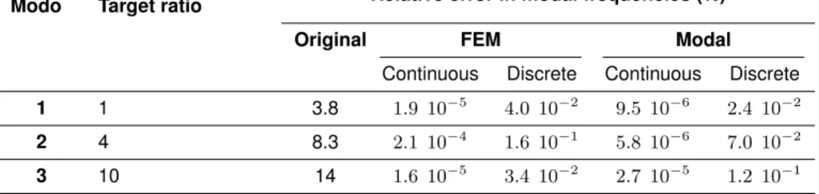
Modo Target ratio Relative error in modal frequencies (%)
Original FEM Modal
Continuous Discrete Continuous Discrete
1 1 3.8 1.9 10−5
4.0 10−2
9.5 10−6
2.4 10−2
2 4 8.3 2.1 10−4
1.6 10−1
5.8 10−6
7.0 10−2
3 10 14 1.6 10−5
3.4 10−2
2.7 10−5
1.2 10−1
Table 2: Modal errors for the first three modes, relative to the target frequency ratios of 1:4:10, using three different optimization approaches (continuous FEM, discrete FEM, continuous modal and discrete modal optimization).
before and after the optimizations. FEM and modal optimization approaches similarly provide results with great accuracy, illustrating the effectiveness of both developed approaches. However, the modal formulation allows faster computation times, since it is able to significantly reduce the number of equations needed to represent the system (in this case 7 equations).
4.1.2 Discrete optimization
We now turn to the results achieved through the discrete optimization strategy obtained using, initially, the respective continuous optimal solution (M∗
n, L∗n), presented in Section 3.1. In this case, we
predefined a set of discrete masses Md = {md
1, md2, ..., mdn}, in the range between 0 and 0.3 Kg,
with a step increase of 10 grams per mass, obtaining as optimal solution the discrete values Md n
∗
and respective positionsL∗
n presented in Table 1. By comparing the continuous and discrete optimal
solutions, we can see that the mass values of the continuous solution were rounded to the closest upper or lower mass values pertaining to the predefined set of discrete masses Md. Also, the continuous
optimal position solutionsL∗
nobtained with the continuous optimization strategy were slightly adjusted
in order to find the minimal errorE(Mn, Ln). In Table 2 we can see that the tuning errors are larger
than those obtained through the continuous optimization strategy as one would expect because of the limitations of the available masses. However, errors less than 1.6 10−1% still are very accurate results,
which would result in inaudible tuning errors.
4.2
Obtaining a vibraphone bar from an uniform bar
Here we illustrate the computations to obtain typical vibraphone bar tuning with ratios of 1:4:10 for the first three modes, having as starting point an uniform cross section alluminium bar with 0.5 m length, 0.06 m width and 0.02 m height and a mass of 1.8 Kg. The bar fundamental frequency is 412 Hz, and the original frequency ratios for the first three modes are 1:2.8:5.4. This corresponds to correct tuning errors of 106%, 42% and 11%, for the three modes of interest, which represents a far larger decrease of the modal frequencies than in sections 4.1.1 and 4.1.2.
4.2.1 Continuous optimization
The tuning masses and respective positions required to achieve the target tuning, given by the FEM and modal formulation optimization approaches are represented in Figures 4 and 5. In this cases, for representative purposes, we calculated the punctual tuning masses heights, assuming lengths of three times the length of a mesh element and widths equal to those of each element of the mesh and a density of 7850 Kg/m3(density of stainless steel). The corresponding continuous optimal mass valuesM∗
n and respective positionsL∗n are presented in Table 3. As expected, heavier masses were
0 0.05 0.1 0.15 0.2 0.25 0.3 0.35 0.4 0.45 0.5 −0.35
−0.3 −0.25 −0.2 −0.15 −0.1 −0.05 0
Height (m)
Length (m)
Figure 4: FEM continuous optimization results (M∗
n, L∗n). Blue: original bar
profile; Red: additional tuning masses.
0 0.05 0.1 0.15 0.2 0.25 0.3 0.35 0.4 0.45 0.5 −0.25
−0.2 −0.15 −0.1 −0.05 0 0.05 0.1
Height (m)
Length (m)
Figure 5: Modal continuous
optimization results (M∗
n, L∗n). Blue:
original bar profile; Red: additional tuning masses.
tuning. However, as we can see in Table 4, despite the large original mistuning, both FEM and modal approaches allow accurate results, demonstrating that the developed tuning approaches can be used not only for relatively small tuning corrections but also for substantial ones. Once again, different solutions, with total masses of 7.4 Kg and 5.0 Kg (for the FEM and modal approaches respectively) were found for each approach, which means that different local minima were accepted as the optimal solution for each case.
Mass number
Optimal solution
FEM Modal
Continuous Discrete Continuous Discrete
L∗
n Mn∗ L∗n(M
d∗
n ) M
d∗
n L∗n Mn∗ L∗n(M
d∗
n ) M
d∗ n
1 0.038 3.225 0.038 3.220 0.033 0.287 0.032 0.290 2 0.055 0.069 0.055 0.070 0.037 1.715 0.037 1.720 3 0.199 0.407 0.199 0.410 0.207 0.514 0.208 0.520 4 0.303 0.407 0.303 0.410 0.294 0.514 0.293 0.520 5 0.446 0.069 0.446 0.070 0.464 1.715 0.464 1.720 6 0.464 3.225 0.464 3.220 0.468 0.287 0.469 0.290
Table 3: Computed optimal mass values and respective positions using the FEM and modal approaches for both continuous and discrete optimization strategies.
Modo Target ratio Relative error in modal frequencies (%)
Original FEM Modal
Continuous Discrete Continuous Discrete
1 1 3.8 5.5 10−6
4.7 10−2
1.2 10−8
1.4 10−3
2 4 8.3 6.8 10−5
1.6 10−1
2.9 10−6
1.1 10−2
3 10 14 2.9 10−6
2.7 10−2
7.3 10−6
3.1 10−3
4.2.2 Discrete optimization
The discrete optimization strategy was performed starting from the FEM and modal continuous optimal solutions (M∗
n, L∗n)presented in Table 3 and predefining a set of discrete masses Md as in section
5.1.2, but this time for masses between 0 and 4 Kg. Also in this case, the tuning errors presented in Table 2 allow us to conclude that a very precise tuning can also be achieved with the discrete strategy.
5
Conclusions
In this work, we coupled physical modeling with optimization strategies in order to develop a methodology for the tuning of several transient-excited musical instruments. The methodology was illustrated with numerical calculations and the results show the effectiveness and robustness of the developed tuning techniques for two different conceptual cases. The use of gradient based local optimization methods, and particularly when combined with the modal formulation approach allows very fast computations. Being non-destructive and applicable to several musical instruments, we believe that these techniques can be very useful for musical instruments industry in the future. Experiments are being prepared in order to validate the presented tuning techniques.
References
[1] Bork, I., 1995. Practical Tuning of Xylophone Bars and Resonators.Applied Acoustics, 46, 103-127.
[2] Schoofs, A, Asperen, F., Maas P., and Lehr, A., 1987. A carillon of major-third bells: Computation of bell profiles using structural optimization.Music Perception, 4, 245-254.
[3] Kausel, W., 2001. Optimization of Brasswind Instruments and its Application in Bore Reconstruction.Journal of New Music Research, 30(1), 69-82.
[4] Debut, V., Kergomard, J. and Laloe, F., 2005. Analysis and optimization of the tuning of the twelfths for a clarinet resonator.Applied Acoustics, 365-409.
[5] Noreland, D., Kergomard, J., Lalo ¨e, F., Vergez, C., Guillemain, P. and Guilloteau, A., 2013. The logical clarinet: numerical optimization of the geometry of woodwind instruments. Acta Acustica united with Acustica, 99, 615-628.
[6] Carlsson, P. and Tinnsten, M., 2002. Numerical optimization of geometrical dimensions and determination of material parameters for violin tops. Forum Acusticum 2002, Sevilla, 16-20 September.
[7] Henrique L., and Antunes, J., 2003. Optimal Design and Physical Modelling of Mallet Percussion Instruments. Acta Acustica United With Acustica, 89, 948-963.
[8] Lambourg, C. and Chaigne, A., 2001. Time-domain simulation of damped impacted plates: Part 2 - Numerical model and results.Journal of the Acoustical Society of America, 109, 1433-1447.
[9] Inman, J., 2001. Engineering Vibration.Upper Saddle River, Prentice Hall.
[10] Gill, P., Murray, W. and Wright, M. 1981. Practical Optimization, London, Academic Press.
[11] Venkataraman, 2002. Applied Optimization with MATLAB Programming.John Wiley and Sons, New York.