Study of the influence of a DC electric field on the development of the embryo of the nematode Caenorhabditis elegans

(1)

Faculdade de Ciências

Departamento de Física

Study of the Influence of a DC Electric Field on the

Development of the Embryo of the Nematode

Caenorhabditis elegans

André de Albuquerque Rino Loureiro de Amorim

Dissertação

Mestrado Integrado em Engenharia Biomédica e Biofísica

Perfil em Engenharia Clínica e Instrumentação Médica

(2)

(3)

Faculdade de Ciências

Departamento de Física

Study of the Influence of a DC Electric Field on the

Development of the Embryo of the Nematode

Caenorhabditis elegans

André de Albuquerque Rino Loureiro de Amorim

Dissertação orientada por:

Prof. Dr. Philippe Renaud

École Polytechnique Fédérale de Lausanne Prof. Dr. Hugo Ferreira

Faculdade de Ciências da Universidade de Lisboa

Mestrado Integrado em Engenharia Biomédica e Biofísica

Perfil em Engenharia Clínica e Instrumentação Médica

(4)

(5)

(6)

(7)

List of Figures

Fig. 1.1: Galvani’s experiments using a frog leg preparation. The leg contracted when the cut end of the

sciatic nerve touched the leg muscle (1) or when the electrical discharge was applied directly to the nerve (2). When the surface of a section of the right sciatic nerve touched the intact surface of the left sciatic nerve, both legs contracted (3). (Image taken from [1]) ...2

Fig. 1.2: A stem cell divides asymmetrically originating two daughter cells with different fates. The

daughters may differentiate and proliferate or remain stem cells to divide asymmetrically again. A healthy tissue is composed by several differentiated cells. (Image taken from [6]) ...5

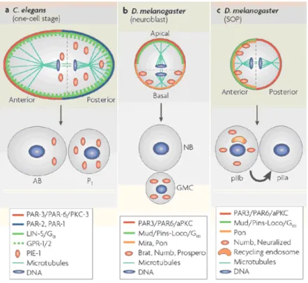
Fig. 1.3: Asymmetric division of the egg-cell of three different organisms. This is the first mitotic division

of embryogenesis. The polarized mother cell during anaphase is shown at the top of each panel, whereas the daughter cells that are produced by asymmetric division are shown at the bottom of each panel and are named below. The distribution of several components that are important for polarity establishment, spindle positioning and cell-fate determination is illustrated for the mother cell, and the distribution of cell-fate determinants is shown for daughter cells immediately after mitosis. Note that many of them are the same for the three organisms. Directional signalling between the anterior cell (pIIb) and the posterior cell (pIIa), whereby the Delta ligand from pIIb signals to the Notch receptor on pIIa, is denoted by a thick arrow in panel c. This is an example of an extrinsic mechanism of fate determination. (Image and

description taken from [8]) ...6

Fig. 1.4: Top: skin epithelium of the Xenopus embryo. The transepithelial potential results from active

transport and passive diffusion of ions across the basal and apical membranes of epithelial cells. Thigh junctions avoid the passage of ions outside the cells. Bottom left: wounding of an epithelial sheet (or localized disruption of tight junctions) creates a current leak at the wound site causing the immediate, catastrophic collapse of the TEP at the wound. The TEP is not affected distally, where the epithelial integrity and ion transport properties remain intact. Na+_{leak out the wound, resulting in an outward} injury current and a lateral voltage gradient (electric field) within the embryo (green arrows) oriented parallel to the epithelial sheet. The wound site is the cathode of the EF. Bottom right: circuit model of the wounded epithelium. Each battery represents the transepithelial potential for a patch of epithelium. It differs with the distance to the wound. Rw is the resistance of the wound, Rfluid is the resistance of the pound water where the frog embryo develops and Rtissue is the resistance of the tissue underlying the epithelium. (Image taken from [1]) ...8

Fig. 1.5: Orientation of the cleavage plane of transformed human corneal epithelial cells was affected by

applied EFs (strength and polarity as shown). (a) No field control. Cleavage furrows are evident and oriented randomly. (b) Dividing cells in an applied EF showed preferential orientation of the cleavage furrow. (Image and description taken from [10]) ...9

Fig. 3.1: Anatomy of an adult hermaphrodite C. elegans individual. A: DIC image of an adult

hermaphrodite. B: schematic drawing of its anatomical structures. (Image taken from [32]) ...14

Fig. 3.2: Life cycle of C. elegans at 22ºC. The time of fertilization is set to 0. Numbers in blue along the

(12)

40min after fertilization. Eggs are laid outside at about 150min after fertilization, during the gastrulation stage. The length of the animal at each pos-embryonic stage is marked next to the stage name in

micrometers. C. elegans embryogenesis will be presented in the next section. (Image and description taken from [32]) ...15

Fig. 3.3: DIC images of the larval stages of C. elegans. (Image taken from [32])...16

Fig. 3.4: C. elegans under microscope. The worm length is about 1mm. (Image taken from [48])...18

Fig. 3.5: Main stages of C. elegans embryogenesis. Cell names are written near the respective cells.

Anterior is left, ventral is down. a – d: 1-cell stage, showing the pro-nuclei and their migration. The oocyte pro-nucleus is signalled by (o) and the sperm pro-nucleus is signalled by (s). e: start of the first mitosis. f: 2-cell stage. g: 4-cell stage. h: 8-cell stage (one of the AB descendants is not visible. i: start of the gastrulation. j: comma stage. k: 1.5-fold (tadpole) stage. l: 3-fold (pretzel) stage. (Image taken from [54]) ...20

Fig. 3.6: Embryonic stages of development. The numbers below the horizontal axis show approximate

time in minutes after fertilization at 22ºC. The yellow bars indicate the period of time during which cells from a certain lineage migrate towards the inside of the embryo through the entry zone (the gastrulation cleft or ventral cleft) during gastrulation (blue bar). Red bar indicates elongation of the embryo that takes place between 400-640min due to circumferential contraction within the hypodermis. During elongation, the embryo becomes threefold thinner and its length increases about fourfold. The stages, number of nuclei, marker events and DIC images of the embryos and a newly hatched larva are shown above the horizontal axis. (Image and description taken from [32]) ...21

Fig. 3.7: 2-cell stage embryo, where the eggshell is clearly visible surrounding the embryo. (Image taken

from [64])...23

Fig. 4.1: Schematic representation of the main physical processes that may have an impact on the

efficiency of the experiments. The embryo is the light grey ellipse (includes the eggshell and the nucleus) at the centre of the channel filled with a light yellow electrolyte. A potential difference across the channel induces an EF that moves the ions of the electrolyte across the channel, creating an electric current (yellow arrow). The expected field lines across the embryo are depicted in green. The ions interact with the resistive electrolyte increasing its temperature through joule heating (orange). The two electrodes at the channel extremities react with the electrolyte releasing redox products that may change the pH of the solution (dark grey). ...27

Fig. 4.2: Uniform conductor of length L and cross-sectional area A. A voltage U = Vb-Va maintained across the conductor sets up an electric field E, and this field produces a current I that is proportional to the potential difference. The resistance of the conductor is given by Eq.(4.4) and is related with the voltage and current by Eq.(4.3). (Image taken from [69]) ...30

(13)

between them). After the slipping plane, the cations of the diffuse layer can move when submitted to a tangential stress. (Image taken from [71])...33

Fig. 4.4: Left panel: the electrode surface in equilibrium conditions. There is no net current I across the electrode surface, since Iox and Ired are equal and opposite. The exchange current I0 is a virtual

background current that equals the magnitude of Iox and Ired in equilibrium conditions. Right panel: the electrode surface in non equilibrium conditions. The net current is I = Ired + Iox and, in this case, points away from the electrode (it is positive). If I ≈ 0, the electrode is in near equilibrium conditions...35

Fig. 4.5: Current vs. overpotential polarization plot (also called I/V relationship, where V is the overpotential) for a non rectifying system, showing both the anodic (Iox) and cathodic (Ired) branches of the resultant current behaviour. This example is for the ferric/ferrous ion reaction on palladium. (Image taken from [72]) ...36

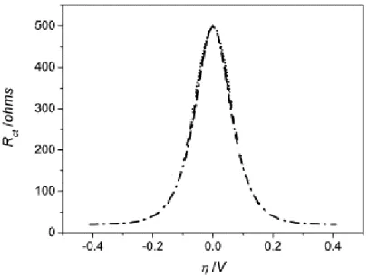
Fig. 4.6: Charge transfer resistance variation in function of the overpotential for a non rectifying system.

(Image adapted from [75])...37

Fig. 4.7: Equivalent circuit of the electrode/electrolyte interface considering the interfacial capacitance,

charge transfer resistance, diffusion resistance and spreading resistance. The electrode circuitry is to the left and the electrolyte is to the right...39

Fig. 4.8: Photography of the system used to stimulate the embryo. The glass constitutes the floor and the

PDMS cube constitutes the walls and roof of the channel. The inlets are the small holes visible at the chip surface. ...40

Fig. 4.9: CleWin design of the device (courtesy of S. Baranek). It corresponds to the system viewed from

above with the PDMS roof removed. The approximate channel dimensions are in Table 4.1. ...42

Fig. 4.10: Lateral (top) and frontal (bottom) views of the device. The block is about 5mm height. The

inlets are cylinders with 1.5mm diameter. The pillar is a cylinder with 20µm diameter. The approximate channel dimensions are in Table 4.1. Note: the draws are not scaled to the system dimensions...43

Fig. 4.11: Schematics of the setup used to measure the current and the bulk resistance of the channel. The

channel is represented by a box. The instrument for the measurement may be an ammeter or an

impedance spectrometer (both represented by an “A”)...45

Fig. 4.12: The approximate location of the new inlets (in blue) compared to the original inlets (in purple).

The blue section of the channel corresponds to the part where the electric current and fluid go, showing a decrease in both hydrodynamic and electric resistance. ...48

(14)

Fig. 4.14: Chip configuration using the agar salt bridges. The salt bridges are inserted in the inlets and

the electrodes are placed into the salt bridges instead of directly into the inlets. This avoids the contact between the electrodes and the electrolyte, while allowing an almost unchanged electric current. ...53

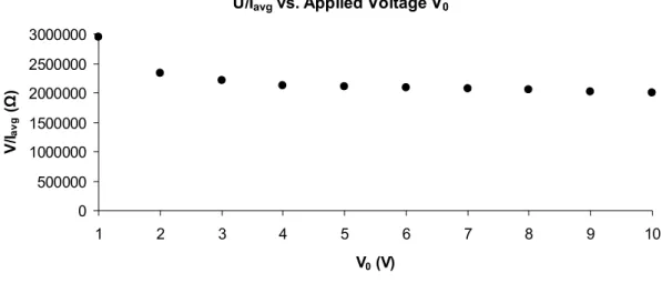
Fig. 4.15: Resistance obtained by applying Ohm’s law to the measured data, in function of V0 (two wire method)...55

Fig. 4.16: Voltage drop as a fraction of the initial voltage in function of the channel length for 2D

simulation, calculated by COMSOL. The x axis is in millimetre. The flattening of the curve at the

extremities is due to the electric field being almost constant at the inlets, and thus also the voltage. ...57

Fig. 4.17: Comparison between the voltage drop plot computed from the average values of the electric

field obtained from the measured current versus the plots of the voltage drop computed using the same method, but using the instead the average values obtained from the 2D and 3D simulations. The x axis goes from 0 to 6870µm...57

Fig. 4.18: Top: colour map of the current density profile at the embryo region. Bottom: colour map of the

electric field profile at the embryo region. The stream and field lines are visible. The scale is nA/µm2_for the current density and mV/µm for the electric field. Hot colours represent higher values and cold colours represent lower values. The size bar ranges from 0 till 4.76nA/µm2_{for the current density and 0 till} 2.19mV/µm for the electric field. The current goes from the left to the right. The coordinate axes are in 10-4_{m. Calculations performed by COMSOL. ...59}

Fig. 4.19: Relationship between the electric field and the temperature calculated at the embryo region by

COMSOL. ...60

Fig. 4.20: Schematic representation of the circuit analogy of the system. The central channel is

approximated by a resistor between the inlets, representing the bulk resistance Rbulk = 2.2MΩ. ...72

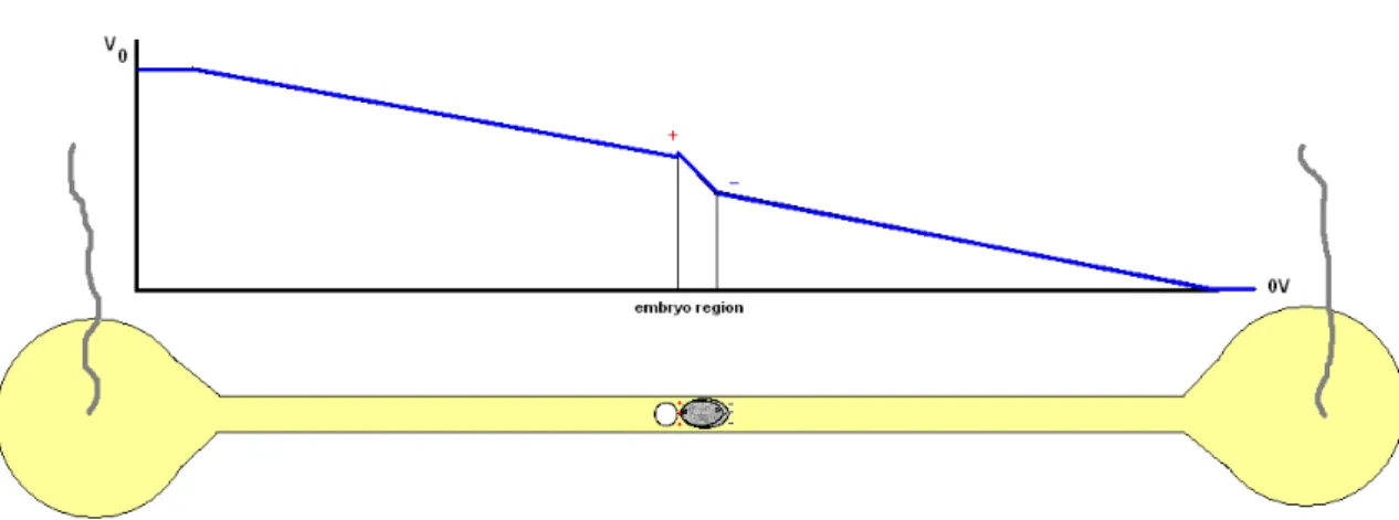
Fig. 4.21: Schematic representation of the voltage drop along the channel, evidencing the charge

accumulation around the embryo. ...73

Fig. 5.1: Schematic representation of the excess of accumulation of opposite charge at the anterior and

posterior extremities of the embryo (grey) that is placed next to the pillar (white). This excess of charge results from a greater charge gradient at the embryo extremities compared to any other part of the channel, and not from the presence of negative charge on one side and positive charge on the other side of the embryo...76

Fig. 6.1: Event timeline showing the selected events to analyse (see Table 6.2 and the list presented

previously). ...78

(15)

Fig. 6.3: DIC images of the 2-cell, 4-cell and 8-cell stages of the same embryo. (Image taken from [90])

...80

Fig. 6.4: First embryo cleavages and localization of the daughter cells. (Image adapted from [54]) ...81

Fig. 6.5: Mitosis of AB and P1 are accompanied by spindle rotation. This way the daughters remain oriented approximately parallel to the AP axis. (Image adapted from [91]) ...82

Fig. 6.6: Nomarski (DIC) time-lapse images of C. elegans gastrulation. Ea and Ep are pseudocoloured in green, and neighbouring cells are in blue. Arrows indicate the direction of the neighbouring cell movement. Top panel: lateral view with the P4 and MSxx labelled (MSx is in the first image and divides between the first and second images). Bottom panel: ventral view with Ea and Ep sinking into the embryo. Embryos are oriented anterior to the left. (Image and description taken from [92])...82

Fig. 6.7: Ventral (top) and lateral (bottom) views of the embryo at the lime-bean (left) and first comma

fold (right) stages. (Image adapted from [90, 93, 94])...83

Fig. 6.8: DIC time-lapse images of two embryos before hatching (left) and after hatching (right), where

the right juvenile worm is still leaving the egg. Although the images are unfocused, it is easily

distinguishable the empty eggshell left after hatching...83

Fig. 7.1: Injection procedure. 1) The embryo is mouth pipetted to a liquid drop on the top of one inlet of

the microfluidic chip already filled with PBS. 2) The drop with the embryo is sucked with the help of a syringe on the other inlet until the embryo is placed next to the pillar. 3) More liquid is injected in order to fill the inlets. 4) When the device is ready, the electrodes are inserted in the inlets and a voltage (V0) is applied between them. ...86

Fig. 7.2: Left: DIC image of the embryo in the correct position (psudocleavage stage). Right: Brightfield

image of the 2-cell stage embryo slightly oblique in the up-down direction, resulting in part of the P1 cell being under the AB cell. ...87

Fig. 7.3: Final setup of the system already placed at the microscope. In this experiment, salt bridges at

the inlets were used to avoid channel contamination with electrode products...87

Fig. 7.4: DIC image of two embryos at the 2-cell stage in a PBS drop on a coverslip...88

(16)

Fig. 8.1: Plot comparing the average of the control and electric field experiments temporal series. A

logarithmic scale was used. From the origin to the opposite extremity, the points correspond to the following time differences: tP0- tncl; tAB- tP0; tP1- tAB; tABa- tP1; tEMS- tABa; tP2- tEMS; tgstr- tP2; tfld- tgstr; tmov- tfld; tbrn- tmov. Control experiments are represented by the x axis and electric field experiments are represented by the y axis. ...96

Fig. 8.2: Average of the time differences of the eleven events that were statistically analysed. A

logarithmic scale was used. To compute the total average development time (since the firs cleavage), all the times must be summed. tP0- tncl was not considered for this computation. The number of experiments for each event is in Table 8.1...96

Fig. 8.3: Average of the time differences of the early events (until the division of P2) that were statistically analysed. The number of experiments for each event is in Table 8.1. ...97

Fig. 8.4: Average of the time differences of the later events (after division of P2) that were statistically analysed. The number of experiments for each event is in Table 8.1. ...97

Fig. 8.5: Cell cycles of the first three cells: Interphase, M-phase and entire cell cycle. For P0, only the Interphase after the pro-nuclei fusion was considered (*). The number of experiments for each event is in Table 8.4...99

Fig. 9.1: Diagram comparing the differences in division times between control and electric field

experiments, until the start of the 8-cell stage. The longer the line above the cell name, the longer is its cycle, except for P0, were the cell cycle duration is represented by the line below the cell name (since the diagram starts there). Note: the time is not precisely scaled by the line length. ...104

(17)

List of Tables

Table 4.1: Dimensions of the system channel ...42

Table 4.2: Relevant platinum electrode properties ...50

Table 4.3: Channel bulk resistance computed theoretically and measured experimentally ...54

Table 4.4: Average current density and average electric field computed from the average of the measured

current using the average channel dimensions ...55

Table 4.5: Comparison between the values of the current density and electric field computed from the

measurements versus the average values obtained from the 2D and 3D simulations (segments 3/3’ neglected) for V0 = 5V...56

Table 4.6: Comparison of the average current density and average electric field obtained from the 2D

simulation with no embryo and with embryo, both for V0 = 5V ...58

Table 4.7: Results of the computations of the parameters of the electrode/electrolyte interface...61

Table 6.1: Mean and standard deviation of duration (in minutes) of S and M phases in P0, P1 and AB determined by time-lapse DIC microscopy (20 embryos analysed) (Taken from [87])...79

Table 6.2: Time of events selected for analysis in relation to pro-nuclei fusion ...79

Table 6.3: Time of events selected for analysis in relation to the previous event ...79

Table 8.1: Number of observations of each of the eleven consecutive time differences statistically

analysed (Fig. 8.2 – 8.4)...94

Table 8.2: Temporal analysis results: Mean of the times of the events measured for control and electric

field experiments; Mann-Whitney p-value for each of the eleven consecutive time differences statistically analysed...94

(18)

Table 8.3: Standard deviation of the eleven time differences for control and electric field experiments (in

parenthesis is the value divided by the mean of the corresponding time event)...95

Table 8.4: Number of observations of the cell cycle times (Fig. 8.5)...98

Table 8.5: Mean of the times of the cell cycles of the first three cells of the embryo (P0, AB and P1) ...98

Table 8.6: Standard deviation of the cell cycles of the first three cells of the embryo (P0, AB and P1) (in parenthesis is the value divided by the mean of the corresponding time event)...99

(19)

Physical Quantities and Constants

Quantity Symbol Unit

Distance D, x Metre (m) Length L, l, d Metre (m) Width W, w Metre (m) Height h Metre (m) Radius r Metre (m) Diameter d Metre (m)

Area A Square metre (m2)

Electric Field E Newton per Coulomb

(N/C), Volt per metre (V/m)

Electric Current I Ampere (A)

Current Density J Ampere per square metre

(A/m2₎

Electric Potential V, E Volt (V)

Potential Difference or

Voltage U, V Volt (V)

Overpotential η Volt (V)

Thermal Voltage Vt Volt (V)

(20)

Resistivity ρ Ohm times square metre

(Ω.m2)

Conductance G Siemens (S), Siemens per

square metre (S/m2₎

Conductivity σ Siemens per square metre

(S/m2₎

Charge transfer Resistance RCT Ohm (Ω), Ohm times

square metre (Ω.m2₎

Diffusion Resistance Rd Ohm (Ω), Ohm times

square metre (Ω.m2₎

Spreading Resistance RS Ohm (Ω), Ohm times

metre (Ω.m)

Capacitance C Farad (F)

Interfacial Capacitance CI Farad (F), Farad per square

metre (F/m2₎

Helmholtz Capacitance CH Farad (F), Farad per square

metre (F/m2₎

Gouy-Chapman

Capacitance CGC Farad (F), Farad per square metre (F/m2)

Permittivity ε Farad per metre (F/m)

Vacuum Permittivity ε0 8.8542 Farad per metre

(F/m) Relative permittivity,

dielectric constant εr Dimensionless

(21)

Faraday Constant F 96485 Coulomb per mole

(C/mol)

Electron valence z Dimensionless

Temperature T Kelvin degree (K), Celsius

degree (ºC)

Gas constant R 8.3145 Joule per mole per

Kelvin (J/(mol.K))

Concentration of ion X [X] Mole per cubic metre

(mol/m3₎

(22)

(23)

Symbols and Abbreviations

2D: Two dimensional

3D: Three dimensional

AC: Alternating current

AP: Antero-posterior

BioMEMS: Biological Microelectromechanical systems

C. elegans: Caenorhabditis elegans

DC: Direct current

DIC: Differential interference contrast

DV: Dorso-ventral

E. coli: Escherichia coli

EEM: Extraembryonic matrix

EF: Electric field

FEM: Finite element method

NEBD: Nuclear envelope breakdown

PBS: Phosphate buffered saline

PDMS: Polydimethylsiloxane

(24)

(25)

Abstract

Bioelectricity has an impact on the development of tissues because it can influence cell polarization, essential for asymmetric cell division. This feature may be an important tool for tissue engineering and regenerative medicine applications.

The nematode Caenorhabditis elegans is a primitive organism, but whose physiology shares several characteristics of human biology. Its embryo is an ideal model for the study of cell division and embryogenesis, since its development is almost invariant and highly reproducible and readily observable.

This project has the objective of studying the impact of a DC electric field in the

C. elegans embryo development and to assert if this organism is a good model for

further research in this field. To accomplish it, a DC electric field is applied in a microchannel filled with PBS, where to the embryo is confined.

Embryogenesis is studied by analysing selected development stages, which are compared for control and electric field experiments. To optimize the application of the electric field to the embryo and minimize other physical phenomena which can disturb embryogenesis, a detailed physical characterization of the microfluidic system is also performed.

The results show that there are no big differences in the events of embryogenesis, suggesting that the embryo resists to the electrode field, perhaps due its eggshell. Nevertheless, small differences in embryological times suggest that the electric field can have long term effects on embryogenesis, and that a more detailed analysis should be performed.

In summary, the embryo nematode C. elegans is not as suited to study the impact of DC electric fields in embryogenesis as other embryo models, such as amphibians. However, there is still the possibility of studies of single isolated embryo cells. Besides, it is not discarded the possibility of applying an AC electric field or attempting to remove the eggshell in future studies.

Keywords: C. elegans embryogenesis; Asymmetric cell division; Bioelectricity; DC

(26)

(27)

Resumo

A bioelectricidade pode influenciar a polarização de uma célula, responsável pela divisão assimétrica, pelo que tem um impacto significativo no desenvolvimento de tecidos ao contribuir para controlar a migração e orientação de células e também a proliferação, diferenciação e apoptose celulares. Estas propriedades da bioelectricidade em tecidos biológicos tornam-na numa ferramenta importante em engenharia de tecidos e medicina regenerativa, pois permite controlar várias respostas fisiológicas a estímulos eléctricos e usá-las para fins benéficos.

O nematóide Caenorhabditis elegans é um organismo primitivo, mas cuja fisiologia partilha várias características da biologia humana. Estas características, juntamente com a sua simplicidade de cultivar em grandes populações e de ser conveniente para análise e manipulação genética, tornam-no num dos organismos-modelo mais vastamente utilizados em investigação científica, existindo actualmente uma enorme quantidade de informação disponível sobre este nematóide. O embrião do

C. elegans representa um modelo ideal para o estudo da divisão celular e da

embriogénese, visto que o seu desenvolvimento é altamente reprodutível e facilmente observável. Além disso, o padrão de desenvolvimento do embrião é praticamente invariável, tornando possível construir um diagrama que representa toda a sua linhagem celular, o que facilita imensamente a análise da embriogénese.

A motivação deste projecto surge do conhecimento de que vários seres vivos, como a hidra ou a salamandra, possuem uma grande capacidade de regeneração que está grandemente relacionada com a bioelectricidade. Compreender e controlar os seus mecanismos será certamente um grande avanço na área de engenharia de tecidos e terá como consequência o surgimento de diversas potenciais aplicações.

Este projecto tem como objectivo aplicar a aplicação de um campo eléctrico DC num organismo vivo, de forma a induzir uma resposta por parte dele. Devido às suas características, o embrião do nematóide C. elegans foi escolhido como organismo modelo para a aplicação deste estímulo eléctrico. A principal assumpção é que o campo eléctrico aplicado ao longo do eixo antero-posterior do embrião do nematóide C.

elegans, induza uma acumulação de carga oposta nas suas extremidades anterior e

(28)

de poderem induzir respostas celulares diferentes em cada extremidade, causando alterações na embriogénese. A ideia surge de uma analogia à aplicação de um gradiente de temperatura ao longo desse mesmo eixo, sabendo-se actualmente que induz uma resposta relativamente à duração de ciclos celulares, visto que é fortemente dependente da temperatura.

Através dos resultados, pretende-se também avaliar a utilidade deste embrião como um organismo-modelo para o estudo do impacto de campos eléctricos DC em tecido vivo, visto que outros embriões, como de anfíbios ou pintos, apresentam grandes distúrbios no seu desenvolvimento quando estimulados com campos eléctricos contínuos, com consequências catastróficas no organismo final.

A tecnologia dos micro-sistemas permite controlar eficazmente o ambiente celular de uma forma bastante precisa. Assim, um sistema microfluídico é usado como plataforma para estudar o impacto da aplicação do campo eléctrico ao embrião. Este é colocado no interior de um microcanal contendo PBS (tampão fosfato-salino), um bom electrólito e ao mesmo tempo biocompatível para o seu desenvolvimento. Recorrendo a eléctrodos de platina, é aplicada uma diferença de potencial nas extremidades do canal, o que torna possível a existência de uma corrente eléctrica que deverá resultar numa acumulação de carga oposta nas extremidades do embrião, visto que a sua resistividade deverá ser superior à do PBS. A largura e altura do canal são semelhantes à espessura do embrião, o que garante que o campo eléctrico passa através do embrião ou que seja desviado por ele, no caso de este ser isolante.

Tendo em conta que o campo eléctrico propaga-se através do canal em direcção ao embrião, é necessário saber qual a sua magnitude à volta dele. Além disso, interacções físicas como o efeito de Joule e reacções redox entre os eléctrodos e o electrólito podem alterar a temperatura e o pH no interior do canal e comprometer o desenvolvimento do embrião de forma indesejada. Assim é também efectuada uma caracterização física detalhada do sistema microfluídico, com o intuíto de saber quais os principais fenómenos físicos que podem ocorrer no interior do canal durante a aplicação do campo eléctrico. Esta caracterização permite tomar as medidas necessárias para minimizar estes efeitos secundários que possam perturbar o normal desenvolvimento do embrião.

(29)

constituinte do PBS e em determinar a relação entre a corrente eléctrica no canal e a diferença de potencial aplicada. Para isso são efectuadas medições experimentais e simulações recorrendo ao software de elementos finitos COMSOL Multiphysics.

O procedimento experimental para a análise do impacto do campo eléctrico no embrião começa com a recolha de um embrião de um nematóide hermafrodita adulto, proveniente de uma cultura em pratos de agarose semeados com Escherichia coli como fonte de alimento. O embrião escolhido deve estar no início do desenvolvimento, de preferência após a meiose, de forma a poder ser estimulado o mais cedo possível. Sabe-se que perturbar os eventos iniciais da embriogéneSabe-se pode ter conSabe-sequências em todo o restante desenvolvimento, visto que este depende grandemente das primeiras divisões celulares.

Recolhido o embrião, este é inserido no microcanal, onde é fixado e permanece durante todo o ensaio experimental. De seguida, o campo eléctrico é aplicado através da aplicação de uma diferença de potencial nos eléctrodos em contacto com as extremidades do canal. Pontes salinas de agarose são utilizadas em algumas experiencias para evitar a contaminação do electrólito com produtos das reacções químicas que ocorrem na superfície dos eléctrodos. O desenvolvimento do embrião é observado através de microscópios invertidos equipados com contraste de fase. Imagens de time-lapse são capturadas e posteriormente analisadas recorrendo ao software

ImageJ. Eventos da embriogénese seleccionados para análise são comparados para

embriões em experiencias de controlo e embriões estimulados com o campo eléctrico. Métodos de análise estatística são efectuados para auxiliar a comparação. Parâmetros a observar e comparar são os tempos de ocorrência dos eventos seleccionados e orientação e posição de células no embrião. O comportamento da minhoca juvenil após o nascimento também pode fornecer informação relativamente à embriogénese, pelo que também é analisado.

A caracterização do chip revelou que uma tensão de 5V é apropriada para criar um campo eléctrico com dimensões fisiológicas (cerca de 0.3mV/µm), não aumentando a temperatura para valores fora dos limites de desenvolvimento normal do embrião. Alterações do pH foram minimizadas através da utilização das pontes salinas inseridas nas entradas do canal.

A comparação entre embriões de controlo e embriões estimulados revela que não existem grandes diferenças entre os eventos da embriogénese de embriões de controlo e

(30)

embriões estimulados pelo campo eléctrico, o que sugere que o embrião resiste ao campo eléctrico, talvez devido à barreira de permeabilidade presente na sua carapaça. Pequenas diferenças nos tempos embriológicos entre embriões de controlo e estimulados sugerem que o campo eléctrico possa ter efeitos a longo prazo na embriogénese, retardando os seus eventos mais tardios. As diferenças são demasiado pequenas para se poder tirar alguma conclusão, contudo, os resultados sugerem que deveria ser feita uma análise mais detalhada ao ciclo celular de certas células do início da embriogénese, o que não foi possível com o equipamento disponível.

Comparando estes resultados com os de outros estudos com embriões, como por exemplo em anfíbios ou pintos, conclui-se que o impacto do um campo eléctrico DC no desenvolvimento do embrião do nematóide C. elegans não é tão significativo como nesses modelos, o que os torna preferíveis para estudos com embriões intactos. No entanto, existe ainda a possibilidade de estudos a nível de células isoladas extraídas do embrião e também não é de descartar a hipótese de aplicar um campo eléctrico AC ou de tentar remover a carapaça do embrião em futuras investigações.

Palavras chave: Embriogenese do C. elegans; Divisão assimétrica; Bioelectricidade;

(31)

Acknowledgements

First of all, I have to thank my parents and siblings for all the help, support and motivation they gave me during the roughest times when I was writing this thesis. I am really grateful to Professor Philippe Renaud who gave me a unique opportunity and continuously provided helpful suggestions when my project faced an apparent dead end.

I am also grateful to Professor Abel Oliva, without him I would never had this opportunity.

I sincerely thank my supervisor at EPFL, Robert Meissner, from whom I a have learnt a lot during this year. I am grateful for his constant availability and for all the times he explained or taught me about something I didn’t know or wasn’t familiar with. Without him, I would be permanently lost in the lab.

I would like to thank Hugo Ferreira, for his almost instantaneous suggestions to solve a particular problem and for all the help and patience while I was writing the report. I have to thank Sophie Baranek for teaching me about C. elegans, Harald van Lintel and Arnaud Bertsch for the help with every type of devices and their sense of humour, and the remaining crew of LMIS4. I also thank Pierre Gönczy, Coralie Busso, Aitana Neves, Alexandra Bezler and Simon Blanchoud from the SV lab, who were always available to help me with C. elegans.

I thank Wyllian Hasenkamp and Daniel Duplat, the two whom I could speak portuguese in the middle of that sea of foreigner languages.

I would also like to thank the professors of IBEB, Alexandre Andrade and Eduardo Ducla Soares, and also to Giomar Evans.

Finally, I thank the friends I have made in Lausanne, namely Mafalda, Ricardo, Aleksey and Arthur, with whom I shared the final moments during my stay in Switzerland.

(32)

(33)

1. Electricity of Life

1.1. What is Bioelectricity?

Electricity is everywhere in our lives. Everything we see, hear, fell, touch or think is electricity. Our sense of reality is in fact the interpretation of electric signals by the brain, making our perception of life how it is. But electricity is not only in our senses. It is everywhere in our body. Our heart beats because of electricity. We move and speak because of electricity. We grow and reproduce because of electricity. If electricity did not exist, life would not exist. Electricity is present in every single cell that makes part of us and all other living beings.

Bioelectricity is the electricity produced by or occurring in living cells, tissues and organisms. The first evidence of how electricity can affect living organism goes back to the XVIII century, when the french clergyman Jean-Antoine Nollet caused 180 of the King’s guards to leap simultaneously by having them all hold hands and then connecting the man at the end of the line to the discharge from a Leyden jar [1]. The italian anatomist and physician Luigi Galvani was one of the pioneers to investigate experimentally the phenomenon that came to be named “bioelectrogenesis”, the ability of a living organism to generate electricity. In 1794, he proved that animals could generate electricity when he demonstrated that the cut end of a frog sciatic nerve from one leg induced contractions when it touched the muscles of the opposite leg (Fig. 1.1), introducing the concept of “animal electricity” [2]. Galvani's famous experiments helped to establish the basis for the biological study of neurophysiology and neurology [2].

In 1843, the swiss-german scientist Emil Heinrich Du Bois-Reymond measured a small current flowing out of a cut in his own finger [1] and five years later he used a galvanometer (named after Galvani) to detect what he called an “action current” in the frog's nerve, later called by “action potential”. Reymond’s work created the field of scientific electrophysiology as the science that studies bioelectricity, which greatly

(34)

contributed to reduce physiology to applied physics and chemistry, a trend that has dominated physiology and medicine ever since [2].

In modern times, the measurement of bioelectric potentials has become a routine practice in clinical medicine. Electrical effects originating in active cells of the heart and the brain, for example, are commonly monitored and analyzed for diagnostic purposes.

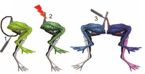
Fig. 1.1: Galvani’s experiments using a frog leg preparation. The leg contracted when the cut end of the

sciatic nerve touched the leg muscle (1) or when the electrical discharge was applied directly to the nerve (2). When the surface of a section of the right sciatic nerve touched the intact surface of the left sciatic nerve, both legs contracted (3). (Image taken from [1])

Currently, bioelectricity is defined as electric potentials and currents produced by or occurring within living organisms. Bioelectric potentials are identical to the potentials produced by devices such as batteries or generators, but are instead generated by a variety of biological processes and are also weaker, generally ranging in strength from only one to a few hundred millivolts [3]. The most famous bioelectric potential is the action potential, used to transfer information in animals and playing a central role in cell-cell communication. Bioelectric currents, on the other hand, are always ionic, differing completely from the electron currents flowing in metal wires. In animals, bioelectric currents occur due to the movement of ions through the interstice, cytoplasm and across cell membranes, through ion channels. Their strengths usually range from hundreds of nanoamperes to hundreds of microamperes.

(35)

The potential across the cell membrane i.e. the difference between the potential inside the cell and the potential outside the cell is called the membrane potential (Vm). No

single ion species is distributed equally on the two sides of a cell membrane. There are four most abundant ions found on either side of it: Na+ and Cl- are more abundant outside the cell and K+ and organic negative anions are more concentrated inside. The cell is impermeable to organic ions due to their size, but not to the other three ions, which are allowed to move across the membrane through ion channels. The membrane potential that results from the total contribution of those three ions is given by the Goldman equation [4]:

 

i Na

 

i Cl

 

o K i Cl o Na o K m Cl P Na P K P Cl P Na P K P zF RT V _ _ _         ln (1.1)

PX is the permeability of the membrane to the ion X. This permeability results from the

activity of specific ion channels and may be influenced by voltage gradients, chemical gradients and mechanical stress. Therefore, the activity of these channels may change due to internal stimulus induced by the cell or external stimulus induced near it.

At a specific potential, the currents from all the ions cancel each other and the total current at the membrane is zero (IK + INa + ICl = 0). In this situation, the membrane is said

to be at rest, and its potential is called the resting membrane potential (Vr). Almost all

cell membranes are polarized at rest, since Vr is never equal to zero. However, the

activity of a cell may change when its polarization (i.e. its membrane potential) changes from the rest situation, due to a stimulus.

Cell membranes also show a capacitive effect. This is extremely important, because the membrane is very thin and thus highly capacitive [5]. A capacitive or displacement current is responsible for charging the membrane when electrical stimuli are applied to it, and thus changing the membrane potential. It is crucial for the propagation of the action potential, for example.

(36)

dt dV C I m m C  (1.2)

Cm is the membrane capacitance. At rest, the capacitive current (IC) is zero since Vm does

not change with time.

Ionic currents do not exist only at the cell membrane. They exist also inside the cell, in the cytoplasm, and outside the cell, in the interstice, and may cross the cell membrane, creating electric circuits. Ionic currents may also flow away from a cell and cross entire tissues, due to electric fields gradients induced by the membrane potential of various cells. These electric fields are responsible for many regenerative and growth processes.

1.2. Asymmetric Cell Division and Tissue Growth and

Development

Bioelectricity has a great impact in tissue development and growth, because it can influence cell polarization. Cell polarity does not refer to membrane charge gradients, but instead to spatial differences in the shape, structure, and function of cells. A complete organism is not symmetric. Mammals have a head at their rostral extremity and two feet at their ventral extremity. The human heart is on the left side and not on the right. How can this happen if all animals started as a unique round egg cell? Also, how can a vertebrate have a nervous system and a skeleton, two completely different tissues, if both of them came from the same cell? The answer is asymmetric cell division.

Asymmetric cell division is the process that allows one cell, called stem cell, to divide into two daughter cells with different fates (Fig. 1.3). These divisions allow cellular diversity, an essential feature of the development of any multicellular organism [6]. Through asymmetric divisions, stem cells can both generate differentiating cells that will constitute the bulk of the tissues, and self renew, thereby maintaining a constant

(37)

pool of stem cells (Fig. 1.2). Two distinct mechanisms (or a combination of them) can lead to asymmetric cell divisions [6]:

 Extrinsic mechanisms: two daughter cells are born equal but an asymmetry is subsequently induced in one of the daughters by the cell environment or cell niche;

 Intrinsic mechanisms: two daughter cells are born different after determinants are segregated asymmetrically before division. The three main events required for such process to occur are polarization of the mother cell, unequal distribution of cell fate determinants along the polarity axis and proper alignment of the mitotic spindle in the axis of polarity. Cell polarity is the trigger for the other two events that occur after. It arises primarily through the localization of specific proteins to specific areas of the cell membrane.

Protein localization requires both the recruitment of cytoplasmatic proteins to the cell membrane and polarized vesicle transport along cytoskeletal filaments to deliver transmembrane proteins from the Golgi apparatus. Examples include the PAR complex (Cdc42, PAR3, PAR6, atypical protein kinase C), Crumbs complex (Crb, PALS, PATJ, Lin7), and Scribble complex (Scrib, Dlg, Lgl) [7]. Most of them are common among several different organisms.

Fig. 1.2: A stem cell divides asymmetrically originating two daughter cells with different fates. The

daughters may differentiate and proliferate or remain stem cells to divide asymmetrically again. A healthy tissue is composed by several differentiated cells. (Image taken from [6])

After an asymmetric division, the two daughter cells may have completely different fates. They can differentiate and proliferate to form various tissues or remain

(38)

undifferentiated. They can migrate to different places and orient to different directions. They may even be destined to die by apoptosis.

Fig. 1.3: Asymmetric division of the egg-cell of three different organisms. This is the first mitotic

division of embryogenesis. The polarized mother cell during anaphase is shown at the top of each panel, whereas the daughter cells that are produced by asymmetric division are shown at the bottom of each panel and are named below. The distribution of several components that are important for polarity establishment, spindle positioning and cell-fate determination is illustrated for the mother cell, and the distribution of cell-fate determinants is shown for daughter cells immediately after mitosis. Note that many of them are the same for the three organisms. Directional signalling between the anterior cell (pIIb) and the posterior cell (pIIa), whereby the Delta ligand from pIIb signals to the Notch receptor on pIIa, is denoted by a thick arrow in panel c. This is an example of an extrinsic mechanism of fate determination. (Image and description taken from [8])

1.3. The Impact of Bioelectricity in Regeneration and

Development

By affecting cell polarization, bioelectricity contributes to control cell fate, as the cell orientation, directionality of cellular migration and differentiation. DC electric signals

(39)

inflammation responses. This level of physiological control allows coordinating complex regenerative responses, as the wound healing in humans or limb regeneration in salamanders.

The transepithelial potential (TEP) is the potential difference across an intact epithelium and arises from its impermeability due to tight junctions between cells that block the flow of ionic currents. After an injury, the epithelium is interrupted creating a current leak at the wound site causing an immediate collapse of the TEP at the wound. This injury current creates a steady voltage drop that decreases within the distance to the wound, which, by its turn, creates an extracellular DC voltage gradient, strongest at the wound region and weaker as the distance to the wound increases (Fig. 1.4). Injury currents were first observed during Galvani’s experiments with the frog nerve, but also may occur at other tissues that have a TEP, such as the skin, as showed by Du-Bois Reymond [1].

The wound induced endogenous DC electric field may be present for hours, days, or even weeks during both development and regeneration [1]. The regeneration mechanism eventually involves adult stem cell divisions and differentiation in order to recreate the missing tissue. The electric fields are though to be involved mainly in the cell orientation and migration mechanisms, a phenomenon termed electrotaxis. It consists in the movement of charged receptor molecules, exposed on the outer surface of the cell membrane lipid bilayer, due to the physical action of a physiological electric field. This results in a created receptor asymmetry between cathodal and anodal facing membranes, that in turn induce asymmetries in the cellular response (by signal transduction), that may affect the cell division [9].

As an example is the division of human corneal epithelial cells, whose cleavage plane orients perpendicularly to an artificially applied DC electric field [10] (Fig. 1.5). It was also shown that they tend to migrate in direction to the cathode, when submitted to an electric field [11]. Other studies showed that wounded rat corneal epithelium regenerated differently when the endogenous injury electric field was manipulated. The rate and degree of wound healing was proportional to the magnitude of the electric field that was increased or decreased by changing the transcorneal potential difference through chemical treatments that altered the epithelium permeability to ions, such as

(40)

Na+ and Cl-, that are needed to create injury currents [12, 13, 14]. These results showed that disrupting the injury currents alters tissue regeneration.

Fig. 1.4: Top: skin epithelium of the Xenopus embryo. The transepithelial potential results from active

transport and passive diffusion of ions across the basal and apical membranes of epithelial cells. Thigh junctions avoid the passage of ions outside the cells. Bottom left: wounding of an epithelial sheet (or localized disruption of tight junctions) creates a current leak at the wound site causing the immediate, catastrophic collapse of the TEP at the wound. The TEP is not affected distally, where the epithelial integrity and ion transport properties remain intact. Na+leak out the wound, resulting in an outward injury current and a lateral voltage gradient (electric field) within the embryo (green arrows) oriented parallel to the epithelial sheet. The wound site is the cathode of the EF. Bottom right: circuit model of the wounded epithelium. Each battery represents the transepithelial potential for a patch of epithelium. It differs with the distance to the wound. Rw is the resistance of the wound, Rfluid is the resistance of the pound water where the frog embryo develops and Rtissue is the resistance of the tissue underlying the epithelium. (Image taken from [1])

Experiments using neuron cultures submitted to DC electric fields demonstrated that the nerve growth was enhanced and directed by the field, showing that electrotaxis is involved in neural tissue growth [9]. Measurements in intact amphibian embryos show spatial differences in the TEP that generate electric fields within them. Altering those fields by electrical stimulation disrupts embryogenesis [15]. Large currents flowing out the cut end of a newt amputated limb were also detected and persisted during all the regeneration process. Interestingly, the currents stopped when skin grafts covered the wound region, suggesting that the regeneration ends when the skin is covering again the wound [16]. Other examples of research about the impact of bioelectricity in tissue

(41)

Fig. 1.5: Orientation of the cleavage plane of transformed human corneal epithelial cells was affected by

applied EFs (strength and polarity as shown). (a) No field control. Cleavage furrows are evident and oriented randomly. (b) Dividing cells in an applied EF showed preferential orientation of the cleavage furrow. (Image and description taken from [10])

The response of stem cells to DC electric fields shows bioelectricity as a very important tool in tissue engineering and regeneration medicine. The potential applications of manipulating biologic tissue with these fields are apparent. Once understood their mechanisms, one can use the interaction between bioelectricity and a tissue for beneficial ends. Chronically wounds could be healed and born body deficiencies could be minimized or completely eliminated. The most prominent potential applications nowadays are in cancer research and spinal cord regeneration.

Cancer cells have a greater negative surface charge than normal cells, and usually their membrane potential is depolarized markedly. The TEP of the skin of normal and cancer breast epithelium differs, and this is used clinically to diagnose the early onset of breast cancer in women [1, 19, 20]. There are also reports of small steady extracellular voltage gradients between cancerous tissue and neighbouring normal tissue, which could act as guidance cues promoting and directing cancer cell migration [1, 21]. In rat prostate cancer tissue, cell lines with different metastatic levels responded differently to an external applied electric field, suggesting news therapies to this disease [22].

(42)

Borgens [23, 24, 25] was able to restore some function in damaged guinea pig spinal cord with an applied DC electric field. The electric field stimulated and directed regenerative growth of large numbers of myelinated axons towards the cathode. The degree of regeneration was enough to allow certain specific reflexes to occur. Who knows if in the near the future there will exist implantable stimulating devices for entire spinal cord regeneration, or to electrically kill cancer cells and destroy tumours.

(43)

2. Motivation and Objective

When observed in other animals such as the salamander or the starfish, everybody certainly has thought at least once why limb regeneration does not happen in humans. They eventually have also wondered if in a far future technology would not be advanced enough to allow this phenomenon to occur on us. The latest advances in science are showing, however, that the so called “future technology” is not an illusion, but a possibility that may turn into reality very soon. In medicine and also in other sciences, several techniques that seemed impossible ten years ago are routine nowadays. Who knows if limb regeneration, chronic wound healing, spinal cord repair or cancer elimination will not be a reality in the next years?

This project is based on the context of tissue engineering and is concerned in understanding how bioelectricity and living tissue interact. To achieve this goal, the embryo of the nematode Caenorhabditis elegans will be used as model to study the impact of a DC electric field in tissue development. The embryo seems to be ideal for this particular study, since its embryogenesis is highly reproducible, allowing to easily observe asymmetric division and cell migration and orientation.

Furthermore, a previous study [26] showed that this particular embryo responds to a gradient of temperature applied across its antero-posterior (AP) axis, which induces a change in its development pattern. In a similar way, an electric field gradient across the embryo might induce a change in embryogenesis, due to the electrically induced polarizations in the embryo cells.

The objective of this project is to apply a DC electric field to the embryo of C. elegans and analyse whether responses in it occur or not. The hypothesis assumed here is that, applying a DC the electric field across the AP axis of the embryo, an excess of negative charge will accumulate on one side of the embryo and an excess of positive charge will accumulate on the other side, resulting in a different cell membrane polarity at different parts of the embryo. In an analogous way to electrotaxis, it is expected that possible cellular responses resulting in abnormal cell polarizations will change asymmetric division mechanisms and alter the development of the embryo.

(44)

In order to successfully apply the electric field to the embryo, a microchannel filled with conductive and biocompatible medium will be used. Due to its small and rectangular dimensions, the field can be easily directed and focused to the AP direction of the embryo. Some physical processes occurring in the channel may disturb the embryo development, so a detailed characterization of the physics at the channel will also be performed. To accomplish that, experimental measurements, simulations and a theoretical analysis will be used to model the microfluidic system.

The characterized system will then be used to conduct experiments where the C. elegans embryo will be stimulated with a DC electric field, and any differences between normal and stimulated embryogenesis will be analysed. The experiments will be conducted under certain assumptions that depend on the system characterization and must be in accordance wit the goal of the project.

In order to correctly analyse the C. elegans embryo development, some details of its embryogenesis must also be asserted a priori and used as a template in which the study of the embryo will be based on.

(45)

3. Caenorhabditis elegans – Closer than it Looks

Biological models are widely used in research to study biological processes in a controlled manner. In tissue engineering, they range from individual cells, useful to study cell cycle and division, proliferation and differentiation, to entire organisms, namely embryos in-vitro to study embryogenesis and development and amphibians to study tissue growth and regeneration. Some invertebrates and microorganisms are also widely used, since they are simpler and usually have great capacities of regeneration. Tissues in culture, on the other hand, allow studying developmental processes under simple and controllable biological conditions [27].

One of the most appropriate models to study cellular and development mechanisms is the nematode Caenorhabditis elegans. It is a primitive organism that shares several biological characteristics that are central problems of modern human biology. It was initially chosen as a model by Brenner in 1996 [28] due to its simplicity to culture in great numbers and being convenient for genetic analysis and manipulation. At the present, it is one of the models most used in research. It was also the first organism whose genome was entirely mapped [29].

3.1. C. elegans Biology

Caenorhabditis elegans is a small (about 1mm long), free-living soil nematode

(roundworm) that lives in many parts of the world by feeding on microbes, primarily bacteria. The organism arises from only one cell, the egg, which suffers a complex development process, starting in an embryonic cleavage followed by morphogenesis and finally a growth till the adult stage. It produces sperms and oocites, mates and reproduces. After reproducing, it gradually ages, loses vitality and dies about 2/3 weeks after being born (Fig. 3.2). The development and function of this diploid organism are coded by around 20 000 genes [30, 31].

(46)

In the adult stage there are two genres, one hermaphrodite composed by 959 somatic cells and a male composed by 1031 somatic cells. Males are extremely rare, being only 0.05% of the total population. Despite this, sexual reproduction is preferred compared to asexual every time a male is available. The adult essentially consists in a tube which contains two smaller tubes. The outer tube (body wall) consists in the cuticle, hypodermis, excretory system, neurons and muscles, and the inner tube consists in the pharynx, intestine and, in the adult, gonads (Fig. 3.1). All these tissues are under an internal hydrostatic pressure, regulated by an osmoregulatory system [32]. Most of the animal volume consists in the reproducing system (gonads), formed by two individual tubes in the first and two thirds of the worm.

Fig. 3.1: Anatomy of an adult hermaphrodite C. elegans individual. A: DIC image of an adult

hermaphrodite. B: schematic drawing of its anatomical structures. (Image taken from [32])

After hatching, the animal goes through four juvenile stages (L1 – L4) (Fig. 3.3), then enters to the adult stage, highlighted by the beginning of the reproduction. In starving or overpopulation conditions, the worm at the L2 stage, instead of passing to L3, metamorphoses to an alternative stage called the Dauer state (L2d) [33]. Here, the juvenile nematode delays its development to adapt itself to the extremely adverse environments. It does not age or reproduce and can stay in the Dauer stage for more than 3 months, about four times its normal life span. After exiting the Dauer state, the

(47)

Fig. 3.2: Life cycle of C. elegans at 22ºC. The time of fertilization is set to 0. Numbers in blue along the

arrows indicate the length of time the animal spends at a certain stage. The first cleavage occurs at about 40min after fertilization. Eggs are laid outside at about 150min after fertilization, during the gastrulation stage. The length of the animal at each pos-embryonic stage is marked next to the stage name in micrometers. C. elegans embryogenesis will be presented in the next section. (Image and description taken from [32])

Despite its simple anatomy, the C. elegans displays many different behaviours including locomotion, foraging, feeding, defecation, egg laying, metamorphosis, sensory responses to touch, smell, taste and temperature as well as some complex behaviours like male mating, social behaviour, learning and memory and dependence [34, 35]. More detailed descriptions of the C. elegans biology can be found in [29, 32, 36, 37, 38, 39] and various other literature easily available through a simple search for the term “c elegans”.

(48)

Fig. 3.3: DIC images of the larval stages of C. elegans. (Image taken from [32])

3.2. C. elegans as a Model

There are a lot of reasons to use C. elegans as a model organism. As already stated, it is a primitive organism, thus simple to analyse, and possesses a lot of biological characteristics present in human beings. Among them are embryogenesis, morphogenesis, organogenesis, growth, aging, nervous function, behaviour, all of them determined by genes that can be manipulated [30]. In addition, its short life span makes it very useful for research about aging. All 959 somatic cells are transparent and visible with an optical microscope equipped with differential interference contrast (DIC)1, which allows examining the nematode till the cellular level in living preparations,

1_{DIC (Differential interference contrast microscopy or Nomarski microscopy) is an optical microscopy}

technique used to enhance the contrast in unstained, transparent samples, which contain little or no optical contrast when viewed using brightfield illumination. DIC is widely used to visualize cellular features, most notably nuclei and nucleoli, but also microtubules, chromosomes and cytokinesis furrows. Cells above or below the DIC focal plane are not visible, making this technique perfect to observe and follow