Diogo Alexandre Marques Soares
Optimisation of algorithms to predict biomass and
size distribution of fish reared in cages, using the
Aquanetix production management software
Universidade do Algarve
Master in Aquaculture and Fisheries
3
Diogo Alexandre Marques Soares
Optimisation of algorithms to predict biomass and
size distribution of fish reared in cages, using the
Aquanetix production management software
Master in Aquaculture and Fisheries
Specialization Aquaculture
Thesis supervision by: Internal coordinator: Professora Doutora Elsa Alexandra Martins e Silva Cabrita, Professora Auxiliar da Universidade do Algarve External coordinator: Doutor Diogo Fernandes Thomaz, Aquanetix, Reino Unido
Universidade do Algarve
2018
5
Optimisation of algorithms to predict biomass and
size distribution of fish reared in cages, using the
Aquanetix production management software
Declaração de autoria de trabalho:
Declaro ser o(a) autor(a) deste trabalho, que é original e inédito. Autores e trabalhos consultados estão devidamente citados no texto e constam da listagem de referências incluída.
6 A Universidade do Algarve reserva para si o direito, em conformidade com o disposto no Código do Direito de Autor e dos Direitos Conexos, de arquivar, reproduzir e publicar a obra, independentemente do meio utilizado, bem como de a divulgar através de repositórios científicos e de admitir a sua cópia e distribuição para fins meramente educacionais ou de investigação e não comerciais, conquanto seja dado o devido crédito ao autor e editor respetivos.
I
Acknowledgements
À Professora Doutora Elsa Alexandra Martins e Silva Cabrita por ter aceite ser minha orientadora interna e por todo o acompanhamento nesta etapa.
Ao Doutor Diogo Fernandes Thomaz, por me ter proporcionado esta experiência, por ter aceite ser meu orientador externo, por toda a ajuda prestada durante todo o processo de execução e elaboração da tese, pela disponibilidade e apoio, ensinamento e compreensão ao longo de todo o trabalho e pelas diversas chamadas no Skype. Foi sem duvida incansável a ajuda prestada.
Ao Doutor Mateo Ballester Moltó, por toda a ajuda, paciência e ensinamento na parte zootécnica do trabalho.
A toda a equipa da Piscialba, por me terem incluído na empresa, por toda a ajuda que me deram enquanto lá estive e por todos os bons momentos que me proporcionaram. Aos meus pais, por mais uma vez terem acreditado nas minhas capacidades e por me terem permitido concluir mais uma etapa da minha vida. Por terem estado comigo, embora longe, quando mais precisei deles.
Ao meu irmão, que apesar de mais novo, providenciou o maior apoio, pelo incentivo, motivação que me deu nesta fase e principalmente pela paciência.
A todos os meus amigos, por darem aquela força extra. Especialmente à Catarina, por ter ouvido todos os meus desabafos, pela paciência, pelo apoio que me deu e por toda a amizade.
Aos The Pretty Reckless cujas músicas me acompanharam ao longo desta etapa.
O meu muito obrigado!! Diogo Soares, Setembro 2018
III
Abstract
This Thesis aims to optimise the algorithms used to estimate actual biomass and weight distribution in gilthead sea bream (Sparus aurata) and European sea bass (Dicentrarchus labrax) cages by the Aquanetix Software. For this, we first try to understand the practical functioning of a fish farm that uses cages and how can the used procedures affect the collection of data or its veracity. Then, we use the data collected by the company and the observations made on the field in order to attempt the optimization of the algorithms that estimate biomass and weight distribution of the Aquanetix Software. The data parameters analysed were the moving average of the estimated biomass, mortality, density, number of fish and mean weight. Two time periods were tested for the moving average of the estimated biomass, at fourteen and thirty days prior to the first harvest. Between these two periods, the one at thirty days seemed to provide the better biomass estimation. Mortality and density showed to have no apparent influence in the deviations found between the biomass estimations and the total biomass harvested. The number of fish was found to be overestimated in the majority of the studied cages (n=7), with the exception of only cage 109. The mean weight was found to be underestimated in the majority of the studied cages, with the exception of only cage 03.
At the end, all proposed goals were achieved. In conclusion, every cage of sea bream studied (n=4) shows an under estimation of the mean weight of fish at first harvest, which in turn leads to an underestimation of the biomass. This suggests that every sea bream cage is currently being under fed, most likely, due to a fault on the feeding model which is probably overestimating the specific feeding rate (SFR) for this species. Alterations should be made to the feeding model in order to resolve this unbalance. The results for the sea bass cages were shown to be more inconclusive since all of the studied cages for this species (n=3) appear to have no common reason to explain the errors found for the estimation of their biomass.
Keywords: Sparus aurata, Dicentrarchus labrax, Cage farm, feeding models,
BiomassIV
V
Resumo
O crescimento do sector da aquacultura está diretamente relacionado com o rápido aumento da população humana e a sua consequente necessidade de uma maior quantidade de itens alimentares. Entre as espécies cultivadas com maior valor comercial, a produção de Dourada (Sparus aurata) e de Robalo (Dicentrarchus labrax) tem seguido a norma, demonstrando um aumento em procura e cultivo. Em Espanha, a produção de dourada e robalo compreende 33.9% e 38.8%, respectivamente, de toda a produção em aquacultura. Um dos problemas mais frequentes neste setor é a correta estimação da biomassa, cujo conhecimento providenciaria a possibilidade de uma melhor gestão dos regimes alimentares, das densidades em stock e do melhor momento para iniciar a colheita. No entanto, o ambiente aquático tende a apresentar dificuldades acrescidas quando tentamos estimar a biomassa presente nas jaulas. Peixes em jaulas estão normalmente expostos a um vasto leque de condições ambientais como disponibilidade de alimento, luz, temperatura, salinidade e níveis de oxigénio que podem variar ao longo de curtos (minutos, horas) e longos (dias, estações) períodos de tempo. Para além destes, fatores como a densidade são também conhecidos por causar diferentes tipos de impactos no bem-estar, e consequente crescimento, dos peixes. Em aquacultura, é comum o uso de modelos bioenergéticos para estimar crescimento, quantidades de ração consumida e taxas de alimentação. Estes modelos são baseados em equações de consumo energético de acordo com conversão de energia no corpo, sendo capazes de precisamente descrever um gasto energético e a sua relação com fatores influentes, como práticas de gestão, fatores ambientais, peso e densidade. Contudo, estes resultados são normalmente afetados por desvios causados por submodelos e pelo uso de dados experimentais indiretos, como a qualidade dos alevins, composição da ração, comportamento e más praticas de gestão. É necessário recordar que estes modelos são construídos baseados em fatores comuns a todas as empresas, mas que todas estas empresas têm procedimentos específicos e únicos que influenciam a forma em que a informação é registada e introduzida no sistema, o que irá por sua vez influenciar de forma distinta o desempenho preciso do modelo.
Este estudo foi realizado na Piscialba, Piscifactorias Albaladejo S. L., uma empresa localizada em San Pedro del Pinatar, Murcia, Espanha. A primeira parte deste estudo teve como principal objetivo entender o funcionamento diário de uma empresa que usa jaulas para a produção de peixe, tendo em conta a forma em que as práticas executadas afetariam a recolha de dados e a sua veracidade. A segunda parte, teve como
VI principal objetivo o uso dos dados recolhidos pela empresa e as observações feitas em campo na tentativa de otimizar os algoritmos de estimação de biomassa usados pelo software Aquanetix.
Foram estudadas um total de sete jaulas previamente pescadas na totalidade, sendo quatro delas utilizadas na produção de dourada e as restantes três na produção de robalo. Para cada das jaulas estudadas, foram analisados dados referentes à média móvel da biomassa estimada, à mortalidade, à densidade, ao numero de peixes e ao peso médio. A média móvel da biomassa estimada foi testada usando dois períodos de tempo, um de catorze e outro de trinta dias, o desvio destes valores foi calculado contra o valor da biomassa total capturada, em cada jaula. Os dados para a mortalidade e para a densidade foram analisados como a média dos quinze dias antecedentes à primeira pesca. Por ultimo, foram analisados os dados referentes ao numero de peixes e ao peso médio estimados no dia da primeira pesca, sendo o desvio destes valores calculado contra o valor do numero total de peixes capturados e do peso médio de todas as capturas, respetivamente. Dos dois períodos de tempo testados para a média móvel da biomassa estimada, o que demonstrou os melhores resultados foi o período de trinta dias, tendo cinco das sete jaulas estudadas demonstrado uma estimativa mais próxima da realidade aquando o uso deste período. Os dados para ambos os parâmetros de mortalidade e densidade não mostraram influencia nos desvios encontrados para a estimação da biomassa. O numero de peixes estimado demonstrou uma superestimação em todas as jaulas estudadas, com a exceção da jaula 109, sendo esta superestimação esperada visto que dados de mortalidade e possíveis fugas são dos mais difíceis de registar. Os dados referentes ao peso médio demonstraram uma subestimação em todas as jaulas estudadas, com a exceção da jaula 03.
Em suma, foi possível verificar que em todas as jaulas utilizadas para a produção de dourada existe uma subestimação do peso médio dos peixes aquando da primeira colheita. Este facto é responsável pelos desvios encontrados para a estimação da biomassa. Isto sugere que atualmente estas jaulas estão a ser subalimentadas, provavelmente, devido a uma falha no modelo de alimentação que deve estar a superestimar a taxa de alimentação especifica (SFR) para esta espécie. Tendo em conta estes resultados, são sugeridas alterações no modelo de alimentação. Talvez pelo uso dos erros encontrados na estimação da biomassa o SFR possa ser reduzido para os tamanhos de peixes capturados e para as temperaturas observadas, sendo as modificações feitas de forma proporcional aos erros encontrados. No que diz respeito às jaulas utilizadas na
VII produção de robalo, os resultados encontrados foram inconclusivos uma vez que as jaulas estudadas não apresentam nenhum motivo comum para os erros encontrados na estimação da biomassa.
Palavras-chave: Sparus aurata, Dicentrarchus labrax, aquacultura em jaulas, modelo
de alimentação, BiomassaIX
Table of Contents
Acknowledgements...I Abstract...III Resumo...V Table of Contents...IX List of Figures...XI List of Tables...XIII List of Abbreviations...XV 1. Introduction ………...11.1 State of Sea Bream and Sea Bass aquaculture worldwide……..……...2
1.2 The importance of biomass estimation in aquaculture………..……...2
1.3 Factors that influence the estimation of biomass in aquaculture……...3
1.4 Bioenergetics feeding models………..6
1.5 Factors affecting feeding performance………....7
1.6 The Aquanetix software………...8
1.7 Objectives………...8
2. Methodology ………...10
2.1Study area ………..11
2.2 Practical experience of the activities of a cage farm………..11
2.3 Optimisation of algorithms to predict biomass of fish in cages……….12
2.3.1 Samplings………..………...12
2..3.2 Data treatment……….…………13
3. Results………..15
3.1 Moving Average of Estimated Biomass……….16
3.1.1 Cage 03 (L1794PCM)………..16
3.1.2 Cage 06 (D1691PCM)………..18
3.1.3 Cage 09 (D1687PCM)………..20
X 3.1.5 Cage 14 (L1792PDM)………..23 3.1.6 Cage 109 (L1686PCM)………24 3.1.7 Cage 110 (D1688PCM)………...….…26 3.2 Mortality………....….28 3.3 Density ……….……..…28 3.4 Number of fish……….………...29 3.5 Mean weight……….…..30 4. Discussion ………...……….………...34 5. Conclusions………..39 6. Bibliography……….……...….41
XI
List of Figures
Figure 1 – Approximated location of the two farming facilities. A-Facility near San Pedro and B- Facility near Alicante. ... 11 Figure 2 - Graphic representation of the Moving average of Estimated Biomass at first
harvest (kg) and the Total Harvest Biomass (Kg) in cage 03 (L1794PCM) for the two time periods tested. ... 16 Figure 3 - Graphic representation of the Moving average of Estimated Biomass at first
harvest (kg) and the Total Harvest Biomass (Kg) in cage 06 (D1691PCM) for the two time periods tested. ... 18 Figure 4 - Graphic representation of the Moving average of Estimated Biomass at first
harvest (kg) and the Total Harvest Biomass (Kg) in cage 09 (D1687PCM) for the two time periods tested. ... 20 Figure 5 - Graphic representation of the Moving average of Estimated Biomass at first
harvest (kg) and the Total Harvest Biomass (Kg) in cage 11 (D1698PCM) for the two time periods tested. ... 21 Figure 6 - Graphic representation of the Moving average of Estimated Biomass at first
harvest (kg) and the Total Harvest Biomass (Kg) in cage 14 (L1792PCM) for the two time periods tested. ... 23 Figure 7 - Graphic representation of the Moving average of Estimated Biomass at first
harvest (kg) and the Total Harvest Biomass (Kg) in cage 109 (L1686PCM) for the two time periods tested. ... 24 Figure 8 - Graphic representation of the Moving average of Estimated Biomass at first
harvest (kg) and the Total Harvest Biomass (Kg) in cage 110 (D1688PCM) for the two periods tested. ... 26
XIII
List of Tables
Table 1 - Moving average of estimated biomass at first harvest (kg) for the two time periods tested and the respective deviation against the total harvested biomass. In green is represented the best result and in red the worst. ... 17 Table 2 - Moving average of estimated biomass at first harvest (kg) for the two time
periods tested and the respective deviation against the total harvested biomass. In green is represented the best result and in red the worst. ... 19 Table 3 - Moving average of estimated biomass at first harvest (kg) for the two time
periods tested and the respective deviation against the total harvested biomass. In green is represented the best result and in red the worst. ... 21 Table 4 - Moving average of estimated biomass at first harvest (kg) for the two time
periods tested and the respective deviation against the total harvested biomass. In green is represented the best result and in red the worst. ... 22 Table 5 - Moving average of estimated biomass at first harvest (kg) for the two time
periods tested and the respective deviation against the total harvested biomass. In green is represented the best result and in red the worst. ... 24 Table 6 - Moving average of estimated biomass at first harvest (kg) for the two time
periods tested and the respective deviation against the total harvested biomass. In green is represented the best result and in red the worst. ... 25 Table 7 - Moving average of estimated biomass at first harvest (kg) for the two time
periods tested and the respective deviation against the total harvested biomass. In green is represented the best result and in red the worst. ... 27 Table 8 - Moving average of estimated biomass at first harvest (kg) for the two periods
tested and the respective deviation against the total harvested biomass for all the tested cages. In green is represented the best result and in red the worst. ... 27 Table 9 - Total number of deceased individuals in a period of fifteen days prior to the
first harvest and the correspondent mortality percentage in the cage. In green is represented the lowest percentage between the cages and in red the highest. The values between are represented in different colours according the gradient between the lowest and higher values being the lowest in green and the highest in red. ... 28 Table 10 - Density (kg/m3) in the day prior to the first harvest for each studied cage. In
green is represented the lowest density value between the cages and in red the highest. The values between are represented in different colours according to the gradient between the lowest and higher values, being the lowest in green and the highest in red. ... 29 Table 11 - Predicted number of fish at first harvest and total number of fish harvested
for each of the studied cages. The deviation between these two values is
represented in a colour scale were those closest to zero appear in a whitish colour, the ones representing an overestimation appear as green and the ones representing an underestimation appear as red. ... 30 Table 12 - Estimated mean weight (g) and harvested mean weight (g) for each of the
studied cages. The deviation between these two values is represented in a colour scale were those closest to zero appear in a whitish colour, the ones representing an overestimation appear as green and the ones representing an underestimation appear as red. ... 31 Table 13 - Overall results for all of the parameters analysed for each of the studied
cages. The deviation between for the values of the moving average of the estimated biomass, the number of fish and the mean weight is represented in a colour scale
XIV were those closest to zero appear in a whitish colour, the ones representing an
overestimation appear as green and the ones representing an underestimation appear as red. The values for duration of the harvest period, mortality and density are represented in different colours according to the gradient between the lowest and higher values, being the lowest in green and the highest in red. ... 33
XV
List of Abbreviations
SFR: Specific feeding rate
MA14: Moving average of the estimated biomass with a fourteen days time period
MA30: Moving average of the estimated biomass with a thirty days time period
FAA: Food anticipatory activity FCR: Feed conversion ratio
1
2 1.1 State of Sea Bream and Sea Bass aquaculture worldwide
It is largely accepted that the growth of the aquaculture sector is directly related with the fast increase of the human population and its consequent increase of demand for a larger quantity of food items (Vanhonacker et al., 2013; FAO, 2016).
Fish represents 15% of the average fish intake per capita of animal protein in a world with 4.5 billion people (FAN, 2016). Being associated with the current trend of a healthy life style, as a more beneficial protein source, and with the precarious state in which the world fisheries stocks are, the aquaculture industry saw the demands for fish rising to new levels (Vanhonacker et al., 2013). This increase of demand boosted a high development of the industry, and since the increasing of demand continues so does the development of the sector.
Belonging to the top five of most valuable species cultivated in Europe, the production of gilthead sea bream (Sparus aurata) and European sea bass (Dicentrarchus labrax) has been following the general trend, showing an increase in both demand and production (EUMOFA, 2017). Mostly commercially appreciated in the Mediterranean kitchen, it is also in the counties surrounding this sea that the majority of its production happens (Vanhonacker et al., 2013).
In Spain, sea bream and sea bass make for 33.9% and 38.8%, respectively, of the total aquaculture production (MAPAM, 2016).
1.2 The importance of biomass estimation in aquaculture
In aquaculture, growth brings an inevitable intensification of production, and so, it becomes even more important to reduce unit costs through effective farm management (Hockaday et al., 2000). One particular problem of the industry is the accurate estimation of fish biomass (Beddow and Ross, 1996; Hockaday et al., 2000). The better knowledge of real biomass would allow an effective management of the feeding regime, of the stocking density and the optimum time for fish harvest (Beddow and Ross, 1996; Hockaday et al., 2000).
In the recent years, cage aquaculture as been increasing and expanding offshore. These offshore sites can present a problem for the monitoring of the fish stock. Such places are considerably more exposed to unpredictable and uncontrollable environmental factors than onshore production sites, reaching even the level of being inaccessible in bad
3 weather conditions (Beddow and Ross, 1996).
The most utilized method for biomass estimation on cages is the netting of a sub-sample of the fish and weighting them. However, this method is labour intensive, causes stress on the fish, leads to scale damage and it is considered to be up to 15-25% inaccurate (Beddow and Ross, 1996; Hockaday et al., 2000).
Therefore, more accurate methods that should allow the prediction of biomass production should be implemented in order to better control the production system and reduce as much as possible the associated costs.
1.3Factors that influence the estimation of biomass in aquaculture
Biomass is a fundamental biological parameter, however, it is often difficult to accurately estimate, particularly for aquatic organisms such as fish, making it one of the major challenges faced by the aquaculture industry worldwide (Riveros, 2017; Takahara et al., 2012). As stated before, the biomass estimation process is very labour intensive and it is known to increase the cost of production. Density and biomass estimates are crucial for evaluating fish growth during its production cycle, making this statistical value fundamental for fish farmers to estimate and adjust fish food dosage, medicine dosage, early detection of fish loss, and most importantly growth rates and food conversion factor (Lopes et al., 2017).
Caged fish are typically exposed to several environmental conditions such as food, light, temperature, salinity and oxygen levels, which may vary over short (minutes, hours) and long (days, seasons) time scales (Føre et al., 2008).
The light–dark and feeding cycles can be considered the most important factors that influence biological rhythms in animals (Montoya et al., 2010). When meals are delivered at the same time every day, an increase in the locomotor activity is observed, possibly several hours before the mealtime (Montoya et al., 2010). This phenomenon is known as food anticipatory activity (FAA) and not only it involves behaviour but also other physiological variables which allow the animals to optimise their digestive and metabolic processes (Davidson and Stephan, 1999; Stephan, 2002), being still present even with the lack of food (Mistlberger, 1994). If the fish is able to anticipate feeding time the food obtainment and nutrient utilisation will be improved (Montoya et al., 2010). Indeed, several fish species maintained under a periodic feeding regime show a synchronization of their behavioural and physiological rhythms to mealtimes schedules
4 (Montoya et al., 2010). The presence of food is also known to affects fish behaviour, with a change in swimming behaviour, speed and depth within cages. The study of feeding behaviour in several fish species has revealed that by adjusting feeding times to match natural rhythm producers can improve nutritional efficiency, feeding frequency, food conversion efficiency and can even improve the utilisation of certain nutrients (Sánchez-Muros et al., 2003). Timing of feeding appears to influence fish growth, showing that the same food item, ingested at different times of the day, is absorbed with differing efficiencies (Madrid, 1994; Sánchez-Muros et al., 2003). This will in turn have an effect when trying to estimate the real biomass present in the cage.
Light is essential to life for both plants and animals, even if a few species are able to live without it, in the deep sea or in caverns (Boeuf and Bail, 1998). In the case of cage aquaculture, sunlight is the main natural light source, however, other secondary sources must be taken into account in certain cases, such as moonlight, starlight and the light from luminescent organisms (Boeuf and Bail, 1998). In nature, fundamental rhythms are related to the periodicity of light (diurnal or seasonal), being that many animals, including fish, exhibit a 24-h cycle in their activities (Boeuf and Bail, 1998). Light cycles are known to influence the synthesis and release of hormones, such as growth hormone, whose signal affects rhythmic physiological functions in fish (Biswas et al., 2005; Villamizar et al., 2009). For a large number of fish species, including sea bass and sea bream, a better feeding response is achieved in the presence of visual stimuli (Tandler and Helps, 1985; Boeuf and Bail, 1998; Ginés et al., 2004). Fernö et al., (1995) showed that high levels of light intensity cause salmon to avoid the most superficial parts of the cage. This suggests that light cycles and intensity can have a significant impact in the feeding behaviour and metabolism of fish, which will in turn affect the biomass estimation.
Water temperature in a cage depends on the atmospheric temperature and also on currents, which show considerable variation during the annual seasonal cycle (Bajaj, 2017). Temperatures below or above the optimum temperature for growth rapidly decreases the specific growth rate in several fish species (Nytrø, 2013), although, these temperatures may change with age and size, as juveniles normally prefer higher temperatures than adults do (Handeland et al., 2008). When temperatures go out of the optimal range for a certain species, it is normal for fish to change behaviour associated with swimming depth or in the swimming activity itself (Føre et al., 2009). Lower temperatures typically cause sluggishness by retarding the digestion speeding of while higher temperatures have the opposite effect (Bailey and Alanara, 2006; Turker, 2009).
5 At a physiological level, temperatures can also affect the welfare of fish, for instance, changes in the basal levels of plasma cortisol are common once the temperature goes out of the optimal range for that species, which indicate a state of stress (Xia and Li, 2010). Temperature is considered one of the most important ecological factors, since it affects the behaviour and physiological process of animals (Xia and Li, 2010; Mizanur et al., 2014), which will in turn affect the feeding performance and, consequently, the estimation of biomass. This parameter becomes even more important since it affects other parameter of the aquatic environment, such as dissolved oxygen concentration.
In coastal waters, dissolved oxygen can be variable with daily fluctuations of oxygen saturation resulting from changes in photosynthesis and respiration. During local up-welling events the oxygen content of surface water can drop rapidly to concentrations critical for many fish species (Fischer et al., 1992; Thetmeyer et al., 1999). This harmfully affects fish kept in net cages as they are not able to avoid such adverse conditions (Thetmeyer et al., 1999). Also, acute decreases in oxygen concentrations can occur when fishes are reared at high densities, especially in intensive fish farming systems (Pichavant et al., 2001). These low concentrations are known to affect growth, food consumption and the physiological state of fishes, which makes of oxygen a limiting factor (Thetmeyer et al., 1999; Pichavant et al., 2001). Reduced feed intake is considered to be a direct consequence of hypoxic conditions, leading to a decrease in growth and feed conversion efficiency (Jobling, 1994; Thetmeyer et al., 1999). In cages, decreased oxygen would likely be accompanied by changes in other environmental factors such as carbon dioxide, ammonia and nitrite which may suppress growth and cause serious health problems in the fish (Thetmeyer et al., 1999).
Among these ecological factors, salinity is the only parameter specific to the aquatic environment and species not influenced by salinity changes during their development and growth are actually rare (Boeuf and Payan, 2001). Salinities that differ from the internal osmotic concentration of the fish can impose energetic regulatory costs due to osmotic and ionic regulation and this energy cost can actually act as a limiter for the energy supplied for growth (Laiz-Carrión et al., 2005). Salinity levels have recently been demonstrated to vary greatly within sea-cages at different depths and different times (Johansson et al., 2006). Since fish try to spend the least amount possible of energy in osmoregulation, it is possible for salinity to have an impact on feeding performance, in the addiction to its affect on growth, which will ultimately have an effect on biomass estimation.
6 Furthermore, factors such as density are also known to have an affect on biomass estimations. The stocking density, at any point in time, will increase as fish grow or decrease following mortality or fishing which makes it hard to measure in the field (Ashley, 2007). Stocking density have a strong influence on the levels of social interactions, dominance hierarchies and, subsequently, growth in captive fish (Ashley, 2007). Besides, density as an influence on the oxygen consumption rate of fish and their response to metabolic waste products such as CO2 and ammonia (Ellis et al., 2001).
As seen previously, all of these factors can independently have an impact on the estimation of biomass in cages, however, the interaction of all factors can also result in different, and new, ways that influence the precision of this estimation. Therefore, it is important to consider these factors not only independently, but also have a perception of how these parameters can affect each other and therefore the fish population in cages.
1.4 Bioenergetic feeding models
In aquaculture, feeding is the principal factor in the determination of efficiency and cost, so, in order to maximize efficiency, it is important to know the right amount of feed to provide (Zhou et al., 2017).
Bioenergetic models are often used to estimate growth, food consumption and feeding rates (Deslauriers et al., 2017). Initially, these models were used to evaluate the dietary and environmental factors affecting fish growth or to quantify the impact of a predator (Deslauriers et al., 2017). Nowadays, bioenergetic models have a wide grasp being now used as an analytical tool to address questions in physiology, ecology, aquaculture and fisheries management (Deslauriers et al., 2017).
Bioenergetic models are based on a complete energy budget equation according to the conversion of energy in the body and can even describe, accurately, an energy budget and its relationship with influencing factors, such as human management operations, temperature, body weight and density (Zhou et al., 2017). However, these results can be affected by sub-model deviations and the use of indirect experimental data, such as fry quality, feed type, culture management and fish behaviour (Zhou et al., 2017). Therefore, these models clearly have advantages and disadvantages, and even being constructed with common factors for all the companies, it is necessary to understand that each one of these companies has specific procedures that influence the way the information is recorded and placed on the system, which will make a difference in the accurate performance of the
7 model.
Even with the current knowledge, bioenergetic models that account for all the factors affecting fish feeding behaviour are difficult to develop, and so, the implementation of a model that considers all the factors would require a highly complex system that is almost impossible to engineer (Zhou et al., 2017). Nonetheless, these models are now available for a wide range of freshwater and marine fish species, and even for several aquatic invertebrates, continuing the increase of published bioenergetic models from five, covering three species in the late 1970s, to a hundred and five, covering seventy-three species nowadays (Deslauriers et al., 2017).
1.5 Factors affecting feeding performance
Many more problems are encountered when feeding fish than terrestrial animals. Feeding in the aquatic medium demands certain particular physical properties of the feed itself combined with special feeding techniques (Lupatsch, 2003). In order to ensure profitability and effectiveness, it is imperative for farmers to institute appropriated on-farm feed management practices (FAO, 2013). Adopting the right strategies ensures that feed use is optimized and that the highest economic returns are available to the farmer (FAO, 2010). In order to optimize these strategies, farmers must have the knowledge of the appropriated ration sizes, feeding rates and feeding frequencies, that will take in consideration the endogenous feeding rhythms of the farmed species (FAO, 2013).
Both feeding frequency and feeding rate are dependent on the labour availability, fish species, size and rearing system (Cho et al., 2003; Silva et al., 2007; Craig and Helfrich, 2009). In general, an increase in growth and feed conversion is found when the fish are feed more frequently (Thia-Eng and Seng-Keh, 1978; Craig and Helfrich, 2009). The excessive use of feed will cause an unnecessary increase in production costs and even cause the deterioration of the environmental quality of the surrounding areas, which can eventually affect the growth of the fish (Cho et al., 2003). On the other hand, the use of less than the optimal will also cause a decrease in growth, which is not desirable (Cho et al., 2003).
Many factors can affect the feeding rate, such as time of day, season, water temperature, dissolved oxygen levels, and other water quality variables (Craig and Helfrich, 2009). For instance, feeding early in the morning when the lowest dissolved oxygen levels occur is not advisable in systems without a constant oxygen supply. Also,
8 during the winter, with lower water temperatures, feeding rates of warm-water fishes are known to decline (Craig and Helfrich, 2009). In fact, temperature is one of the most important ecological factors, since also affects the behaviour and physiological process of aquatic animals (Xia and Li, 2010; Mizanur et al., 2014).
High densities are considered a potential source of stress, with negative effects on fish feeding rates, growth and survival (Rowland et al., 2006; Sammouth et al., 2009). Higher densities are known to increase the levels of aggression, mainly at feeding time, which will in turn decrease the fish feed consumption (Holm, et al., 1990).
Therefore, the bioenergetic models should also take in consideration the feeding strategy being one of the parameters that may influence the predictability of production.
1.6 The Aquanetix model
Aquanetix is a real time information management tool for aquaculture companies. It allows the storage of different data regarding the fish, such as, number, physical condition, health, feed provided, as well as, data regarding different activities of the farm, such as, feed management and hardware management. Combining all these information, Aquanetix is able to provide the company real time summaries of number of fish, produced biomass, contain usage, mortality, FCR, among others, predicting even feed usage and overall production for the next months. Using the mobile application of Aquanetix the farmer is capable to register in real time until nineteen environmental parameters, net conditions, amount feed and duration, fish behaviour prior and after feeding and mortality. This makes the collection of data much easier and much more reliable. The software can be applied to different types of production facilities, such as RAS, cages and earthponds, however, the software operates on a common set of factors for all of the companies. These companies have specific sets of management procedures that vary amongst themselves and influence the data, leading to a lower performance of the software. Hence the necessity of this study, to understand the ways that the model can be altered in order to better fit a specific company.
1.7 Objectives
The main objective of the first part off this study was to understand the functioning of a fish farm that uses cages and how can the used procedures affect the collection of data or its veracity. The second part had as objective the use of data collected by the
9 company and the observations made on the field in order to attempt the optimization of the algorithms that estimate biomass and weight distribution of the Aquanetix Software.
10
2 Methodology
11 2.1Study area
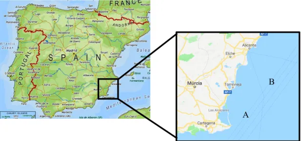
This study took place at Piscialba, Piscifactorias Albaladejo S. L., a company based in San Pedro del Pinatar, Murcia, Spain, an area known for its high number of aquaculture facilities, and therefore, for its large annual production. Piscialba is a company dedicated to the fisheries and aquaculture industry, being its aquaculture sector currently focused on the grow-out of gilthead sea bream (Sparus aurata), European sea bass (Dicentrarchus labrax) and bluefin tuna (Thunnus Thynnus).
The company has a current total of thirty-seven cages at sea, divided in two different farming locations. One of them is located, approximately, three nautical miles from the San Pedro del Pinatar Port (Figure 1). It is composed of twenty-seven cages, being three of them currently used for tuna grow-out and the remaining, in no specific ratio, in the grow-out of sea bream and sea bass. The other facility is located three nautical miles from the Alicante region (Figure 1). It is composed by ten cages and it is dedicated, only, to the grow-out of sea bream and sea bass, with, again, no specific ratio.
2.2 Practical experience of the activities of a cage farm
The first part of this study was focused on learning the daily activities performed for the functionality of a cage fish farm to understand in this specific situation all the procedures that should be taken in account in the adaptation of the model. Several tasks were performed during the experiment, such as feeding predictions, nets management,
A
B
Figure 1 – Approximated location of the two farming facilities. A-Facility near San Pedro and B- Facility near Alicante.
12 feeds management, material management (different sizes of ropes, buoys, towers, etc.). Other practical tasks and skills such as, preparation of the daily amount of feed, loading techniques of the feeds into the different boats, feeding techniques used by the company (hand feeding vs mechanical feeding), preparation of the fish feed the tunas, machine operation (different mechanical feeders, different machines present on the boats), cage sampling, fish transferences, cage fisheries, medicinal baths, net exchanging, introduction of new batches to the cages and overall cage maintenance were also acquired.
During this period, it was also observed how different parameters can be difficult to collect on site. It was observed if, among others, environmental parameters, such as temperature, currents and wind, behaviour parameters, amount of feed provided, mortality and predator presence can actually be easily collected by the farmers in a daily base situation and what was the best method of collection.
2.3 Optimisation of algorithms to predict fish biomass in cages
We analysed the moving average of the estimated biomass in order to obtain the deviation from the estimation and the total of harvested biomass. After getting the deviations for the biomass estimation, the parameters such as mortality, density, number of individuals and mean weight were analysed. Through the analyse of these results we were able to understand which of these parameters are influencing the biomass estimation.
2.3.1Samplings
The first harvest done in each cage was considered a sampling for parameters such as the number of fish, the mean weight and the biomass estimations. These harvests were performed at night. A net with an open bottom was casted around half of the cages area. By closing the net, the fish were gathered in a confined area closer to the boat. A spoon net was then used to collect the fish from the cage onto the boat. The desired amount of fish would be placed in large ice boxes and transported to the port. From there, fish were transferred into a truck and taken to the company facilities to be processed. There, the fish was selected by weight classes and separated in ice boxes ready for the market. The data collected in this process, regarding the mean weight and the number of fish, was used to adjust the estimations on this study.
13 Data for mortality was recorded every two days. Divers would collect the deceased individuals from within the cages and register its number.
Moving average of the estimated biomass, density, estimated number of fish, estimated mean weight are values provided by the software.
The studied cages have already been completely harvested so that values of total harvested biomass, total number of fish harvested and mean weight of the harvested fish can be used. It was analysed the data from a total of seven cages, being five from the facility located in Murcia and the remaining two from the facility located in Alicante. Sea bream cages sampled in this study are cages 06, 09, 11 and 110. The first three belong to the facility in Murcia and the last, cage 110, belongs to the facility in Alicante. Sea bass cages are cages 03, 14 and 109. Cage 109 belongs to the Alicante facility and the remaining two belong to the facility in Murcia.
2.3.2Data treatment
There were analysed two different time periods in the calculations of the moving average of the estimated biomass, a parameter that uses the estimation of biomass (feed fed/SFRmodel) and calculates its mean in a certain time period. The two time periods tested
are one of fourteen days (MA14) and the other of thirty days (MA30) prior to the first
harvest, with the final purpose of understanding which of them would provide a better biomass estimation. The deviation between the values for the different time periods was then calculated against the values of the total harvested biomass for each cage. Mortality and Density are others of the parameters analysed in this study. Both of them being studied using as the mean of the fifteen days prior to the first harvest. Finally, the predicted number and mean weight of fish were also studied. Both of these parameters was calculated for the day of the first harvest for each of the studied cages. The deviation of this value was then calculated against the total number of fish harvested and the mean weight of the harvested fish, respectively, at the end of all the harvests. The deviation between the estimated values and the observed provided the error of the model in use.
The data was treated using the Yellowfin software. Yellowfin is a tool used in analytics and business intelligence reports, that allows the storage of data and to rapidly model, prepare, and reuse data for analysis using pre-built or custom transformations. This is the software used by Aquanetix, which facilitates the use of data and prevents
14 errors when dealing with the transference of these data. Also, Excel was used for the calculations of the deviations.
15
3 Results
16 3.1Moving Average of Estimated Biomass
The moving average of the estimated biomass was calculated using two different time periods. The one currently used by the Aquanetix software at fourteen days and a new one at thirty days, prior to the first harvest. The results for this parameter are presented for each cage separately for a better understanding of the effect of the two different time periods tested.
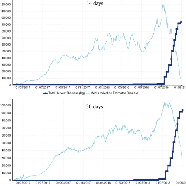
3.1.1 Cage 03 (L1794PCM)
14 days
30 days
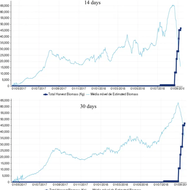
Figure 2 - Graphic representation of the Moving average of Estimated Biomass at first harvest (kg) and the Total Harvest Biomass (Kg) in cage 03 (L1794PCM) for the two time periods tested.
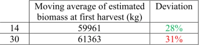
17 Cage 03, a sea bass cage containing the batch with the code L1794PCM, was first harvested in 23/08/2018 and the last harvest occurred in 09/09/2018, comprising a period of 17 days. After the last harvest a biomass total of 46884 kg had been captured. From the tested periods for the moving average, the one that estimated the closest relationship with the total biomass harvested was the MA14 (moving average using the last 14 days)
days with an estimation of 59961 kg, having a 28% overestimation, being the most distant estimation the Ma30 (moving average using the last 30 days) with 61363 kg and an
overestimation of 31% (Figure 2/ Table 1). Both of the estimations were found to be above the 10% deviation that we consider as reasonable.
Table 1 - Moving average of estimated biomass at first harvest (kg) for the two time periods tested and the respective deviation against the total harvested biomass. In green is represented the best result and in red the worst.
Moving average of estimated
biomass at first harvest (kg) Deviation
14 59961 28%
18 3.1.2 Cage 06 (D1691PCM)
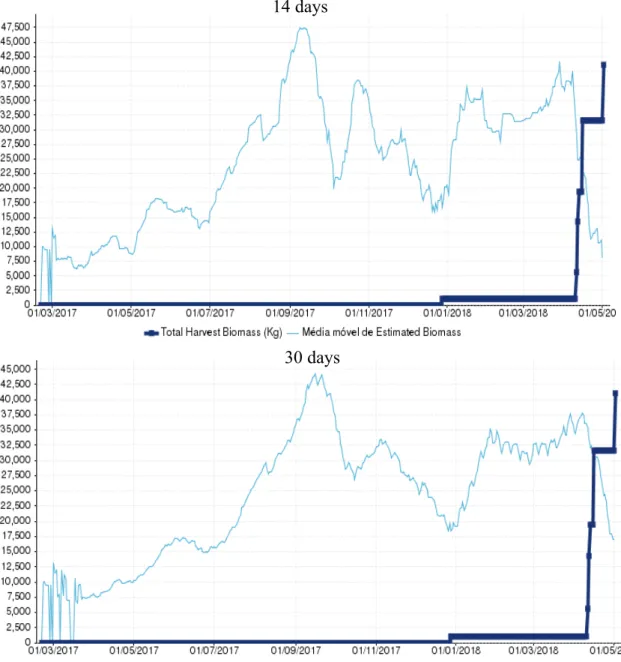
Cage 06, a sea bream cage containing the batch with the code D1691PCM, was first harvested in 28/05/2018 and the lastly in 20/06/2018, comprising a period of 23 days.
14 days
30 days
Figure 3 - Graphic representation of the Moving average of Estimated Biomass at first harvest (kg) and the Total Harvest Biomass (Kg) in cage 06 (D1691PCM) for the two time periods tested.
19 At the end of all the harvests a biomass total of 56156 kg had been captured. From the tested periods for the moving average, MA30 showed the closest relationship with the total
biomass harvested with an estimation of 53951kg and an underestimation of only 4%, being the most distant estimation the one provided by MA14 of 60141 kg and an
overestimation of 7% (Figure 3/ Table 2). The estimations provided by MA14 and MA30
were both found to be within the 10% deviation considered reasonable.
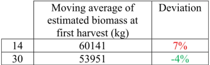
Table 2 - Moving average of estimated biomass at first harvest (kg) for the two time periods tested and the respective deviation against the total harvested biomass. In green is represented the best result and in red the worst.
Moving average of estimated biomass at first harvest (kg) Deviation 14 60141 7% 30 53951 -4%
20 3.1.3 Cage 09 (D1687PCM)
Cage 09, a sea bream cage containing the batch with the code D1687PCM, was first harvested in 11/04/2017 and the last harvest occurred in 01/05/2018, comprising a period of 20 days. After the last harvest a biomass total of 41099 kg had been captured. MA30 was proven to be the one with a closest estimation to the total biomass harvested
with 35318kg and an underestimation of 14%, being the most distant estimation the one provided by MA14 with 29014 kg and an underestimation of 29% (Figure 4/ Table 3).
14 days
30 days
Figure 4 - Graphic representation of the Moving average of Estimated Biomass at first harvest (kg) and the Total Harvest Biomass (Kg) in cage 09 (D1687PCM) for the two time periods tested.
21 Both were found to be underestimations outside of the 10% deviation considered reasonable.
Table 3 - Moving average of estimated biomass at first harvest (kg) for the two time periods tested and the respective deviation against the total harvested biomass. In green is represented the best result and in red the worst.
3.1.4 Cage 11 (D1689PCM) Moving average of estimated biomass at first harvest (kg) Deviation 14 29014 -29% 30 35318 -14% 14 days 30 days
Figure 5 - Graphic representation of the Moving average of Estimated Biomass at first harvest (kg) and the Total Harvest Biomass (Kg) in cage 11 (D1698PCM) for the two time periods tested.
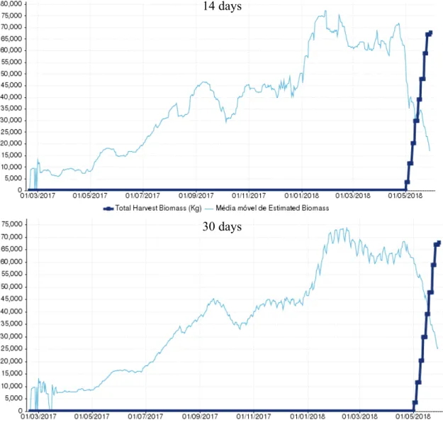
22 Cage 11, another sea bream cage containing the batch with the code D1698PCM, had the first harvest made in 02/05/2018 and the last occurred in 29/05/2018, comprising a period of 27 days. After the last harvest a biomass total of 67898 kg had been captured. MA30 showed, once again, to be the one with the closest estimation of the total biomass
harvested with 59483 kg and an underestimation of 12%, being the most distant estimation the one provided by MA14 with 47472 kg and an underestimation of 30%
(Figure 5/ Table 4). Once again, both are found to be underestimations outside of the 10% deviation that we considered reasonable.
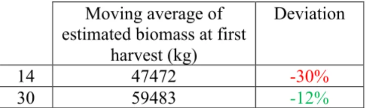
Table 4 - Moving average of estimated biomass at first harvest (kg) for the two time periods tested and the respective deviation against the total harvested biomass. In green is represented the best result and in red the worst.
Moving average of estimated biomass at first
harvest (kg)
Deviation
14 47472 -30%
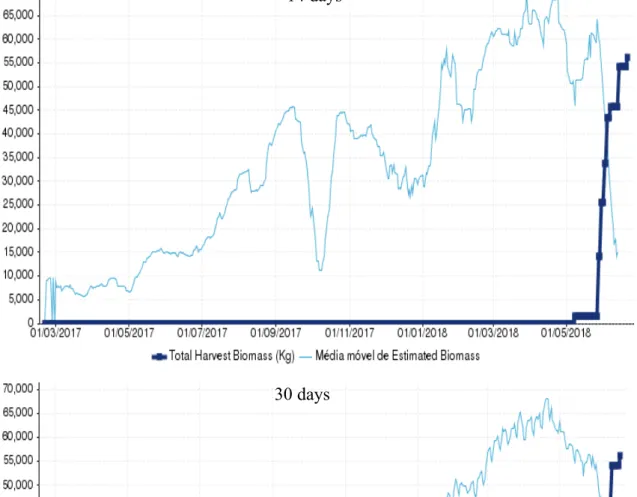
23 3.1.5 Cage 14 (L1792PDM)
Cage 14, a sea bass cage containing the batch with the code L1792PCM, was first harvested in 10/07/2018 and lastly in 28/08/2018, comprising a period of 49 days. After the last harvest a biomass total of 94366 kg had been captured. From the tested periods for the moving average, MA30 was the one with the closest relationship to the total
biomass harvested with 99920 kg and an overestimation of 6%, being MA14 the one most
distant with 110842 kg and an overestimation of 17% (Figure 6/ Table 5). MA30 was
14 days
30 days
Figure 6 - Graphic representation of the Moving average of Estimated Biomass at first harvest (kg) and the Total Harvest Biomass (Kg) in cage 14 (L1792PCM) for the two time periods tested.
24 found to be within the 10% deviation considered reasonable, wile MA14 was once again
found above it.
Table 5 - Moving average of estimated biomass at first harvest (kg) for the two time periods tested and the respective deviation against the total harvested biomass. In green is represented the best result and in red the worst.
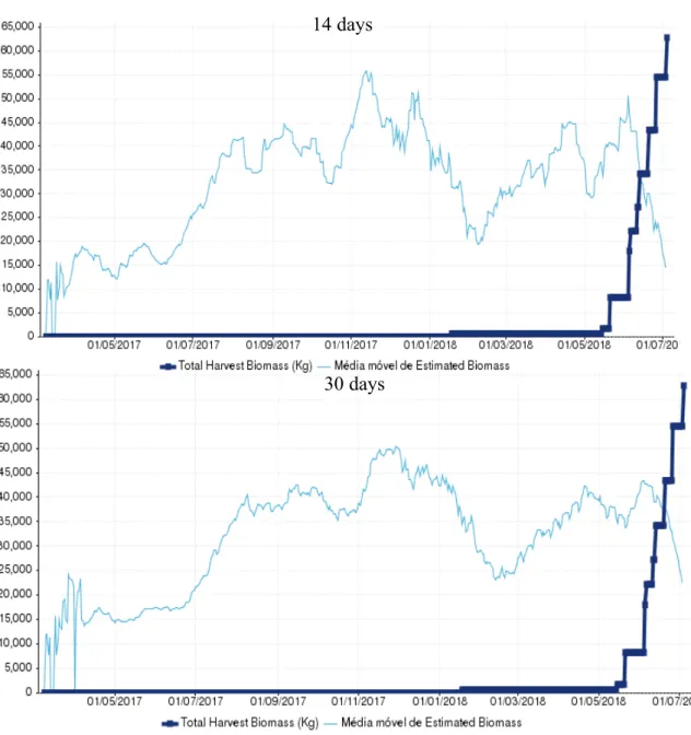
3.1.6 Cage 109 (L1686PCM)
Moving average of estimated
biomass at first harvest (kg) Deviation
14 110842 17%
30 99920 6%
14 days
30 days
Figure 7 - Graphic representation of the Moving average of Estimated Biomass at first harvest (kg) and the Total Harvest Biomass (Kg) in cage 109 (L1686PCM) for the two time periods tested.
25 Cage 109, another sea bass cage containing the batch with the code L1686PCM, was first harvested in 21/05/2018 and the last harvest occurred in 25/06/2018, comprising a period of 35 days. After the last harvest a biomass total of 62846 kg had been captured. This cage showed the highest deviation between the total biomass harvested and both MA14 and MA30, with MA14 being the closest with 40848 kg and an underestimation of
35%, wile MA30 estimated 33828kg with an underestimation of 46% (Figure 9/ Table 8).
Both were found to be way above the 10% deviation that we consider reasonable.
Table 6 - Moving average of estimated biomass at first harvest (kg) for the two time periods tested and the respective deviation against the total harvested biomass. In green is represented the best result and in red the worst.
Moving average of estimated biomass at first
harvest (kg)
Deviation
14 40848 -35%
26 3.1.7 Cage 110 (D1688PCM)
Cage 110, a sea bream cage containing the batch with the code D1688PCM, was first harvested in 18/01/2018 and the last harvest occurred in 10/07/2018, comprising the longest harvest period of all the studied cages with 173 days. After the last harvest a biomass total of 71692 kg had been captured. In this cage, MA30 provided the closest
estimation of the total biomass with 57064 kg and an underestimation of 20%, being MA14 not far behind with an estimation of 53591 kg and an underestimation of 25%
14 days
30 days
Figure 8 - Graphic representation of the Moving average of Estimated Biomass at first harvest (kg) and the Total Harvest Biomass (Kg) in cage 110 (D1688PCM) for the two periods tested.
27 (Figure 10/ Table 9). Both were found to be outside of the 10% deviation considered reasonable.
Table 7 - Moving average of estimated biomass at first harvest (kg) for the two time periods tested and the respective deviation against the total harvested biomass. In green is represented the best result and in red the worst.
In Table 8 we can see that the use of MA30 when calculating the moving average
of the estimated biomass proved, in the majority of the cages, to be the one with the best results. Although it was still not able to deliver, in the majority of the cages, an estimation inside of the 10% interval considered reasonable.
Table 8 - Moving average of estimated biomass at first harvest (kg) for the two periods tested and the respective deviation against the total harvested biomass for all the tested cages. In green is represented the best result and in red the worst.
Moving average of estimated biomass at first
harvest (kg)
Deviation
14 54,730 -25%
30 57,064 -20%
Cage Batch Code 14 days period estimation Deviation from the 14 days estimation against the total harvested biomass 30 days period estimation Deviation from the 30 days estimation against the total harvested biomass Total harvested biomass (kg) 03 L1794PCM 59961 28% 61363 31% 46884 06 D1691PCM 60141 7% 53951 -4% 56156 09 D1687PCM 29014 -29% 35318 -14% 41099 11 D1689PCM 47472 -30% 59483 -12% 67898 14 L1792PDM 110842 17% 99920 6% 94366 109 L1686PCM 40848 -35% 33828 -46% 62846 110 D1688PCM 53591 -25% 57064 -20% 71692
28 3.2 Mortality
Cage 14 (L1792PCM) showed the lowest mortality rate, in this period, with a total of 50 deceased fish, comprising only 0.01% mortality in the cage (Table 9). On the other hand, cage 107 (L1684PCM + L1683PCM) showed the highest mortality rate, with a total of 320 deceased fish, comprising 0.17% mortality in the cage (Table 9).
The cages that scored in between these values can be seen bellow, in table 9, and are represented in the colour gradient according to their difference between he lowest value (in green) and the highest value (in red).
Table 9 - Total number of deceased individuals in a period of fifteen days prior to the first harvest and the correspondent mortality percentage in the cage. In green is represented the lowest percentage between the cages and in red the highest. The values between are represented in different colours according the gradient between the lowest and higher values being the lowest in green and the highest in red.
3.3 Density
Cage 09 (D1687PCM) showed the lowest density with a total of 7.57 kg/m3 (Table
10). On the other hand, cage 14 (L1792PCM) showed the highest density with a total of 14.90 kg/m3 (Table 10).
The cages that scored in between these values can be seen bellow, in table 10, and are represented in the colour gradient according to their difference between the lowest value (in green) and the highest value (in red).
Cage Batch Code
Mortality in the 15 days prior to the
first harvest
Mortality in the 15 days prior to the first harvest (%) 03 L1794PCM 82 0.07 06 D1691PCM 170 0.09 09 D1687PCM 70 0.07 11 D1689PCM 134 0.07 14 L1792PDM 55 0.01 109 L1686PCM 615 0.42 110 D1688PCM 145 0.06
29 Table 10 - Density (kg/m3) in the day prior to the first harvest for each studied cage. In green is represented the lowest density value between the cages and in red the highest. The values between are represented in different colours according to the gradient between the lowest and higher values, being the lowest in green and the highest in red.
3.4 Number of fish
When it comes to the number of fish, cage 109 (L1686PCM) showed the lowest deviation from the total number of fish harvested with an underestimation of 7%, while the highest deviation was found in cage 06 (D1691PCM) with an overestimation of 49% (Table 11).
Cage Batch Code Density (kg/m3)
3 L1794PCM 8.69 6 D1691PCM 13.71 9 D1687PCM 6.85 11 D1689PCM 12.70 14 L1792PDM 17.76 109 L1686PCM 9.71 110 D1688PCM 14.09
30 Table 11 - Predicted number of fish at first harvest and total number of fish harvested for each of the studied cages. The deviation between these two values is represented in a colour scale were those closest to zero appear in a whitish colour, the ones representing an overestimation appear as green and the ones representing an underestimation appear as red.
3.5 Mean weight
The analyses of the mean weight found that the estimation for cage 14 (L1792PCM) showed the lowest deviation from the mean weight of the harvested fish, with an underestimation of 2%, while the highest deviation was registered for cage 110 (D1688PCM) with an underestimation of 45% (Table 12).
Cage Batch Code
Predicted nº of Fish at first harvest Total nº of fish harvested Deviation 03 L1794PCM 121569 112940 8% 06 D1691PCM 177827 119117 49% 09 D1687PCM 94516 84943 11% 11 D1689PCM 179130 151698 18% 14 L1792PDM 268627 224966 19% 109 L1686PCM 142129 152374 -7% 110 D1688PCM 204401 151104 35%
31 Table 12 - Estimated mean weight (g) and harvested mean weight (g) for each of the studied cages. The deviation between these two values is represented in a colour scale were those closest to zero appear in a whitish colour, the ones representing an overestimation appear as green and the ones representing an underestimation appear as red.
Table 13, bellow, provides an overall look at all of the parameters analysed for each cage. This facilitates the analysis when looking for patterns that can help understanding the reason for the deviations found in biomass estimation
Cage Batch Code
Estimated mean weight (g) Harvested mean weight (g) Deviation 3 L1794PCM 493.2 415.1 19% 6 D1691PCM 338.2 471.4 -28% 9 D1687PCM 307 483.8 -37% 11 D1689PCM 256 447.6 -43% 14 L1792PDM 412.6 419.5 -2% 109 L1686PCM 287.4 412.4 -30% 110 D1688PCM 262.2 474.5 -45%
33
Table 13 - Overall results for all of the parameters analysed for each of the studied cages. The deviation between for the values of the moving average of the estimated biomass, the number of fish and the mean weight is represented in a colour scale were those closest to zero appear in a whitish colour, the ones representing an overestimation appear as green and the ones representing an underestimation appear as red. The values for duration of the harvest period, mortality and density are represented in different colours according to the gradient between the lowest and higher values, being the lowest in green and the highest in red.
Ca ge Ba tc h C od e 1º h ar ve st La st h ar ve st Du ra ti on 14 d ays e st im at ion De vi at io n f ro m t h e 14 d ay s 30 d ays e st im at ion De vi at io n f ro m t h e 30 d ays To ta l h ar ve st ed b io m as s (k g) Mo rt al it y Mo rt al it y (% ) De n si ty ( k g/ m 3) Pr ed ic te d n º o f Fi sh To ta l n º of f is h h ar ve st ed De vi at io n Es ti m at ed m ea n w ei gh t (g ) Ha rv es te d m ea n w ei gh t (g ) De vi at io n 03 L1794PCM 23/08/18 09/09/18 17 59961 28% 61363 31% 46884 82 0,07% 8,69 121569 112940 8% 493.2 415.1 19% 06 D1691PCM 28/05/18 20/06/18 23 60141 7% 53951 -4% 56156 170 0,10% 13,71 177827 119117 49% 338.2 471.4 -28% 09 D1687PCM 11/04/18 01/05/18 20 29014 -29% 35318 -14% 41099 70 0,07% 6,85 94516 84943 11% 307.0 483.8 -37% 11 D1689PCM 02/05/18 29/05/18 27 47472 -30% 59483 -12% 67898 134 0,07% 12,70 179130 151698 18% 265.0 447.6 -41% 14 L1792PDM 10/07/18 28/08/18 49 110842 17% 99920 6% 94366 55 0,02% 17,76 268627 224966 19% 412.6 419.5 -2% 109 L1686PCM 21/05/18 25/06/18 35 40848 -35% 33828 -46% 62846 615 0,43% 9,71 142129 152374 -7% 287.4 412.4 -30% 110 D1688PCM 18/01/18 10/07/18 173 53591 -25% 57064 -20% 71692 145 0,07% 14,09 204401 151104 35% 262.2 474.5 -45%
34
4.Discussion
35 Cage 09, 11 and 110, all sea bream cages, show similar behaviour for all of the analysed parameters. All three show underestimations of the biomass values ranging from 25% to 30% for MA14 and 12% to 20% for MA30. MA30 showed the closest estimations
in all of the cages. These underestimations are probably caused by the underestimations found for the mean weight ranging from 37% to 45%, which even the overestimations of the number of fish ranging from 11% to 35% were not able to balance. The high deviations of the mean weight estimation surpass the ones found by Tran-Duy et al., (2005), of -0.8%, found for rainbow trout. To my knowledge, there are not many studies made on the biomass estimation, and so, it was difficult to find values to have as a baseline. The underestimations for the mean weight suggests that these cages are currently being under fed, most likely, due to a fault on the feeding model which is probably overestimating the SFR. Among the studied sea bream cages, cage 06 was the only to show an overestimation of the biomass of 7% for MA14 and an underestimation
of 4% for MA30. With both estimations being within the 10% deviation considered
reasonable, the estimations are considered to be accurate. However, cage 06 follows the same pattern of the others sea bream cages above were it is found a high underestimation of the mean weight at 28% and a high overestimation of the number of fishes at 49%. Meaning that, the values estimated for the mean weight and for the number of fish, in this cage, were able to balance each other and thus resulting in an accurate estimation. So, in reality, the data for cage 06 suggests that these cage is also being under fed, most likely, due to a fault on the feeding model which is probably overestimating the SFR. Making this a common fact to all of the sea bream cages studied. Mortality ranged from 0.07% to 0.43% and showed to have no influence in the biomass deviation for these cages. The values for density ranged from 6.85 kg/m3 to 14.09 kg/m3 and are all within the common interval used in the industry. Although this interval can be found in literature to be of a maximum of approximately 40kg/m3, for both sea bass and sea bream (Di Marco et al., 2008; Person-Le Ruyet and Le Bayon, 2009; Baldwin, 2010) in the aquaculture industry it is common for this value to not exceed the 15 kg/m3. Indicating that density had no influence the biomass estimation.
The sea bass cages, 03, 14 and 109, present different results for each of them. Cage 03 shows an overestimation for the biomass estimations of 28% for MA14 and 31%
for MA30. This overestimation is due to the overestimation of both the number of fish at
8% and the mean weight at 19%. Suggesting that the cage is being over fed, meaning that the amount of feed provided exceeds the amount of feed that the fish are actually
36 consuming, resulting in the overestimation by the model of the mean weight and consequently the overestimation of the cages biomass. On the other hand, cage 109 showed an underestimation of the biomass estimations with 35% for MA14 and 46% for
MA30. The values for the number of fish present an underestimation of 7% which is
surprising. Parameters that affect the number of individuals, such as mortality and escapees, are know to be hard to collect accurately and end up to lead to an overestimation of the number of fish. This suggests that the number of fry stocked in this cage was in fact higher than expected. Estimations for the mean weight, on this cage, showed an underestimation of 30% and were the main reason for the biomass underestimation. Suggesting that the cage was being under fed, if we accept that the feeding model is good, or that the feeding model is overestimating the SFR. At last, cage 14 registered overestimations of 17% for MA14 and 6% for MA30. These were probably caused by the
overestimation of the number of fish at 19%. Suggesting that the registration of parameters such as mortality or escapees was poorly recorded and lead to this overestimation. The mortality percentage registered the lowest values for cages 03 and 14 of 0.07% and 0.02%, respectively. In opposition to this, cage 109 showed the highest mortality among all of the studied cages at 0.43%. Although variable, in the end mortality seemed to have no influence in the results found for the biomass estimation. Density was found to be lower for cages 03 and 109 at 8.69kg/m3 and 9.71 kg/m3, respectively. On the other hand, cage 14 registered the highest value at 17.76 kg/m3.This could be prejudicial, since high densities can cause problems in the oxygen levels and reduce the feed intake. However, in this cage the mean weight shows a low deviation of -2%. Suggesting that density had no influence in the deviations found for the biomass estimation.
One of the findings in this study regards the period used to discover the mean estimated biomass. The Aquanetix software is currently using a period of fourteen days (MA14) to calculate the moving average of the estimated biomass. However, this study
shows that MA30, the mean of the estimated biomass for a thirty days period, predicts
biomass with a smaller error (Table 8), for the majority of the studied cages. This suggests that the period used for finding the mean of the estimated biomass must be adjusted from the current period of fourteen days to a thirty days one.
Also, after analysing the results for each cage, we can see that every cage of sea bream shows an under estimation of the mean weight of fish at first harvest, which in turn leads to an underestimation of the biomass, except for cage 06 where the high