383
David Alvarenga Drumond http://orcid.org/0000-0002-5383-8566 Pesquisador
Universidade Federal do Rio Grande do Sul - UFRGS Escola de Engenharia
Departamento de Engenharia de Minas Belo Horizonte – Minas Gerais - Brasil [email protected]
Cláudio Lúcio Lopes Pinto Professor
Universidade Federal de Minas Gerais – UFMG Escola de Engenharia
Departamento de Engenharia de Minas Belo Horizonte – Minas Gerais - Brasil [email protected]
Using rodogram function
to characterize hurst
coefficient in rock profiles
Abstract
Roughness is a fundamental feature to define rock deformability and resis-tance. A detailed characterization of discontinuity surface geometry is essential for understanding some of the rock’s mechanical behaviors. Fractal geometry has been used by several authors to correlate parameters such as the Hurst coefficient for JRC (Joint Roughness coefficient) to better describe a surface geometry. Surface profiles might be characterized by a fractal dimension that represents the small scale of the geometric recurrence. In this paper, we propose to modify the methodology used to identify the Hurst coefficient incorporating the rodogram function in the JRC analysis. The proposed function is less influenced by drifting effects, and seems to be more precise than the commonly used variogram function. Robust mathematical models of spatial continuity can be a better alternative to characterize the rough-ness of rock discontinuities.
Keywords: rodogram, fractal dimension, variogram, joint roughness, Hurst coefficient.
http://dx.doi.org/10.1590/0370-44672017710099
Geosciences
Geociências
1. Introduction
Joint roughness is one of the fea-tures responsible for strength, deform-ability, water flow and other rock mass properties. According to Lee (1990), discontinuities have an important in-fluence on the deformational behavior of rock masses. Roughness directly influences the internal friction angle, dilatancy and peak shear strength. Such effects are highly dependent on the scale considered. There has been a considerable amount of research on rock roughness to understand its effects on rock deformability and strength. Raimbay et al. (2017) show that the variogram fractal dimension better describes the water and polymer
solu-tion flow in rock discontinuities. Li et al. (2017) present a fractal model for analyzing the shear behavior of large-scale opened rock joints.
The Joint Roughness Coeffi-cient (JRC) is an important parameter for estimating rock quality (Barton, 1973). This parameter is commonly obtained by, visually, comparing the discontinuity profile against standard ones. The differences between actual and JRC proposed profiles has boosted the research on statistical geometry descriptions. Fractals is one of the most important methodologies for roughness description. Methodolo-gies such as the box counting method
(Feder, 1988), variogram methodology (Orey, 1970), spectral analysis (Berry and Lewis, 1980),roughness length (Malinverno, 1990) and line scaling (Kulatilake, 1988) have been used to describe roughness profiles. Most of the relevant research studies on fractal dimension analyses have been done in the last decades of the twenty century.
Many authors have proposed s e v e r a l r e l a t i o n s h i p s a s s o c i a t -ing fractal geometry, JRC and rock roughness(ODLI NG , 1994),(X I E , 1995), (BADGE, 2002).As discussed by Lee (1990), the relationship between JRC and the Hurst coefficient can be described as the empirical equation:
JRC
= -0.87804 + 37.7844
D
- 1
0.015
- 16.9304
D
- 1
0.015
2
where D is the profile fractal dimen-sion given by D=2-H. The equation is bounded for D values between (1.0046 and 1.013).T he Hurst coefficient 0 < H < 1 characterizes the self-similari-ty of rock profiles. A higher Hurst coef-ficient indicates lower rugosity while a lower Hurst coefficient indicates higher
rugosity. Experimental variograms are a common methodology used to estimate the Hurst coefficient.
The Hurst coefficient can be rea-sonably defined for stationary fields. A stationary behavior is commonly re-lated to a stochastic process with mean and variance being constant along the
distance. However, drifting can be ob-served in most of engineering practical instances. It consists in one of the main problems in applying variogram meth-odologies to describe rugosity as much as in several other geostatistical features. Figure 1 illustrates a discontinuity pro-file obtained in a laboratory test.
384 REM: R. Esc. Minas, Ouro Preto, 71(3), 383-389, jul. sep. | 2018
Figure 1
Discontinuity profile in a laboratory test.
This profile (Figure 1) is highly af-fected by the drift effect. Alternatively, the experimental data could be turned into a stationary field using a data transformation methodology. Figure 2 demonstrates the same profile after data transformation. For
this data transformation, linear regression was made to define the mean behavior of the profile, and simple rotation of the data provided the angle of a straight line, thus producing a new stationary behavior with constant mean. However, the
mathemati-cal methodology used to obtaina stationary field might reduce the rugosity scale and its variability (Vieira et.al, 2010). Even though stationarity can be reached mathematically, small trends should be considered since it is intrinsic to engineering problems.
Figure 2
Discontinuity profile after data transformation. Note: scales used in Figure 1 and Figure 2 are not the same.
1.2 Fractal geometry
Maldebrot (1977) introduced the concept of fractal geometry and the defi-nition of “dimensions” that have been used in several areas of physics, math-ematics and engineering. A line can be entirely representedin a1-D space; an ideal plane ina 2-D and a solid, a cube for example, can be represented
by a 3-D space. Fractal dimension can be represented by a subdivision of a Euclidian dimension, and have mixed geometrical properties.
According to Kulatilake (1988), fractals can be understood as self-affined or self-similarity entities. A self-similar fractal is a geometric feature
that retains its statistical properties through various magnifications of itself. Differently, self-affined fractals change their statistical properties for different scales. It would not be reasonable to characterize rock roughness with self-similarity methodologies, due to its natural rock properties.
1.3 Generation of fractional Brownian profiles
Brownian motion profiles were cre-ated, using a constant Hurst coefficient, to compare the rodogram function estimation against the traditional variogram function.
Saupe (1988) describes several
algo-rithms for creating fractal geometries. The author discusses awell-known method to create fractional Brownian profiles called the Midpoint Displacement methodology. Thisproposition modifies the coordinates
of the line points based on a recursive function that redefines the midpoint of each sub segment. Figure 3 demonstrates the process of midpoint division. At level N=1, point 3 was created as follows:
x
(3) =
1
2
x
(1) +
x
(2)
y
(3) =
1
2
y
(1) +
y
(2)
+ D
1(2)
(4)
(6) (3)
(5)
(7) where D1 is a normal random variable with mean =0 and variance =∆2
1. The following points are definedbythe recursive function:
x
(4) =
1
2
x
(1) +
x
(3)
y
(4) =
1
2
y
(1) +
y
(3)
+ D
2x
(5) =
1
2
x
(3) +
3
(2)
y
(5) =
1
385
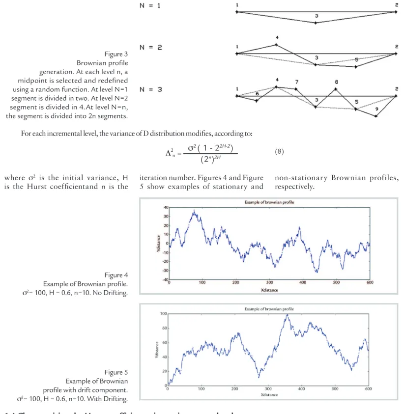
Figure 3 Brownian profile generation. At each level n, a midpoint is selected and redefined using a random function. At level N=1 segment is divided in two. At level N=2 segment is divided in 4.At level N=n, the segment is divided into 2n segments.
For each incremental level, the variance of D distribution modifies, according to:
Δ
2 n=
(2
n)
2Hσ
2( 1 - 2
2H-2)
(8)
where σ2 is the initial variance, H
is the Hurst coefficientand n is the
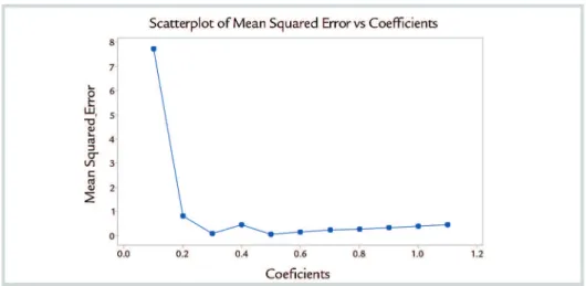
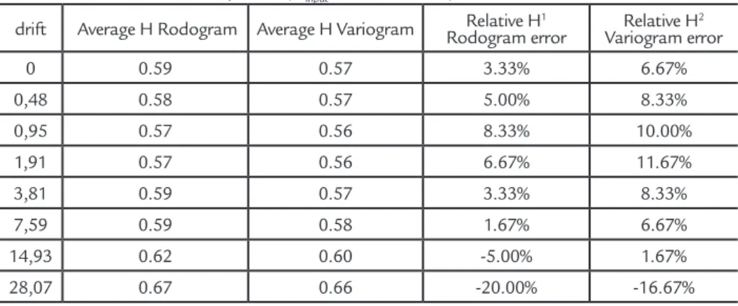
iteration number. Figures 4 and Figure 5 show examples of stationary and
non-stationary Brownian profiles, respectively.
Figure 4 Example of Brownian profile.
σ2= 100, H = 0.6, n=10. No Drifting.
Figure 5 Example of Brownian profile with drift component.
σ2= 100, H = 0.6, n=10. With Drifting.
1.4 Characterizing the Hurst coefficient using variogram and rodogram
Variogram can be defined as the expected value of the squared differ-ence of regionalized random variables
E[(Zi-Zi+h)2]/2. According
(KULATI-LAKE, UM e PAN, 1998) one can estimate the Hurst coefficient using a
variogram function with the following relationship:
2
γ
(x,h)
→h=0=
K
vh
2HwhereKv is a coefficient of proportional-ity, H is the Hurst coefficient and h, as in the classical geostatistic, is the distance vector between two samples. The Hurst component can be obtained by linearizing the log-log plot (log (2γ (x,h)) and log (h)).
The Rodogram function is a robust estimator that is less susceptible to non-stationary effects. According to Goovaerts (1997), this robust estimatormay provide a clearer description of spatial continuities revealing their ranges and anisotropies
much better than the traditional vario-gram. This article proposes to estimate the Hurst coefficient using the Rodogram function defined as E[(|Zi-Zi+h|)0.5]/2, where
Z is the regionalized random variable, modifying Equation 9 into:
(9)
(10)
386 REM: R. Esc. Minas, Ouro Preto, 71(3), 383-389, jul. sep. | 2018
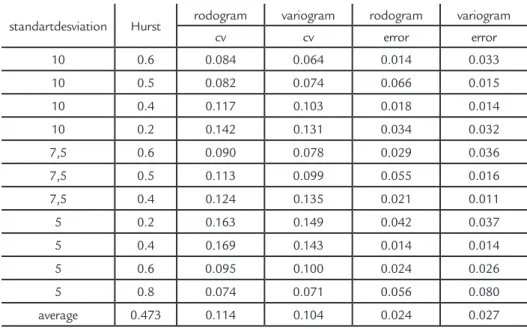
Figure 6 shows the mean square error versus exponents in equation
10. It seems that the choice of coef-ficient of 0.5 is a better alternative to
determine the Hurst coefficient using Rodogram function.
Figure 6
Scatterplot of mean squared error versus coefficients for a Hurst coefficient of 0.9 previously determinated.
2. Methodology
To compare the variogram and rodogram methodologies, Brownian profiles have been generated. Table 1 presents the parameters used to gener-ate a stationary Brownian profile using an initial horizontal base line. For the non-stationary profile generation, the y
coordinate of the end-point of the origi-nalbaseline was modified according to a chosen drifting angle. A drifting angle in a Brownian profile can be simply defined as the arctangent of the difference in yfinal and ystart divided by the difference of xfinal and xstart. An initial Hurst
coef-ficient of 0.6 was used as a standard value. The objective here is to estimatethe Hurst coefficient on this profile using traditional variogram and rodogram methodologies. Python programming was used to gener-ate the Brownian profiles according to the same algorithm showed in section 1.3.
Brownian Profile Parameters
(x,y) start (0.0)
(x,y) final (without drifting) (600.0)
Hurst coefficient 0.6
Initial st deviation 10
Table 1
Brownian Profile parameters. Hurst coefficient was imputed as constant.
Variogram and rodogram log plots were used to define the best lin-ear fitting points as shown in Figure 7.Hurst coefficients were estimated
using 5 lags of 10 unities of size. Ac-cording to Kulatilake (1988), differ-ent lagsizes cause differences in the Hurst estimator; therefore, a standard
parameter for spatial continuity func-tions was used for better comparison between the rodogram and variogram methodologies.
Figure 7
Spatial continuity
functions log plot –(Seven points).
Groups of 10 Brownian profiles-generated with the same imposed Hurst coefficient, the same variability and the same drifting angle (Hinput =0.6 and σ =10) were used to compute the statistics of the estimated Hurst coefficient. The estimation
error was calculated for both spatial conti-nuity functions (rodogramand variogram). The Hurst coefficient average error for different drift values were calculated as the difference between the expected value, defined by the mean of estimated values,
and the true value, previously used for creating the roughness profiles.
387
used in these plots.
Finally, the error was graphically
analyzed for different Hurst coefficients for a non-drifting surface, to compare
the differences between thevariogram androdogram methodologies.
3. Results and discussion
The averages of the Hurst coeffi-cient calculated for different driftsare presented in Table 2. The drifting
angles were obtained by increasing the n-point vertical distance using a factor of 2. The original profile
gen-eratedwas obtained using a constant Hurst coefficient of 0.6.
Hurst component (Hinput =0,6 and σ =10) x estimation error
drift Average H Rodogram Average H Variogram Rodogram errorRelative H1 Variogram errorRelative H2
0 0.59 0.57 3.33% 6.67%
0,48 0.58 0.57 5.00% 8.33%
0,95 0.57 0.56 8.33% 10.00%
1,91 0.57 0.56 6.67% 11.67%
3,81 0.59 0.57 3.33% 8.33%
7,59 0.59 0.58 1.67% 6.67%
14,93 0.62 0.60 -5.00% 1.67%
28,07 0.67 0.66 -20.00% -16.67%
Table 2 Hurst coefficient error (Hinput =0.6 and σ =10) for different drift values.
The average error of the Hurst coefficientsfor eachdrift are presented in Figures 8,9, and 10. The rodogram estimator presents smaller errors than
the variogram estimator for drift angles under approximately 10°.Higher drifts, where the variogram can be considered a better estimator are not usually found
in rugosity profiles. It should also be pointed out that for drift angles over around 10°, the error increases rapidly for both methodologies.
Figure 8 Average Error of Hurst coefficient vs drift. Hurst coefficient 0.6 and σ=10.
Figure 9 Average Error of Hurst coefficient by drift. Hurst coefficient 0.7 and σ=10.
388 REM: R. Esc. Minas, Ouro Preto, 71(3), 383-389, jul. sep. | 2018
Figure 10
Average Error of Hurst coefficient by drift. Hurst coefficient 0.8 and σ=10.
When a stationary problem has been considered, the variogram is a more precise estimator than the
rodo-gram (average rodorodo-gram error is less than variogram average error), but less accurate (the rodogram coefficient of
variation is greater than the variogram), as shown in Table 3 .
standartdesviation Hurst rodogram variogram rodogram variogram
cv cv error error
10 0.6 0.084 0.064 0.014 0.033
10 0.5 0.082 0.074 0.066 0.015
10 0.4 0.117 0.103 0.018 0.014
10 0.2 0.142 0.131 0.034 0.032
7,5 0.6 0.090 0.078 0.029 0.036
7,5 0.5 0.113 0.099 0.055 0.016
7,5 0.4 0.124 0.135 0.021 0.011
5 0.2 0.163 0.149 0.042 0.037
5 0.4 0.169 0.143 0.014 0.014
5 0.6 0.095 0.100 0.024 0.026
5 0.8 0.074 0.071 0.056 0.080
average 0.473 0.114 0.104 0.024 0.027
Table 3
Rodogram and variogram errors and coefficient of variation for different standard deviations, and inputHurst coefficients. No drift has been considered.
Figure 11 presents the Hurst coef-ficient error for the different profiles generated. It seems that the average error of linear estimators (variogram and rodo-gram) are only deslocated by a constant defined by the exponent of the spatial
continuity function as demonstrated in Figure 10. As discussed by Kulatilake (1988), the error presented by the vario-gram methodology increases as the Hurst coefficient increases. Rodogram method-ology seems to be better defined for high
Hurst coefficient values and lower drifts, less than 10 degrees. Considering that rock roughness profiles can be defined at these terms, the Rodogram methodology can be a better alternative for describing rock mass discontinuity roughness.
Figure 11
389
4. Conclusion
In this study, the spatial continu-ity function rodogram was proposed to estimate the Hurst coefficient of rock discontinuity roughness profiles instead of the variogram commonly used. Brownian profiles were created imposing a Hurst coefficient which has been forward esti-mated using models of spatial
continu-ity. Rodogram methodologies presented errors lower for small drifts and small fractal dimensions when compared to variogram methodologies. Variograms were less accurate than rodograms when small drifts are considered (lower than 10°). For higher drift values, neither the variogram or the rodogram
methodol-ogy presented good results for Hurst parameter determination. When no drift was considered, both the rodogram and variogram essentially presented the same error for a Hurst coefficient lower than 0.6. Variogram and rodogram methodolo-gies failed to describe the Hurst coefficient for profiles presenting higher roughness.
References
BADGE, M. N. E. A. Rock mass characterization by fractal dimension. Engineering Geology, v. 63, p. 141-155, 2002.
BARTON, N. Review of a new shear strengh criterion for rock joints. Engineering Geology, v. 7, p. 287-332, 1973.
BERRY, M. V., LEWIS, Z. V. On the Weirstrass-Mandelbrot fractal function. Proceedings of the Royal Society of London A. Mathematical, Physical and
Engineering Sciences, v. 370, 1980.
FEDER, J. Fractals. New York: Plenum Press, 1988.
GOOVAERTS, P. Geostatistics for natural resources evaluation. [S.l.]: Oxford University Press on Demand, 1997.
KULATILAKE, P. H. S. W., UM, J., PAN, G. Requirements for accurate quantifica-tion of self-affine roughness using the variogram method. International journal of solids and structures, p. 4167-4189, 1998.
LEE, Y.-H. E. A. The fractal dimension as a measure of the roughness of rock discon-tinuity profiles. International Journal of Rock Mechanics and Mining Sciences & Geomechanics Abstracts, v. 27, 1990.
LI, Y. et al. A Fractal model for the shear behaviour of large-scale opened rock joints.
Rock Mechanics and Rock Engineering, 50, p.67-79, 2017.
MALINVERNO, A. A simple method to estimate the fractal dimension of a self affine series. Geophysical Research Letters, v. 17, p. 1953-1956, 1990.
MANDELBROT, B. B. Fractals. [S.l.]: John Wiley & Sons, Inc, 1977.
MATSUSHITA, M., O. S. On the self-affinity of various curves. Journal of the Physi-cal Society of Japan, p. 1489-1492, 1989.
ODLING, N. E. Natural fracture profiles, fractal dimension and joint roughness coe-fficients. Rock mechanics and rock engineering, v. 27, p. 135-153, 1994.
OREY, S. Gaussian sample funcitons and housdorff dimension of level crossings x. Wahrsheninkeits theorie verw. Gebierte, p. 249-256, 1970.
RAIMBAY, A. et al. Fractal analysis of single-phase water and polymer solution flow at high rates in open and horizontally displaced rough surfaces. International Journal of Rock Mechanics & Mining Sciences, 92, p.54-71, 2017.
SAUPE, D. Algorithms for random fractals. New York: Springer, 1988.
VIEIRA, et al. Detrending non stationary data for geostatistical applications. Bragan-tia, Campinas, v. 69, 2010.
XIE, H. Fractal estimation of joint roughness coefficients. Chinese Science Abstracts, p. 55, 1995. (Series B).