v.14, n.3, p.253–260, 2010
Campina Grande, PB, UAEA/UFCG – http://www.agriambi.com.br Protocolo 149.07 – 28/07/2007 • Aprovado em 10/08/2009
Determining the deficit coefficient as a function
of irrigation depth and distribution uniformity
Everardo C. M antovani1, Gregório G. Faccioli2, Brauliro G. Leal3, Luis C. Costa1, Antônio A. Soares1 & Paulo S. L. Freitas4
ABSTRACT
The present study aimed at the development of the water deficit coefficient as a function of the Christiansen uniformity coefficient and relationship between the applied water depth and that required by a given crop, taking into account that the water distribution by the sprinkler follows a normal distribution. Another objective was to compare the experimental results to those obtained through simulation with the Mantovani model. For this, the water deficit coefficients developed in this work were used, as well as the simplified coefficient that takes into account the water distribution by the sprin-kler following a uniform distribution, and finally the development of the production functions for the bean crop by using the Mantovani model. The production values simulated by the model, using the normal deficit coefficient, were always less than those simulated with the uniform deficit coefficient for all uniformity levels and all values of the crop’s maxi-mum evapotranspiration fraction restored by other sources (p). Under the conditions that this study was carried out, the use of the water deficit coefficient based on the normal distribution model did not provide a better performance of the simulation model proposed by Mantovani.
Key words: sprinkle, simulation models, bean crop
Determinação do coeficiente de déficit em função da lâmina
de irrigação e da uniformidade de distribuição
RESU M O
Os objetivos primordiais neste trabalho foram: o desenvolvimento do coeficiente de déficit em função do coeficiente de uniformidade de Christiansen e da relação entre a lâmina aplicada e a lâmina requerida pela cultura, considerando-se que a distribuição de água pelo aspersor segue a distribuição normal, e a comparação dos resultados experimentais com os resultados obtidos por meio da simulação com o uso do modelo proposto por Mantovani, utilizando-se coeficientes de déficit desenvolvido no presente estudo e o coeficiente simplificado, que considera a distribuição de água pelo aspersor, seguindo a distribuição uniforme e, por último, o desenvolvimento das funções de produção para a cultura do feijão com o modelo desenvolvido por Mantovani. Os valores do rendimento simulados pelo modelo através do coeficiente de déficit normal, foram sempre inferiores aos valores simulados com o coeficiente de déficit uniforme, para todos os níveis de uniformidade e para todos os valores da fração da evapotranspiração máxima da cultura reposta por outras fontes (p). Nas condições de realização deste trabalho, a utilização do coeficiente de déficit baseado no modelo de distribuição normal não possibilitou maior precisão na utilização do modelo de simulação proposto por Mantovani.
Palavavras-chave: aspersão, modelos de simulação, cultura do feijão
1DEA/UFV Av. P. H. Rolfs S/N, CEP 36571-000, Viçosa, MG. Fone: (31) 3899-2730. E-mail: [email protected]; [email protected]; [email protected] 2NESSA/UFS, CEP 49096-150, São Cristóvão, SE. Fone: (79) 2105-6795. E-mail: [email protected]
INTRODUCTION
Several factors regarding soil, plant and atmosphere in-teract, determining the productivity of agricultural crops. There is certainly a functional relationship among these fac-tors and crop production, characteristic of each environmen-tal condition (Frizzone, 1998).
The term production function applies generically to any relationship that characterizes the crop response to a deter-mined factor such as water, fertilizer and energy. Generally, the production functions regarding water permit an analysis of the total dry matter production or commercial matter pro-duction of the crops for transpiration, evotranspiration or quantity of water applied by irrigation. Knowing these rela-tionships is necessary to assess irrigation strategies (Manto-vani et al., 1995).
Stewart et al. (1977) reported several studies that show a linear relationship between yield reduction in crops and sea-sonal evotranspiration deficit. According to the authors, the angular coefficient (β) is a measure of the sensitivity of the crop to water deficit that differs greatly among crops and also among varieties. Although the linear relationship has repre-sented well the reduction in relative yield as a function of the relative evotranspiration deficit, the authors emphasized the need for care in extrapolating the results.
According to Hanks (1983) the problem of using the model proposed by Stewart et al. (1977) is due to the need to determine β in field experiments.
Karmeli (1978) developed a linear distribution model, making it possible to characterize sprinkler precipitation patterns, efficiency and other irrigation parameters. The model is based on the accumulated frequency curve, relat-ing the adimensionalized infiltrated water depth and the frac-tion of the area that received the water depth by a linear regression function
According to Walker (1979), by minimizing the sum of the squares of the deviations of estimated compared to ob-served findings, a straight line can be fitted to the frequency curve.
According to Anyoji (1994), when a population is nor-mally distributed, with mean and standard deviation repre-sented by µ and σ, respectively, the probability density func-tion of the populafunc-tion. The mean of the populafunc-tion is m and the deviations regarding the mean are µ±ασ, where α spec-ifies the deviation in terms of the standard deviation σ. The author reported that when the extension of the population is included between µ − 3σ and µ + 3σ, the confidence limits will be fixed at 99%.
Many statistical tests require the assumption of normali-ty. Therefore methodologies to assess whether data come from a normal distribution are necessary (Cecon, 2001).
According to Cecon (2001), by residual histogram nor-mality can be ascertained of the group of data the chi-square tests for adherence and the Kolmogorov-Smirnov and the Shapiro-Wilks tests can also be used.
According to Gomide (1976) when a postulated distribu-tion is not completely specified, that is, when parameters need to be estimated, the chi-square test for adherence is
applicable to verify the normality of the distribution, as long as the number of degrees of freedom is altered, taking into consideration the number of parameters estimated. Further-more, the parameters should be estimated by the maximum likelihood and calculated based on clustered data.
Warrick & Gardner (1983) reported that log-normal, po-tential, Beta and gamma cumulative probability density func-tions can be used to describe the irrigation efficiencies, wa-ter distribution uniformity and to characwa-terize the sprinkler precipitation patterns. In this study, mathematical consider-ations are presented for each one of these distributions.
Warrick & Gardner (1983) also presented several equa-tions that relate the Christiansen uniformity coefficient (CUC) and the distribution uniformity coefficient (CUD) with the variation coefficient, log-normal, potential, Beta and gamma cumulative probability density functions.
The objective of the present study was the development of the deficit coefficient, considering the water distribution pattern by the sprinkler as a normal model in function of the Christiansen uniformity coefficient and the relationship between the applied water depth and the water depth required by the crop. It also aimed to compare the experimental re-sults with rere-sults obtained by simulation using the model developed by Mantovani (1995) with the deficit coefficients, considering the water distribution pattern by the sprinkler as uniform and normal.
MATERIAL
AND METHODSThis study was carried out in the Department of Agri-cultural Engineering at the Federal University of Viçosa, from June to October 2001. The Derive 5.0 software was used to solve the mathematical integrations necessary for the devel-opment of the deficit coefficient. The simulations were made with a production function model developed by Mantovani et al. (1995) for the conditions of the field experiments car-ried out in 2000 and published by Faccioli (2002). The pro-duction functions for the bean crop were developed using the production function model developed by Mantovani (1995) with the deficit coefficient, considering the water distribu-tion pattern by the sprinkler as uniform and normal.
Treatments of the field experiments carried out by Faccioli (2002)
The treatments consisted of three irrigation water depths and two levels of water distribution uniformity, represented by the Christiansen uniformity coefficient (CUC). Each treat-ment or experitreat-mental plot consisted of three blocks or three replications 12 m wide and 12 m long, totaling 12 m wide and 36 m long.
The treatments were called L1A, L1B, L2A, L2B, L3A and L3B.
applied in treatment L1A, with distribution uniformity (CUC) greater than 80%. In the L2B and L3B treatments the water depths applied were, respectively, 50% and 150% of the water depth applied in the L1A treatment, with distribution uni-formity (CUC) less than 80%.
Maximum crop yield (Ymax)
According to Doorenbos & Kassam (1979), the maximum yield (Ymax) for the dry bean crop (grain), considering high-ly productive varieties adapted to the climatic conditions of the available growth period, with satisfactory water supply and high level of agricultural chemicals, under irrigated agricultural conditions, is 2,500 kg ha-1.
According to the Minas Gerais Agricultural Research Corporation (EPAMIG), the maximum yield (Ymax) for the dry bean (grain) crop, Pérola variety, for the Zona da Mata region, is 3,000 kg ha-1.
For the simulations, the maximum yield (Ymax) value con-sidered was 3,000 kg ha-1.
Deficit coefficient
To develop the deficit coefficient in function of CUC, the applied water depth (HG) and the water depth required by the crop (HR), the Christiansen uniformity coefficient (CUC) and the water deficit in the soil (HD) were determined for the cumulative probability density function of the normal distribution model.
Anyoji (1994) presented a mathematical solution of the area integrations for normal distribution. These solutions were used as support to define the water deficits in the soil (HD).
The results of the integrations of the areas defined in the graph of the cumulative probability density function for nor-mal distribution, according to Anyoji (1994) are shown as follows:
where:
σ– standard deviation
α– deviation in terms of the standard deviation
µ– mean
xi– accumulated probability density
Simulations using the model proposed by Mantovani (1995) Mantovani et al. (1995) named applied net water depth, water depth required by the crop and water deficit water depth in the soil as HG, HR and HD, respectively. According to the authors the water depth is used to compensate the water deficit in the soil or to meet the requirements of the crop, and that the deficit coefficient was defined by the ratio be-tween the water deficit (HD) and the water depth required by the crop (HR)
The production function model developed by Mantovani (1995).
where:
Y – atual yield Ymax– maximum yield
β– coefficient of sensitivity of the crop to water deficit
CDmed– seasonal mean of the deficit coefficient p – fraction of the ETmax that is the response by
other sources that are not irrigation.
According to Mantovani et al. (1995), the ratio between the deficit coefficient (Cd) and the applied water depth (HG) is a function of the CUC and can be defined for sprinkler irrigation systems.
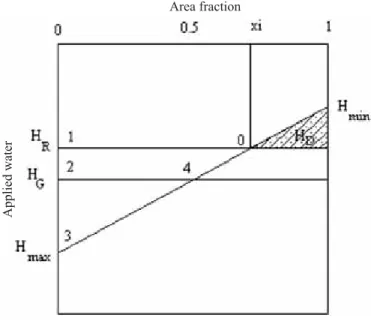
To develop the deficit coefficient, the author considered one water distribution profile by the sprinklers followed a uniform distribution (linear function) and that 50% of the area received a water depth equal or superior to the applied water depth (HG) (Figure 1).
According to Mantovani et al. (1995), one of the terms of CUC can be represented by the ratio between the sum of the deviation module in relation to the required water depth and the applied net water depth. Figure 1 shows that half the sum of the module of the deviations corresponds to the area of the triangle 2, 3, 4.
where:
CD– deficits coefficient, adimensional CUC – Christiansen uniformity coefficient
HG– applied water depth, mm; and
HR– water depth requires by the crop, mm.
(11)
( )
1 p CdY Y
1 med
max
− β
= −
(8)
( ) 2
2 e 2 . D 1 xi .
α − π σ + σ = − α
(7)
− . .
D C 1 xi
(6) 2
2 e 2 i x 1 . C
α − π σ − − µ = ⎜⎝⎛ ⎟⎠⎞
(5) 2
2 e 2 . i x C
A ..
α − π σ − σ + µ =
+ α
(4) C
B A
σ − α − π σ
= 2 xi.α..
2 e 2
B (3)
(1)
i x . 2
2
e 2 B
A +µ
α − π σ = +
(2) .
i x A
(9) R
D H H Cd=
(10)
( )
1 pCd ET
ET
1 med
max
− =
−
(12)
(
)
⎥⎥⎦ ⎤ ⎢
⎢ ⎣ ⎡
⎟ ⎟ ⎠ ⎞ ⎜
⎜ ⎝ ⎛
− −
⎥ ⎥ ⎥ ⎥ ⎥
⎦ ⎤
⎢ ⎢ ⎢ ⎢ ⎢
⎣ ⎡
− + −
= 2CUC 1
H H . 1 CUC 8 8
H H CUC 2 1 C
R G G
According to Mantovani et al. (1995), when there are no losses in irrigation, or rather, Hmax< HR, equation 13 can-not be applied, because the xi data are negative (Figure 1) and there is no negative area fraction. According to the au-thor, in this case the CD value is easily calculated as:
The simulations were carried out with the production function model developed by Mantovani et al. (1995) for the conditions of the field experiments presented in this study by Faccioli (2002), using the deficit coefficients developed for the precipitation profile of water from the sprinklers as uniform (Mantovani, 1995) and normal. As the treatments consisted of three irrigation water depths and two water dis-tribution uniformity levels, 12 simulations were made; six using the deficit coefficient developed for the uniform dis-tribution profile and six for the normal profile.
The data necessary to carry out the simulations were: maximum crop yield (Ymax), sensitivity coefficient of the crop to water deficit (β), applied water depth (HG) Christiansen uniformity coefficient (CUC), water depth required by the crop (HR) and the maximum evotranspiration fraction that is the response by other sources than irrigation (p).
The period considered to perform the simulations was from September 22 to October 28, 2000. It was decided to work with the third phenological phase of the crop, because it was the phase where irrigation was applied. If the total period of the crop development was considered, from August 10 to November 17, the total irrigation depth applied would
be smaller than the water depth required by the crop, due to rainfall during the period prior to the irrigations.
Linear transformation of the model proposed by Mantovani et al. (1995)
It was only possible to perform the simulations using a period of the total crop cycle because, mathematically, the model proposed by Mantovani (1995) is a linear transforma-tion. A function is a linear transformation when
f (0) = 0; f(x+y) = f(x) + f(y); and f(Kx) = K.f(x), K e R.
Considering the model developed by Mantovani (1995), presented in Eq. 11, some mathematical substitutions were made, to demonstrate that the function is a linear transfor-mation
where:
a, β ε R – constant Cd’ – Cdmed.(1-p) ε R
f – Y/Ymaxε R
Substituting the considerations presented previously in Eq. 10, we have
where we have
Equation 25 is a function of the F(x) = aX type. So: F (0) = 0; F (x1+x2) = F(x1) + F(x2); and F (Kx) = K.f(x).
For any x1, x2ε R and K constant, the production function developed by Mantovani et al. (1995) is a linear transformation.
Coefficient of crop sensitivity to water deficit (βββββ)
According to Doorenbos & Kassam (1979), the response of water supply on crop yield is quantified by the crop sen-sitivity coefficient (β) that relates relative fall in yield with the relative evotranspiration deficit.
The authors presented the sensitivity coefficient to water deficit (β) by phenological phase and for the total growth period, for several crops. For the dry bean crop (grains), the authors recommended a (β) value of 1.15 for the total growth period. For the vegetative, flowering, harvest formation and maturing periods, the recommended values were 0.2; 1.1; 0.75; and 0.2, respectively.
To perform the simulations, a value of the crop sensitiv-ity coefficient to water deficit (β) considered was 1.15.
Net water depth applied (HG)
According to the methodology presented in the study by Faccioli (2002), the net water depth to be replaced in the soil, at each irrigation, was calculated by the mean moisture ob-tained at three monitoring points in the L1A treatment, in
Applied
water
Area fraction
Figure 1. Model of water distribution uniformity by sprinklers
(16) R
G D
H H 1 C = −
R G R D
H H H
C = − (15)
(13) R
D D
H H
C =
(14) G
R
D H H
H = −
(17)
( )
1 pCd Y
Y
1 med
max
− β
=
− εA
(18)
1− =f a Cd’
(19)
the 0-20, 20-40 and 40-60 cm layer and the liquid water depth applied (HG) to be applied was determined by the po-tential application efficiency, estimated from the previous irrigation applications. When the applied water depth was known for be application in the L1A and L1B treatments, the other water depths were determined for the L2A, L2B, L3A and L3B treatments.
The total collected water depth (HC) used in each treat-ment was obtained from the sum of the water depth collect-ed at each irrigation. As reportcollect-ed in the study by Faccioli (2002), five irrigation applications were made during the ex-periment, on September 22 and October 5, 13, 20 and 28.
Christiansen uniformity coefficient (CUC)
According to methodology presented in the study by Fac-cioli (2002) the CUC was determined in three blocks of each treatment shortly after irrigation. To perform the simulations, the mean CUC of each treatment was used, obtained with the mean of the CUCs, determined at each block within the treatment and determined in each irrigation.
Required water depth (HR)
According to Mantovani et al. (1995) the water depth re-quired by the crop during the cycle may be expressed by the following equation:
where:
ΣHR– water depth required by the crop during the cycle, or in a specific period
ΣETC– real evapotranspiration of the crop during the cycle, or in a specific period
Production functions
The production functions for the bean crop were devel-oped using the production function model by Mantovani et al. (1995) with deficit coefficients, considering the water dis-tribution pattern by the sprinkler as uniform and normal.
The crop sensitivity coefficient of the bean plant to water deficit (β) considered was 1.15, according to the recommen-dation by Doorenbos & Kassam (1979).
RESULTS
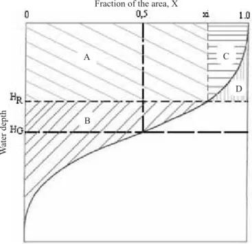
AND DISCUSSIONMathematical description of the deficit coefficient Figure 2 shows the graph of the cumulative probability density function for the normal distribution model, with the areas A, B, C and D defined. The quantity of water stored in the root zone is represented by A + C; the percolated wa-ter is represented by B and the wawa-ter deficit in the soil is represented by D.
According to Mantovani et al. (1995), one of the terms of CUC can be represented by the ratio between the sum of the model of the deviations in relation to the applied water depth and the required water depth. When the water distri-bution profile by the sprinklers follows a normal
distribu-tion, 50% of the area receives a water depth equal to the mean collected water depth (Walker 1979). Figure 2 shows the graph of the cumulative probability density function for the normal distribution model, with the areas A, B, C and D defined The quantity of water stored in the root zone is represented by A + C; the percolated water is represented by B; and the water deficit in the soil is represented by D.
According to Mantovani et al. (1995), one of the terms of the CUC can be represented by the ratio between the sum of the model of the deviation in relation to the applied wa-ter depth and required wawa-ter depth. When the distribution profile of the water by the sprinklers follows a normal dis-tribution, 50% of the area received a water depth equal to the mean collected water depth (Walker, 1979). By Figure 2, we have:
Anyoji (1994) presented the results of the area integra-tions, defined in the cumulative probability density function graph for normal distribution:
(20) =
∑HR ETc
Fraction of the area, X
W
ater
depth
A
B
C
D
Figure 2. Graph of the cumulative probability density function for the normal distribution model, with the areas A, B, C and D
(23)
( )
[Hx]dx A B
xi
0
+ =
∫
(21)
( )
[ ] [ ( )]
G 0 . 1
5 . 0
G 5
. 0
0
G
H
dx x H H dx H x H
1 CUC
∫
∫
− + −− =
(22)
( ) ( )
G 1
5 . 0
0 . 1
5 . 0 G 5
. 0
0
5 . 0
0 G
H
dx x H dx H dx H dx x H
1 CUC
∫
∫
∫
−∫
+ −− =
(24)
( )
[ ] 2 i
2
e 2
xi 0
dx=A+ =B x
H + µ.x
α −
Substituting Eq. 24 in Eq. 25 we have:
The sum of the areas A + B + C is equal to the mean applied water depth m because:
hence
Substituting µ for HG in Eq. 24, 25 and 26, µ for HG (Walker, 1979) and the term
Substituting Eq. 30, 31 and 32 in Eq. 21, we have:
In Figure 2, the water deficit in the soil corresponds to area D and can be defined as:
substituting Eq. 32 in Eq. 38 we have:
Isolating the term AD (fraction of the area where the wa-ter depth required by the crop was not applied) of equation proposed by Walker (1979), we have
Substituting ∆ = (HG – HR)/HG (Walker, 1979) in Eq. 45, we have:
and
Considering the water distribution pattern by the sprin-kler as a normal model, the Christiansen uniformity coeffi-cient (CUC) relates with the variation coefficoeffi-cient, by the fol-lowing ratio (Bernardo et al., 2006; Warrick & Gardner, 1983):
Substituting Eq. 49 in Eq. 47, we have (25) ( ) [ ] ∫ 1 0
dx=A+ + = µB C x
H
(26)
( )
[ ]
2
2
e
2
i
x
1
.
C
1 xi dx x Hα
−
π
σ
−
−
µ
=
⎜⎝⎛ ⎟⎠⎞ = ∫ (27) ( )[ ]
−
α
+
µ
π
σ
=
∫2
2
e
2
1 0 dx x H (28) ∞ → ∞ = α π σ ∞ → α α − π σ ∞ →α 0,as e
2 2 e 1 2 lim ou 2 2 e 2 lim (29) ( )
[ ]
=
µ
∫ 1 0 dx x H (32) ( )
[ ] G(1 xi) I
1
xi
H dx x
H = − −
∫
(30) 2 e 2 − πσ [ ( )]
i x . G xi 0 H I dx x
H = +
∫
por I, tem-se:
(31)
( )
[ ] G
1 0 H dx x H = ∫ (36) G H I 2 1 CUC= −
(35) G G G G G H I H 5 . 0 H 5 . 0 H 5 . 0 H 5 . 0 I 1
CUC= − + − + − +
(34) ( ) ( ) ( ) ([ ) ] G G G G G H I H 5 . 0 1 H 5 . 0 H 5 . 0 H 5 . 0 I 1
CUC= − + − + − − −
(33) ( ) ( ) ( ) [ ( ) ] G 0 . 1 5 . 0 i G 0 . 1 5 . 0 G 5 . 0 0 G 5 . 0 0 i G H I x 1 H H H x H I 1
CUC= − + − + − − −
(37)
( ) [H Hx]dx
H 1
i
x R
D= ∫ −
(38)
( )
∫ − ∫ = 1 i x 1 i x RD H dx H xdx
H
(41)
(1 x)(H H ) I
HD= − i R− G +
(39)
( )H [H (1 x) I]
H 1 G i
i x R
D= − − −
(40)
(1 x )H H (1 x ) I
HD= − i R− G − i +
(45) 301 . 0 1 cv 1.123 -cv 63 . 3 D
A ⎟⎟
⎠ ⎞ ⎜ ⎜ ⎝ ⎛ ∆ = (44) cv 1.123 -cv 63 . 3 301 . 0 D
A = ∆
(42) cv 301 . 0 D A 123 . 1 cv 63 . 3 − = ∆ (43) ∆
=3.63cv -cv 301 . 0 D A 123 . 1 (46) 301 . 0 1 cv 1.123 G H R H G H -cv 63 . 3 D A ⎟ ⎟ ⎟ ⎟ ⎟ ⎠ ⎞ ⎜ ⎜ ⎜ ⎜ ⎜ ⎝ ⎛ − = (47) 301 . 0 1 cv 1.123 G H R H 1 -cv 63 . 3 D A ⎟ ⎟ ⎟ ⎟ ⎟ ⎠ ⎞ ⎜ ⎜ ⎜ ⎜ ⎜ ⎝ ⎛ + = (48) cv 798 . 0 1 UC C (49) 798 . 0 CUC 1 cv= −
As AD = 100 − xi, we have:
where: Xi – fraction of the area where the water depth re-quired by the crop was applied, in percentage.
Dividing Eq. 53 by 30, xi is obtained between 0 and 1.
and
Substituting Eq. 52 in Eq. 41, we have
Isolating I in Eq. 36 we have:
Substituting Eq. 58 in Eq. 57 we have
The deficit coefficient was defined by Mantovani et al. (1995) as the ratio between the water deficit (HD) in the soil and the water depth required by the crop (HR). Substituting Eq. 59 in this ratio, the defined deficit coefficient is obtained when the water distribution profile by the sprinklers follows a normal cumulative probability density function.
Simplifying Eq. 60 we have
where:
CD– deficit coefficient, adimensional
HR– water depth required by the crop, in mm HG– gross water depth applied, in mm CUC – Christiansen uniformity coefficient, in %
Comparison of the results
The results of crop yield in the L1A, L1B, L2A, L2B, L3A and L3B treatments, obtained in the experiment carried out by Faccioli in 2000 and published in 2002, at the Coimbra Experimental Station, from August 10 to November 17, 2000, were compared with the results obtained using the produc-tion funcproduc-tion model by Mantovani et al. (1995), using the deficit coefficient, considering the water distribution profile by the sprinklers as uniform and normal.
According to the methodology presented, the maximum crop yield (Ymax) and the crop sensitivity coefficient to wa-ter deficit (β) considered were 3000 kg ha-1 and 1.15,
(51) ( ) ( ) 322 . 3 CUC 1 1.407 G H R H 1 -CUC 1 548 . 4 D A ⎟ ⎟ ⎟ ⎟ ⎟ ⎠ ⎞ ⎜ ⎜ ⎜ ⎜ ⎜ ⎝ ⎛ − + − = (52) ( ) ( ) 322 . 3 CUC 1 1.407 G H R H 1 -CUC 1 548 . 4 i x 100 ⎟ ⎟ ⎟ ⎟ ⎟ ⎠ ⎞ ⎜ ⎜ ⎜ ⎜ ⎜ ⎝ ⎛ − + − = − (53) ( ) ( ) 322 . 3 CUC 1 1.407 G H R H 1 -CUC 1 548 . 4 100 i x ⎟ ⎟ ⎟ ⎟ ⎟ ⎠ ⎞ ⎜ ⎜ ⎜ ⎜ ⎜ ⎝ ⎛ − + − − = (54) ( ) ( ) 100 322 . 3 CUC 1 1.407 G H R H 1 -CUC 1 548 . 4 100 i x ⎟ ⎟ ⎟ ⎟ ⎟ ⎠ ⎞ ⎜ ⎜ ⎜ ⎜ ⎜ ⎝ ⎛ − + − − = (55) ( ) ( ) 100 322 . 3 CUC 1 1.407 G H R H 1 -CUC 1 548 . 4 1 i x ⎟ ⎟ ⎟ ⎟ ⎟ ⎠ ⎞ ⎜ ⎜ ⎜ ⎜ ⎜ ⎝ ⎛ − + − − = (57) ( ) ( )
(H H ) I 100 CUC 1 1.407 H H 1 -CUC 1 548 . 4
H R G
322 . 3
G R
D − +
⎟⎟ ⎟ ⎟ ⎟ ⎟ ⎟ ⎟ ⎟ ⎠ ⎞ ⎜ ⎜ ⎜ ⎜ ⎜ ⎜ ⎜ ⎜ ⎜ ⎝ ⎛ ⎟⎟ ⎟ ⎟ ⎟ ⎠ ⎞ ⎜⎜ ⎜ ⎜ ⎜ ⎝ ⎛ − + − = (56) ( ) ( )
(H H ) I 100 CUC 1 1.407 H H 1 -CUC 1 548 . 4 1 1
H R G
322 . 3
G R
D − +
⎥ ⎥ ⎥ ⎥ ⎥ ⎥ ⎥ ⎥ ⎥ ⎦ ⎤ ⎢ ⎢ ⎢ ⎢ ⎢ ⎢ ⎢ ⎢ ⎢ ⎣ ⎡ ⎟⎟ ⎟ ⎟ ⎟ ⎟ ⎟ ⎟ ⎟ ⎠ ⎞ ⎜⎜ ⎜ ⎜ ⎜ ⎜ ⎜ ⎜ ⎜ ⎝ ⎛ ⎟⎟ ⎟ ⎟ ⎟ ⎠ ⎞ ⎜⎜ ⎜ ⎜ ⎜ ⎝ ⎛ − + − − − = (58) ( ) G H 2 CUC 1 I= −
(59)
( )
( )
( R G) ( ) G
322 . 3
G R
D .H
2 CUC 1 H H 100 CUC 1 1.407 H H 1 -CUC 1 548 . 4
H − + −
⎟⎟ ⎟ ⎟ ⎟ ⎟ ⎟ ⎟ ⎠ ⎞ ⎜⎜ ⎜ ⎜ ⎜ ⎜ ⎜ ⎜ ⎝ ⎛ ⎟⎟ ⎟ ⎟ ⎟ ⎠ ⎞ ⎜⎜ ⎜ ⎜ ⎜ ⎝ ⎛ − + − = (60) ( ) ( ) ( ) ( ) R G G R 322 . 3 G R D H H 2 CUC 1 H H 100 CUC 1 1.407 H H 1 -CUC 1 548 . 4 C − + − ⎟ ⎟⎟ ⎟ ⎟ ⎟ ⎟ ⎟ ⎟ ⎠ ⎞ ⎜ ⎜⎜ ⎜ ⎜ ⎜ ⎜ ⎜ ⎜ ⎝ ⎛ ⎟⎟ ⎟ ⎟ ⎟ ⎠ ⎞ ⎜⎜ ⎜ ⎜ ⎜ ⎝ ⎛ − + − = (61) ( ) ( ) ( ) R G R G 322 . 3 G R D H H 2 CUC 1 H H 1 100 CUC 1 1.407 H H 1 -CUC 1 548 . 4
C + −
respectively. The values of the maximum evotranspiration fraction replaced by other sources (p) and the uniform and normal deficit coefficients used in the production function model were the values presented previously.
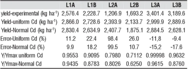
Table 1 shows the yields obtained in the experiment, the productivities simulated with the model, using the uniform and normal deficit coefficient, errors and simulated relative yield with the uniform and normal deficit coefficients for the L1A, L1B, L2A, L2B, L3A and L3B treatments.
Table 1 shows that for the L1A, L1B and L2B treatments, yield values simulated by the model, using the normal Cd, were closer to those obtained in the field than the simulated values, using the uniform Cd. Crop yield simulated by the model, using the uniform and normal Cd, were respectively for the L1A treatment 2,866.0 and 2,830.4 kg ha-1 for the L1A treatment, 2,728.6 and 2,634.9 kg ha-1 for the L1B treatment and 2,133.7 and 1,875.1 kg ha-1 for the L2B treatment. As reported previously, the normal Cd presented greater values than the uniform Cd, which meant that the yield values sim-ulated with a normal CD would always be lower than the val-ues simulated with the uniform Cd. As the maximum crop yield considered was 3,000 kg ha-1 and the L1A, L1B, L2A treatments presented an experimental crop yield of 2,576.4, 2,228.7 and 1,693.2 kg ha-1, respectively, the yield values sim-ulated with the uniform Cd were closer to the maximum yield and were more distant from the values obtained experimen-tally than the values simulated with the normal Cd. For the L2A treatment, this presented an experimental yield of 1,206.9 kg ha-1, the normal Cd generated by equation 15 was lower than the uniform Cd, therefore the yields simulated with the uniform Cd presented a better result. In this treatment, the yields simulated by the model, using the uniform and normal Cd, were 2,393.9 and 2,407.7 kg ha-1, respectively.
For the L3A and L3B treatments, crop yield values simu-lated by the model, using the uniform Cd, were closer to those obtained in the field than the values simulated with the normal CD. The productivities simulated by the model, using the uniform and normal Cd, were respectively, for treat-ment L3A 2,999.9 and 2,884.5 kg ha-1 for treatment L3A and 2,889.6 and 2,628.1 kg ha-1 for treatment L3B. In this case, the L3A and L3B treatments presented an experimental yield of 3,401.4 and 3,189.6 kg ha-1, respectively, and the yield values simulated with the uniform Cd, that were closest to
the maximum yield of 3,000 kg ha-1 were closer to the val-ues obtained experimentally than the valval-ues simulated with the normal Cd.
CONCLUSION
1. The relative yields values simulated by the model, us-ing the normal deficit coefficient, were always lower than the values simulated with the uniform deficit coefficient, for all the levels of uniformity and for all the values of the max-imum evotranspiration fraction of the crop replaced by oth-er sources (p.
2. Yield results simulated with the developed deficit co-efficient (normal distribution), were more fitted to the means in the field for the L1A, L1B and L2B treatments.
3. The treatments where the water depth applied was greater than the water depth required (L3A and L3B) crop yield simulated with the uniform deficit coefficient present-ed results better fittpresent-ed to the mean values in the field.
LITERATURE CITED
Anyoji, H.; Wu, I. P. Normal Distribution Water application for drip irrigation schedules. Transactions of the ASAE, v.37, p.159-164, 1994.
Bernardo, S.; Soares, A. A.; Mantovani, E. C. Manual de irrigação. 8.ed. Viçosa: UFV, 2006. 625p.
Cecon, P. R. Apostila de INF 662. Viçosa: UFV, 2001. 203p. Doorenbos, J.; Kassam, A. H. Yield response to water. Rome:
FAO, 1979. 193p. Irrigation and drainage Paper 33
Frizzone, J. A. Função de produção. In: Faria, M. A. de (org.). Manejo da irrigação. 1.ed. Lavras: SBEA, 1998. v.1, p.86-116. Faccioli, G. F. Modelagem da uniformidade da lâmina de irrigação na produtividade do feijoeiro. Viçosa: UFV, 2002. Tese Doutorado Gomide, F. L. S. Hidrologia básica. São Paulo: Edgard Blucher
Ltda. 1976. 278p
Hanks, R. J. Yield and water-use relationships: An overview. In: Taylor, H. M.; Jordan W. R.; Sinclair, T. R. (ed.). Limitations to efficient water use in crop production. Madison: American Society of Agronomy Crop Science Society of American Soil Science Society of American, 1983. p.393-411.
Karmeli, D. Estimating sprinkler distribution patterns using linear regression. Transactions of the ASAE, v.21, n.4, p.682-686, 1978. Mantovani, E. C.; Villalobos, F. J.; Orgaz, F.; Federes, E. Model-ling the effects sprinkler irrigation uniformity on crop yield. Agricultural Water Management, v.27. p.243-257. 1995. Stewart, J. I.; Hagan, R. M.; Pruitt, W. O.; Heanks, R. J.; Riley, J. P.;
Danielson, R. E.; Franklin, W. T.; Jackson, E. B. Optimizing crop production through control of water and salinity levels in the soil. Publ, PRWW 15 1 -1, Logan: Utah State University. 1977. 191p. Walker, W. Explicit splinker irrigation uniformity: efficiency model. Journal Irrigation and Drainage, ASCE, n.IR2, p.129-136, 1979.
Warrick, A. W.; Gardner, W. R. Crop yield affected by spatial vari-ations of soil and irrigvari-ations. Water Resource Research, v.19, n.1, p.181-186, 1983.
A 1
L L1B L2A L2B L3A L3B
a h g k ( l a t n e m ir e p x e -d l e i
y -1)2,576.4 2,228.7 1,206.9 1,693.2 3,401.4 3,189.6
a h g k ( d C m r o fi n u -d l e i
Y -1) 2,866.0 2,728.6 2,393.9 2,133.7 2,999.9 2,889.6
a h g k ( d C l a m r o N -d l e i
Y -1) 2,830.4 2,634.9 2,407.7 1,875.1 2,884.5 2,628.1
) % ( d C m r o fi n U -r o r r
E 11.2 22.4 98.4 26.0 -11,8 -9.4
) % ( d C l a m r o N -r o r r
E 9.9 18.2 99.5 10.7 -15,2 -17.6
d C m r o fi n u x a m Y /
Y 0.9553 0.9095 0.7980 0.7112 0.99998 0.9632
d C l a m r o N -x a m Y /
Y 0.9435 0.8783 0.8026 0.6250 0.9615 0.8760