Assessing the hardness of SVP algorithms in the presence of CPUs and GPUs

(1)

Universidade do Minho

Escola de Engenharia

Fábio José Gonçalves Correia

Assessing the Hardness of SVP Algorithms

on Multi-core CPUs

(2)

Universidade do Minho

Dissertação de Mestrado

Escola de Engenharia

Departamento de Informática

Fábio José Gonçalves Correia

Assessing the Hardness of SVP Algorithms

on Multi-core CPUs

Mestrado em Engenharia Informática

Trabalho realizado sob orientação de

Professor Alberto José Proença

Artur Miguel Matos Mariano

(3)

(4)

Acknowledgments

Ao meu orientador, Alberto Proença, quer pela disponibilidade total, quer pelo rigor exigido, assim como pelo apoio na escrita da dissertação. Ao meu co-orientador Artur Mariano, que sempre se mostrou disponível para discutir problemas relacionados com a tese e por me ter aberto a oportunidade de efectuar um estágio no âmbito da minha dissertação de mestrado na Alemanha.

Ao programa Erasmus Placements, que me possibilitou a experiência de estudar num país estrangeiro, a Alemanha, ajudando-me a evoluir tanto a nível pessoal, com muitas novas amizades, como a nível profissional, permitindo trabalhar num ambiente bastante diferente do que conhecia em Portugal.

I would like to thank the Institute for Scientific Computing for receiving me in Darmstadt. I would also like to thank Florian Göpfert, Özgür Dagdelen, Damien Stehlé and Erik Agrell for very useful discussions on lattices. A special thanks to Thomas Arneich for all the hours spent in discussions, which also lead to new ideas.

A todos os meus amigos de LEI que me suportaram durante o meu percurso académico e que me possibilitaram os melhores anos da minha vida, em especial ao Cristiano Sousa pelas várias discussões muito úteis durante o último ano.

Um agradecimento especial à minha família, pais e irmão, por todo o apoio que deram e que me ajudaram a chegar onde cheguei.

(5)

(6)

Abstract

Lattice-based cryptography has been a hot topic in the past decade, since it is believed that lattice-based cryptosystems are immune against attacks operated by quantum computers. The security of this type of cryptography is based on the hardness of algorithms that solve lattice-based problems, namely the Shortest Vector Problem (SVP). Therefore, it is important to assess the performance of such algorithms on High Performance Computing (HPC) systems.

This dissertation compares a wide range of algorithms that solve the SVP, the SVP-solvers, namely, the Voronoi cell-based algorithm and two enumeration-based solvers, SE++ and ENUM. We show that different techniques and optimizations used to significantly improve the performance of ENUM can also be applied to other enumeration algorithms, namely the extreme pruning technique and the optimization that avoids symmetric branches of the enumeration tree.

We present the first practical results of the Voronoi cell-based algorithm and compare its performance to the mentioned enumeration algorithms. The Voronoi cell-based algorithm performed considerably worse, although it displays potential for parallelization.

The optimization that avoids the computation of symmetric branches improved the performance of SE++ by almost 50%, thus outperforming ENUM by a factor of 3%, on the average. Parallel versions of the enumeration algorithms were implemented on a shared memory system based on a dual (8+8)-core device, which, in some instances, scale super-linearly for up to 8 threads and linearly for 16 threads. The parallel versions of the enumeration with extreme pruning algorithms were parallelized with MPI and achieved speedups of up to 12.96x with 16 processes with ENUM on a lattice in dimension 74.

We show that an efficient parallel implementation of ENUM can be integrated into BKZ, a lattice basis reduction algorithm, to parallelize it efficiently, since for high block-sizes almost all of the execution time of BKZ is spent on ENUM. This implementation of BKZ achieves speedups of up to 13.72x for a lattice in dimension 60, reduced with block-size 50. We also compared the quality of the output bases to other BKZ implementations, namely AC_BKZ, an implementation developed in colaboration with Thomas Arnreich, and G_BKZ_FP, an implementation publicly available in the NTL library. Our implementation showed to compute the bases with better quality, in the general case.

Finally, a novel parallel approach for the enumeration with extreme pruning is proposed. This approach promises to significantly improve the performance of the enumeration with extreme pruning, since much higher number of cores can be used to achieve higher speedups.

(7)

(8)

Resumo

A criptografia baseada em retículos tem vindo a tornar-se um tópico central ao longo da última década, dado que se acredita que criptosistemas baseados em retículos sejam resistentes a ataques infligidos com computadores quânticos. A segurança destes criptosistemas é medida pela eficácia dos algoritmos que resolvem problemas centrais em retículos, como o problema do vector mais curto. Por isso, é importante avaliar o desempenho destes algoritmos em arquitecturas computacionais de alto rendimento.

Esta dissertação compara uma grande variedade de algoritmos que resolvem o problema do vector mais curto, nomeadamente o algoritmo baseado em células de Voronoi e dois algoritmos de enumeração, o SE++ e o ENUM. Além disso, mostramos que é possível aplicar várias técnicas e optimizações do ENUM a outros algoritmos de enumeração, nomeadamente a técnica de poda extrema e a optimização que evita a computação de ramos simétricos da árvore de enumeração.

Foram ainda apresentados os primeiros resultados práticos do algoritmo de células de Voronoi, cujo desempenho foi comparado ao desempenho dos algoritmos de enumeração mencionados. O algoritmo baseado em células de Voronoi, apesar do apresentar potencial de paralelização, apresenta um desem-penho bastante pior que as restantes implementações.

A optimização que evita a computação de ramos simétricos acelera o SE++ em quase 50%, o que lhe permite ultrapassar o ENUM em termos de desempenho por um factor de 3%, no caso médio. Além disso, foram implementadas versões paralelas do algoritmos de enumeração, quer num sistema de memória partilhada baseado num dispositivo com 8+8 núcleos computacionais, para as variantes sem poda ex-trema, quer em memória distribuída, para as variantes com poda extrema. Os resultados mostram que as implementações em memória partilhada atingem, em certos casos, acelerações super-lineares até 8threads e lineares para 16 threads. As implementações em memória distribuída, por seu turno, são aceleradas em cerca de 13 vezes para 16 processos.

Também é mostrado que é possível integrar uma versão paralela eficiente do algoritmo ENUM no BKZ, um algoritmo de redução da base de um retículo, como forma de o paralelizar eficientemente, dado que a grande maioria do tempo de execução é gasto em chamadas ao ENUM para tamanhos de bloco grandes. Esta implementação alcança acelerações até 13.72 vezes para o retículo na dimensão 60, reduzido com um tamanho de bloco 50. A qualidade das bases dos retículos, computados por esta implementação, foi comparada a outros implementações do BKZ, nomeadamente o AC_BKZ, uma implementação desen-volvida em conjunto com Thomas Arnreich, e o G_BKZ_FP, uma implementação acessível publicamente na biblioteca NTL. A nossa implementação apresentou computar bases com uma qualidade superior às restantes, no caso geral.

(9)

algoritmos de enumeração com poda extrema significativamente, dado que poderá tirar partido de um maior número de núcleos computacionais.

(10)

List of Figures

2.1 Example of an heterogeneous platform. . . 6

2.2 Diagram of the Kepler architecture (from NVidia documentation). . . 8

3.1 Representation of the hipersphere in dimension i, which is divided into (i−1)-dimensional layers. . . 17

3.2 Workflow of the enumeration with extreme pruning. . . 21

4.1 Comparison of SE++ with the optimized version of the algorithm. . . 24

4.2 Representation of the symmetric subtrees whose computation can be avoided. . . 25

4.3 Execution time BKZ call, the extreme pruned enumeration call and the total execution time of our parallel implementation of both algorithms with extreme pruning running with 32 (+1) processes for a lattice in dimension 80. . . 27

4.4 Performance of different SVP-solver running in sequential. . . 28

4.5 Execution time of the sequential versions of three BKZ implementations for lattices in dimensions 60, 70 and 80, reduced with block-sizes 30, 35 and 40. . . 31

4.6 Map of the parallel enumeration workflow on a tree, partitioned into tasks, according to the parameters. In this example the parameters were set as MAX_BREADTH = 3 and MAX_DEPTH = n_{− log}₂(4T hreads). . . . 32

4.7 Workflow of the parallel enumeration with extreme pruning. . . 34

4.8 Performance of our improved SE++ implementation with 16 threads solving the CVP on random lattices in dimensions 52, 54 and 56, in (a), and number of tasks created for 4, 8, and 16 threads for a lattice in dimension 56, in (b). BKZ-reduced bases with block-size 20. . . 35

4.9 Performance of the SE++, ENUM and improved SE++ parallel implementations on a random lattice in dimensions 62. BKZ-reduced bases with block-size 20. . . 36

4.10 Performance of both parallel versions of BKZ for block-sizes 40, 45 and 50 for a lattice in dimension 60. . . 39

4.11 Performance of both parallel versions of BKZ for block-sizes 40, 45 and 50 for a lattice in dimension 70. . . 39

(13)

(14)

List of Tables

4.1 Specification of the CPU that was used for the tests. . . 23

4.2 Quality results for the lattice in dimension 60, reduced with block-sizes 30, 35 and 40, for the different criteria. . . 30

4.3 Quality results for the lattices in dimensions 70 and 80, reduced with block-size 40, for the different criteria. . . 30

4.4 Speedup (S) and efficiency (E) of SE++ for 6 lattices, whose bases were reduced with BKZ with block-size 20. . . 36

4.5 Speedup (S) and efficiency (E) of ENUM for 6 lattices, whose bases were reduced with BKZ with block-size 20. . . 37

4.6 Speedup (S) and efficiency (E) of the improved SE++ for 6 lattices, whose bases were reduced with BKZ with block-size 20. . . 37

4.7 Speedup (S) and Efficiency (E) of the parallel SE++ algorithm with extreme pruning for 6 lattices, whose bases were reduced with BKZ with block-size 20. . . 38

4.8 Speedup (S) and Efficiency (E) of the parallel ENUM algorithm with extreme pruning for 6 lattices, whose bases were reduced with BKZ with block-size 20. . . 38

4.9 Speedup (S) and Efficiency (E) of both parallel BKZ implementations for a lattice in di-mension 60 for block-sizes 40, 45 and 50. . . 40

4.10 Speedup (S) and Efficiency (E) of both parallel BKZ implementations for a lattice in di-mension 70 for block-sizes 40, 45 and 50. . . 40

(15)

(16)

Chapter 1 Introduction

Lattices are discrete and infinite subgroups of the m-dimensional Euclidean space Rm_{. A lattice} L is

generated by all linear combinations of a basis B, a set of linearly independent vectors b1,...,bn inRm,

and is denoted by:

L(B) = {x ∈ Rm _{: x =} n

∑

i=1

cibi, c∈ Zn} (1.1)

where n is thedimensionof the lattice.

Vectors and matrices are represented in this dissertation in bold face, vectors in lower-case and matrices in upper-case, as in vector v and matrix M. The auxiliary functions used by the algorithms are written as in

function(). The dot product of two vectors v and p is denoted by⟨v,p⟩. The transpose of a matrix is given

by MT_. _{⌈a⌋ rounds}_a_{to the nearest integer number. The absolute value of a is given by}_|a|.

The Euclidean norm of a vector v_{∈ R}n_{, denoted by}_||v||

2or simply||v||, is the distance spanned from

the origin of the lattice to the point given by the vector v, i.e. _{||v|| =} √∑n i=1v

2

i, where vi is the ith

coordinate of v. The norm of the shortest vector of the lattice is given by λ1(L(B)).

Lattices and basis reduction algorithms are used to solve relevant problems in mathematics and com-puter science. A reduced basis is a basis where the vectors are short and nearly orthogonal. In mathemat-ics, an example is the study of the geometry of numbers (Cassels,1997). In computer science, lattices has played a key role in the theory of integer programming (Lenstra,1983;Kannan,1987), in factoring poly-nomials over the rationals (Lenstra et al.,1982), in solving low density subset-sum problems (Coster et al.,

1992), in checking the solvability by radicals (Landau and Miller,1985) and in solving many cryptanalytic problems (Odlyzko,1990;Bellare et al.,1997;Joux and Stern,1998;Nguyen and Stern,2001).

Lattice-based cryptography has been a hot topic in the past decade, since lattice-based cryptosystems are believed to be resistant against attacks operated with quantum computers. Cryptosystems based on lattices are said to be secure when specific lattice problems can not be solved in a timely manner.

Well known mathematical problems based on lattices are the shortest vector problem (SVP) and the closest vector problem (CVP). The SVP aims to find the shortest non-zero vector of the lattice, i.e., to find x∈ Zn_{\0 minimizing ∥B · x∥ in the Euclidean norm. The CVP aims to find the closest lattice vector to a}

given target vector t _{∈ R}m_{, i.e., to find x} _{∈ Z}n_{that minimizes} _{∥B · x − t∥. Both have been proved to}

(17)

CHAPTER 1. INTRODUCTION

studied to be exactly solved and also to efficiently find approximate solutions. Algorithms that solve the SVP are known as SVP-solvers, while algorithms that solve the CVP are known as CVP-solvers.

1.1 Motivation & Goals

Lattice-based cryptography has gained a renewed interest in the past decade, since it is believed that cryptosystems based on lattices can be more resistant to attacks, even when operated with quantum computers. Lattice-based cryptosystems are secure when specific lattice problems can not be solved in a timely manner. This dissertation focuses on two classes of algorithms that solve the SVP, one of the problems in question.

In the last decade, SVP-solvers have been thoroughly studied. New algorithms were proposed (e.g.,

(Micciancio and Voulgaris, 2009; Gama et al., 2010)) and some existing algorithms were optimized to

achieve a higher performance (e.g., (Blömer and Naewe,2009;Fitzpatrick et al.,2014)). Recently, some parallel implementations were also proposed (Dagdelen and Schneider,2010;Mariano et al.,2014b).

Enumeration algorithms are currently the fastest in practice, mainly due to a specific technique, extreme pruning. This motivated the implementation of two enumeration algorithms and the application of the extreme pruning technique on them, followed by a performance assessment of the implementations of both algorithms, with and without extreme pruning. After this analysis, this dissertation also aimed to implement efficient parallel versions of the algorithms that would significantly speed them up.

Research in another algorithm, the Voronoi cell-based algorithm, has not been aimed as much as the others in the past. This algorithm seems to display potential for an efficient parallel implementation. This motivated us to implement this algorithm, showing the first practical results.

Finally, one of the most important components in every algorithm related to lattices is a lattice basis pre-processing, the lattice basis reduction mentioned earlier. Efficient lattice basis reduction algorithms could lead to stronger basis reductions, which could reduce the execution time of SVP-solvers considerably. Another goal of this work is to efficiently parallelize one of these lattice basis reduction algorithms, the BKZ, which is currently one of the most used in practice.

1.2 Contribution

The work developed during this dissertation lead to several scientific contributions in the field related to SVP-solvers. These include:

• Efficient implementations of several SVP-solvers and BKZ, from sequential to parallel versions, most of them not publicly available; List of algorithms:

– Sequential Voronoi cell-based algorithm.

– Enumeration, namely sequential and parallel SE++, ENUM, both with and without extreme pruning, and the improved SE++, a variant with an optimization that avoids the computation

(18)

1.3. OUTLINE

of symmetric branches of the enumeration tree.

– Lattice basis reduction, namely sequential and parallel BKZ implementations, which internally use the LLL algorithm and the Gram-Schmidt orthogonalization.

• A comparative performance evaluation of several SVP-solver implementations, both sequential and parallel.

• A basis quality assessment of BKZ implementations.

• Proposal of a novel parallel implementation that merges ENUM (with extreme pruning) with the parallel BKZ reduction, on distributed memory systems.

1.3 Outline

The rest of this dissertation is organized as follows. Chapter 2details the kind of computing platforms our implementations will target and their characteristics. Chapter 3presents the current approaches to reduce the lattice basis and the key algorithms to solve the SVP. Chapter 4discusses the performance results achieved with the implemented sequential and parallel versions of the algorithms. It also assesses the lattice basis quality, comparing our implementations with the ones available at the NTL1_{library. Chapter}

5concludes the dissertation with a critical analysis of the obtained results, leaving suggestions for future work on relevant topics that could not be fully covered on this dissertation.

(19)

(20)

Chapter 2 Target Platforms

Computer clusters are currently the most used systems for High Performance Computing (HPC). A cluster is built of a set of interconnected computing nodes, where each node may have one or more multi-core CPU devices and eventually a computing accelerator, for example, a GPU (Graphics Processing Unit) or a many-core CPU device, such as the Intel Many Integrated Cores (MIC) device. When a node or a computing system has attached an accelerator, we consider this system to be heterogeneous.

A program can be executed on a single node or on multiple nodes of a cluster. If the program is prepared to explore parallelism it will, therefore, distribute its work among the available resources to reduce its execution time. There are two major paradigms in parallel computing: shared memory and distributed memory.

On the shared memory paradigm, the processors work on different tasks of a program, each implemen-ted as a process or a thread. When tasks are implemenimplemen-ted as threads, a single copy of the data can reside in a global memory, shared among all threads.

In the distributed memory model, the work and associated data is distributed by multiple computing nodes. This is particularly useful for programs where a large data domain can be partitioned by several independent memory banks, allowing each node to compute only on part of the data, increasing the performance of the program.

Another paradigm that is becoming more used is a hybrid paradigm, which joins the advantages of shared memory with distributed memory. In this approach, each node has a smaller data block and the different cores of a node work on the same block.

2.1 The Architecture

The parallel implementations of the SVP algorithms in this dissertation work, aimed the heterogeneous nodes as the main target platform, where the CPU devices were Intel Xeon, based on the Sandy Bridge micro-architecture.

With the increasing demand on architectures that simultaneously compute massive amounts of data, 2 types of heterogeneous HPC systems have emerged: systems using GPUs as attached computing ac-celerators and systems using the Intel Xeon Phi (based on the Many Integrated Core architecture - MIC)

(21)

CHAPTER 2. TARGET PLATFORMS

as accelerators. Figure2.1shows an example of an heterogeneous platform, which uses multiple CPU devices and multiple accelerators to perform their computation.

Local Memory Hierarchy Core Core Core Core Local Memory Hierarchy Core Core Core Core CPU CPU Local Memory Hierarchy Accelerator Interface Local Memory Hierarchy Accelerator

Figure 2.1: Example of an heterogeneous platform.

2.2 Computing Accelerators

The MIC is a multiprocessor computer architecture developed by Intel. It is possible to use programming languages, models and tools from traditional Intel Xeon processors on this architecture. Implementations for Intel Xeon processors will also work on Intel Xeon Phi coprocessors. But to get high performance out of this device, further improvements and optimizations have to be done. Currently, MIC coprocessors provide up to 61 cores and hardware support for 4 threads per core. Knights Corner, the current Xeon Phi implementation, uses for each core an updated version the old Pentium P54C, which only supports in-order execution and SIMD instructions on 512 bit data (from the previous Intel Larrabee, not compatible with SVX-512). Although each core has 2 private cache levels, while usual Xeons have a large third level cache (L3), the data on all all L2 caches can be accessed by all cores as a L3 cache. On the other hand, Knight Landing, the next generation MIC-based architecture, use Airmont (14-nm Atom) core and supports 384 GB of DDR4 RAM and AVX-512F (AVX3.1) SIMD instructions.

However, other heterogeneous platforms use GPUs as accelerators. Their optimization in programs that execute the same instructions over multiple data and their high bandwidth allows them to reach higher performances than CPUs in many problems.

(22)

2.3. DEVELOPMENT AIDS FOR HETEROGENEOUS PLATFORMS

Early GPU devices were specifically designed for computer graphics, where images are rendered from geometric objects. The color of the pixels that constitute the image are computed in parallel and sent to the screen. When GPUs started to increase their complexity and performance, the interest in using them in scientific computing also increased. A GPU is accessed and controlled by the CPU, but to allow concurrent execution and memory transfer, they work asynchronously.

NVidia GPUs used in HPC have the following organization:

• several SIMD (Single Instruction Multiple Data) cores, where NVidia refers to these as Streaming Multiprocessors (SMs) and on the latest Kepler architectures NVidia changed into next-generation SMs or in short, SMXs (up to 16 SMXs).

• each SIMD core in Kepler has 192 Streaming Processors (SPs), also known as CUDA processors, basically, a single precision Floating Point (FP) unit and an Integer unit; previous Fermi generation had 32 SPs per SM.

• additional functional units at each SM/SMX, including double precision FP units and load/store units.

• each SIMD core in Kepler has 64K 32-bit registers, 48 KB read-only data cache and 64KB of configurable L1 cache and local memory.

• 1.5MB shared L2 cache in Kepler, doubles the L2 in Fermi.

• SMT (Simultaneous Multi-threading) support for up to 64 warps per SMX (in Kepler); warps are described below.

Figure2.2shows a diagram of the Kepler architecture. Current NVidia GPUs can be programmed using CUDA (Compute Unified Device Architecture). CUDA allows to do this by using a familiar language, like C or Fortran, just by adding specific directives for the execution on GPUs. CUDA uses a large number of threads organized into blocks to operate in a SPMD model. All blocks run the same program, where threads of the same block can communicate between them using a local memory shared among all threads of a block. Blocks are also split intowarps. Eachwarpconsists of 32 threads and all threads of the samewarp

execute the same instruction (following the SIMD model). At runtime, blocks are scheduled to SMs/SMXs. To abstract the programmer from these technical details and to aid in the development of efficient applications, specific frameworks for heterogeneous programming have been developed. This allows the programmer to focus more on algorithmic problems, instead of wasting time with details related to multi-platform implementations or data management.

2.3 Development Aids for Heterogeneous Platforms

Programming efficiently GPUs requires a great knowledge about the target architecture to get the maximum performance, for example memory and thread organization. So, the programmer has to take into account

(23)

CHAPTER 2. TARGET PLATFORMS

Figure 2.2: Diagram of the Kepler architecture (from NVidia documentation).

the way how data is organized in memory, thread scheduling,... There is also the risk of portability that when changing the system the performance might drop. To automate all this process of memory manage-ment, thread scheduling and portability, heterogeneous development frameworks have been created, e.g., StarPU (Augonnet et al.,2011) or GAMA(Barbosa,Sept. 2012). However, the main aim of heterogeneous development frameworks is to allow the simultaneous execution of a program on multi-core CPUs and GPUs.

StarPU, currently one of the most used heterogeneous frameworks, is a software tool that supports C extensions and aims to allow programmers to exploit the available resources, multi-core CPUs and GPUs, relieving them from the need to adapt their code to the target platforms. This framework is responsible to schedule tasks at runtime on CPU and/or GPU implementations and automatically manage data transfers on available CPUs and GPUs. This way, the programmer does not have to worry about scheduling issues and technical details associated with these data transfers.

Two of the most important data structures in StarPU are codelets and tasks. A codelet is a computational kernel that can be executed on distinct computational units, such as a multi-core CPU, a CUDA device or an OpenCL device. A task applies a codelet on a data set on the architecture where the codelet is implemented and controls how it is accessed (read and/or write). A task is an asynchronous operation and, therefore, submitting a task is also a non-blocking operation. A task can also define its priority as hint to the scheduler or a callback function, which is executed once the task is completed.

Tasks can also have data dependencies between them, which forces a sequential execution. A task might be identified by a unique number, called tag. Dependencies between tasks can be expressed by

(24)

2.3. DEVELOPMENT AIDS FOR HETEROGENEOUS PLATFORMS

callback functions, by submitting other tasks or by expressing dependencies between tags.

Since tasks are scheduled in runtime, data has to be transferred automatically between processing units relieving the programmer from explicit data transfers. To avoid unnecessary data transfers, StarPU allows to keep multiple copies of the same data on different processing units as long as it is not modified and to store data where it was lastly needed even if it was modified.

(25)

(26)

Chapter 3 The Shortest Vector Problem on Lattices

The shortest vector problem aims to find the shortest non-zero vector of the lattice, i.e., to find x∈ Zn_\0

that minimizes_{∥B · x∥ in the Euclidean norm. This problem has been extensively studied during the last} decades and three main families of SVP-solvers have emerged: sieving, enumeration and Voronoi cell-based algorithms. Sieving is a class of probabilistic and randomized algorithms that sieve a list of vectors, until a given stop criterion is met. Enumeration algorithms list all possible vectors within a given search radius and return the shortest among them. Voronoi cell-based algorithms compute the Voronoi relevant vectors and choose the shortest among them, which is also the shortest vector of the lattice.

The primary enumeration algorithm currently used is ENUM, which was proposed by Schnorr and Euch-ner (Schnorr and Euchner,1994) and improved by Gama et al. (Gama et al.,2010). Another enumeration algorithm, SE++, based on ENUM, was proposed by Agrell et al. (Agrell et al., 2002) and improved by Ghasemmehdi and Agrell (Ghasemmehdi and Agrell, 2009). Although SE++ was originally proposed to solve the CVP, it was presented in (Agrell et al.,2002) how to transform it into an SVP-solver. Currently, the fastest probabilistic approach to solve the SVP, in practice, is an heuristic based on enumeration algorithms, the enumeration with extreme pruning (Gama et al.,2010).

The performance of SVP-solvers depend strongly on the quality of the basis. The more reduced the basis is, i.e., the shorter and more orthogonal the basis vectors, the faster they find a solution for the SVP. Such bases can be computed by performing a lattice basis reduction. Lattice basis reduction and SVP-solvers have a strong relation, since lattice basis reduction algorithms compute an approximate version of the SVP and use SVP-solvers as part of their logic to improve the quality of the computed basis.

3.1 Lattice Basis Reduction

Lattice basis reduction is the process of transforming a basis B into another basis B’, whose vectors are reasonably short and nearly orthogonal. The quality of a basis depends on the shortness and orthogonality of the basis vectors. The shorter and more orthogonal the basis vectors, the better the quality of the basis, thus reducing the execution times of SVP- and CVP-solvers. The two most common lattice basis reduction algorithms in practice are the Lenstra-Lenstra-Lovász (LLL) and the Block Korkine-Zolotarev (BKZ).

(27)

CHAPTER 3. THE SHORTEST VECTOR PROBLEM ON LATTICES

polynomial time, it only generates a basis of moderate quality. A basis is considered LLL-reduced if it is size-reduced and if_∥b∗_i_{∥ ≥ ∥b}∗_i₋₁_{∥/2, ∀i ∈ {2..n}. A size-reduced basis is a basis where µ}i,j ≤ 1/2

for any i > j.

Another lattice basis reduction algorithm is the Hermite-Korkine-Zolotarev (HKZ). The basis vectors com-puted by this algorithm are more orthogonal, but it is also more expensive to compute them (Hanrot and

Stehlé,2008). A basis is HKZ-reduced if it is size-reduced, if b2, ..., bnare also HKZ-reduced when b1 is

orthogonally projected, and if∥b1∥ = λ1(L(B)).

The BKZ algorithm, proposed by Schnorr and Euchner (Schnorr and Euchner, 1994), combines the efficiency of the LLL with the quality of HKZ. This algorithm uses a sliding window on the basis and performs successively ENUM calls over the window as the basis is being traversed. If a shorter vector is found, it is added to the basis, which generates a dependency. This dependency is removed by an LLL reduction. The SVP is performed by the ENUM enumeration algorithm.

In 2011, another lattice basis reduction algorithm, BKZ 2.0, was proposed by Chen and Nguyen (Chen

and Nguyen,2011). This algorithm is an optimized version of the BKZ reduction algorithm that significantly

reduces the execution time of BKZ by applying: (i) an early-abort, which stops the algorithm after a certain number of iterations instead of only stopping when it is no longer possible to get a better basis; (ii) a stronger lattice basis reduction on each block, by using BKZ instead of LLL; (iii) a maximum search radius on the ENUM to improve its performance; (iv) sound pruning, where specific bounding functions are used to significantly decrease the execution time of ENUM. Despite of being the best lattice basis reduction algorithm at the moment, there are some crucial details for its implementation that were omitted on the original paper, which are still not clear (e.g., the bounding functions used for the sound pruning).

Recently, Liu et al. proposed a new variant of the BKZ algorithm and parallelized it on distributed memory systems, using MPI (Liu et al.,2014). From here on, we will call one traversal of the sliding window over the basis, from the beginning to the end, one round. This implementation uses n processes to compute the ENUM calls of one round in parallel. Instead of performing an LLL-reduction after each ENUM call, it inserts the shorter vectors found by ENUM into the basis at their respective positions and reduces this new set of vectors at the end.

3.1.1 LLL Reduction

The LLL algorithm is fed with the coefficients and square norms of the Gram-Schmidt matrix. It reduces the basis iteratively. The index k indicates that, at any given moment, the basis vectors (b1, ..., bk−1) are

LLL-reduced. The value of k can be either incremented or decremented at each loop iteration and stops when it reaches n + 1, when the entire basis (b1, ..., bn) is guaranteed to be LLL-reduced.

On each iteration, the algorithm computes a size-reduction of the vector bk, as in Algorithm1. Afterwards,

the Lovász condition is checked. If the Lovász condition holds true, nothing happens and the algorithm proceeds with the size-reduction of the next vector. Otherwise, the vector bkis swapped with its predecessor

bk−1.

Schnorr and Euchner proposed a variant of the LLL algorithm that is called LLL with deep insertions

(28)

3.1. LATTICE BASIS REDUCTION

Algorithm 1: The size-reduction algorithm, as in Figure 2, presented in (Nguyen and Stehlé,2006). Input: A basis (b1, ..., bn), its Gram-Schmidt orthogonalization and an index k.

Output: The basis where bkis size-reduced and the updated Gram-Schmidt orthogonalization.

1 fori=k-1down to1do 2 b_k= b_k− ⌈µ_k,i⌋b_i; 3 forj = 1toido

4 µ_k,j = µ_k,j− ⌈µ_k,i⌋µ_i,j;

5 Update the Gram-Schmidt orthogonalization ;

(Schnorr and Euchner, 1994). This algorithm replaces the swapping step by a “deep insertion”, which

improves the quality of the output basis significantly. When performing a deep insertion, the algorithm, instead of swapping the vector bk with its predecessor, computes the index where to insert the vector bk

by consecutively performing Lovász tests with the preceding vectors, until it holds true. The vector bk is

then inserted right before the last vector where the Lovász condition is violated. The pseudo-code of the algorithm is presented in Algorithm2.

Algorithm 2: The LLL algorithm, as in Figure 1, presented in (Nguyen and Stehlé,2006). Input: A basis (b1, ..., bn) and δ∈ (1/4, 1).

Output: An LLL-reduced basis with factor (δ, 1/2).

1 Compute the Gram-Schmidt orthogonalization, i.e., all µ_i,j’s and c_i’s ; 2 k = 2;

3 while k≤ n do

4 Size-reduce b_kusing Algorithm1; 5 k’ = k ;

6 while k ≥ 2 and δc_k₋₁ > c_k′+∑_i=kk′−1₋₁µ2_k′_,icido

7 k = k− 1 ; 8 fori = 1tok - 1do 9 µ_k,i= µ_k′_,i;

10 Insert b_k′ right before b_k ;

11 k = k + 1 ; 12 return (b₁, ..., b_n) ;

LLL with Floating Point Arithmetic

The original LLL reduction algorithm was created to reduce a lattice using rational arithmetic. Floating-point arithmetic can speed up the lattice reduction process, but it can also introduce floating-Floating-point errors. These errors can not only cause the algorithm to produce incorrect results, but they also might prevent the algorithm to terminate.

The first theoretically provable floating-point variant of the LLL was proposed by Schnorr (Schnorr,1988). A more efficient provable variant, L2_{, was proposed by Nguyen and Stehlé (}_{Nguyen and Stehlé}_, ₂₀₀₅_).

(29)

success probability. One important heuristic algorithm was proposed by Schnorr and Euchner (Schnorr

and Euchner,1994). It has been the inspiration for more recent algorithms, like the L2_{mentioned above.}

3.1.2 BKZ Reduction

The BKZ reduction is a compromise between the LLL and the HKZ reduction and receives the block-size

β as parameter. For β = 2, the algorithm outputs an LLL-reduced basis.When β = n, where n is the

dimension of the lattice, the algorithm outputs an HKZ-reduced basis. For higher values of β, the basis is more reduced but it also takes more time to perform the reduction. The pseudo-code of the algorithm is presented in Algorithm3.

Algorithm 3: The BKZ algorithm, as in Algorithm 1, presented in (Chen and Nguyen,2011). Input: A basis (b1, ..., bn), its Gram-Schmidt orthogonalization, i.e., µ and ci, a block-size

β ∈ 2, ..., n and δ ∈ (1/4, 1).

Output: A BKZ β-reduced basis.

1 z = 0 ; 2 j = 0 ; 3 LLL((b₁, ..., b_n), δ) ; 4 while z < n− 1 do 5 j = (j mod(n− 1)) + 1 ; 6 k = min(j + β− 1, n) ; 7 h =min(k + 1, n) ; 8 v =ENUM(µ_[j,k],c_j,k; 9 if v̸= (1, 0, ..., 0) then 10 z = 0 ; 11 LLL((b₁, ...,∑k_i=jv_ib_i, b_j, ..., b_h), δ) ; 12 else 13 z = z + 1; 14 LLL((b₁, ..., b_h), δ) ; 15 return (b₁, ..., b_n) ;

The algorithm starts by LLL-reducing the basis. Then it uses a sliding window, which contains at most

β vectors and traverses the basis from the beginning until the end. Each window ranges from j to k =

min(j + β − 1, n), where j is the index of the first basis vector of the window and k the index of the last basis vector of the window. For each block B[j,k], the enumeration algorithm ENUM is called.

Whenever a shorter vector bnew _{is found, it is inserted into the basis on the position right before the}

beginning of the block, between the vectors bj−1 and bj. This insertion generates a linear dependency

between the basis vectors. The linear dependency is removed by calling the LLL algorithm on the set of vectors (b1, ..., bj−1, bnew, bj, ..., bh), where h =min(k + 1, n). If a better vector is not found, the LLL

reduction is computed over B[1,h]to make sure that the next ENUM call is performed over an LLL-reduced

window.

When the last window is computed, i.e., when j = n_{− 1 and k = n, it jumps back to the beginning}

(30)

3.2. SIEVING ALGORITHMS

of the basis by setting j back to 1. This process is repeated until the enumeration call does not output shorter vectors n _{− 1 times consecutively, which means that the basis did not change for all indices} 1≤ j ≤ n − 1.

3.2 Sieving Algorithms

A key issue in sieving algorithms is vector reduction, which consists in subtracting one vector by another, in order to make it short. The first sieving algorithm to solve the shortest vector problem, was proposed in 2001 by Ajtai, Kumar and Sivakumar, also known as AKS (Ajtai et al.,2001). This algorithm takes a large list of vectors and reduces them by one another, until two vectors are obtained such that their difference is the shortest non-zero vector of the lattice.

The AKS was simplified by Nguyen and Vidick (Nguyen and Vidick, 2008), who also introduced an heuristic variant of the algorithm with much smaller asymptotic complexity. Further improvements on AKS were proposed in 2009 (Blömer and Naewe,2009) and on Nguyen and Vidick’s heuristc in 2011 (Wang et al.,2011).

Other researchers proposed an efficient variant of the AKS, ListSieve, and its heuristic counterpart, GaussSieve (Micciancio and Voulgaris,2009). These algorithms built a list of vectors instead of starting with a large lists. Then, the vectors are used to reduce the vectors that are incrementally sampled and added to the list. While ListSieve only reduce the sampled vectors against the elements in the list, GaussSieve, on the other hand, also reduces the list with the sampled vectors. Recently, a comprehensive comparison between ListSieve and GaussSieve has been perfomed (Mariano et al.,2014a) and further improvements on GaussSieve were also proposed (Fitzpatrick et al.,2014).

In 2011, Milde and Schneider (Milde and Schneider, 2011) proposed a parallel implementation of GaussSieve. However, the implementation changes the workflow of the algorithm and requires more iterations to converge as more threads are used, therefore, limiting its scalability. In 2013, a new parallel approach was presented that scales much better than Milde’s and Schneider’s, since it does not increase the time for the algorithm to converge at such a high pace as the first implementation (Ishiguro et al.,

2013). However, this version extends the computation done by the original algorithm. Currently, the most efficient and scalable parallel implementation of GaussSieve consists in replacing the list of vectors by a lock-free list, atomically making any modification of this list (Mariano et al.,2014b).

3.3 Enumeration Algorithms

P. van Emde Boas showed, in 1981, that the general closest vector problem as a function of the dimension

n is NP-hard (Boas,1981). The breakthrough papers in the SVP and the CVP date back to 1981, when Pohst presented an approach that examines lattice vectors that lie inside a hypersphere (Pohst, 1981), and to 1983, when Kannan showed a different approach using a rectangular parallelepiped (Kannan,

(31)

and Pohst,1985), and by Kannan (following Helfrich’s work (Helfrich,1985)), in 1987 (Kannan,1987). In

1994, Schnorr and Euchner proposed a significant improvement of Pohst’s method (Schnorr and Euchner,

1994), that was later on found to be substantially faster than Pohst’s and Kannan’s approaches (Agrell

et al., 2002). The improvement proposed by Schnorr and Euchner was influenced by the Nearest Plane

algorithm by Babai, a polynomial-time method to find vectors that are close to a given target vector (Babai,

1986). Recently, Ghasemmehdi and Agrell showed that there are some redundant operations in the algorithm that can be eliminated, accelerating it substantially (Ghasemmehdi and Agrell,2009).

In 2010, a new technique to solve the SVP, the enumeration with extreme pruning, which reduces the probability of finding the shortest vector, but also reduces the execution time, and by a much higher pace

(Gama et al.,2010). This technique was applied to ENUM, the enumeration algorithm proposed by Schnorr

and Euchner (Schnorr and Euchner,1994).

Recently, Micciancio and Walter presented a new enumeration algorithm that outperforms other enu-meration algorithms that do not use the extreme pruning technique by changing the basis pre-processing

(Micciancio and Walter,2014). However, it is still not known yet if the extreme pruning technique can be

applied to this algorithm.

There is also work published on the parallelization of enumeration algorithms. On multi-core CPUs, Dagdelen and Schneider proposed an approach that distributes work among threads using a list, where only one thread may add work if there is any idle thread was proposed in (Dagdelen and Schneider,2010). For GPUs, an implementation, where a CPU is used to create tasks that the GPU will compute when they get assigned, was proposed in 2010 (Hermans et al.,2010). After a given number of iterations the algorithm stops and might keep computing the same task or start computing a different, depending on whether the previous task did already finish or not. Recently, (Kuo et al.,2011) proposed an approach, based on (Hermans et al.,2010), for the enumeration with extreme pruning was proposed. This approach performs multiple calls to an extreme pruned enumeration algoritthm, running simultaneously on CPU and GPU, and uses a map-reduce to join the vectors at the end and to select the shortest.

3.3.1 SE++

The SE++ was initially proposed as a CVP-solver, although a variant to solve the SVP was also proposed in

(Agrell et al.,2002). Ghasemmehdi and Agrell proposed an improvement for the CVP-solver that consists

in avoiding redundant operations.

The SE++ algorithm can be separated in two different phases: the basis pre-processing and the sphere decoding. In the pre-processing phase, the matrix that contains the basis vectors, denoted by B, is reduced (e.g., with the BKZ or LLL algorithms). The resultant matrix D, is transformed into a lower-triangular matrix, which we refer to as G, with either the QR decomposition or the Cholesky decomposition (see (Agrell et al.,

2002) for further details). This transformation can be seen as a change of the coordinate system. The decomposition of D also generates an orthonormal matrix Q. Finally, the sphere decoding is fed with the dimension of the lattice n and the inverse of G, i.e., H = G−1, which is itself a lower triangular matrix.

There are two different ways of thinking about the sphere decoding process. Mathematically, it is the

(32)

3.3. ENUMERATION ALGORITHMS O √C 1 / Hi,i _ ui yi ei-1

Figure 3.1: Representation of the hipersphere in dimension i, which is divided into (i_{− 1)-dimensional layers.}

cess of enumerating lattice points inside a hypersphere, which is presented in Figure3.1. Algorithmically, this can also be described as a traversal of a tree.

As mentioned before, the sphere decoding consists in finding the shortest vector of the lattice inside a hypersphere, i.e., the closest vector to the origin of the lattice, which also denotes the center of the hypersphere. √C is the norm of the best vector found so far, denoted by û. √C also represents the

radius of the hypersphere. The implementation of the sphere decoding process is shown in Algorithm4, wheresign(a) returns -1 if a ≤ 0 and 1 otherwise, andround(a) rounds a to the nearest integer number. Lattices can be divided into lower-dimensional layers, where the dimension of the layer that is currently being examined, is, from here on, denoted by i. Each i-dimensional layer can be divided into (i− 1)-dimensional parallel layers, where 1/Hi,irepresents the distance between the layers.

The algorithm iterates over all the layers. It starts in the n-dimensional layer and stops when this layer is reached again. We will refer to the process of visiting a lower-dimensional layer (decrementing i) as

moving downand the process of visiting a higher-dimensional layer (incrementing i) asmoving up. For each dimension, the coefficients ei of the projection onto the basis vectors, where ei = (Ei,1, Ei,2

, . . . , Ei,n)∈ Rn, and the orthogonal displacement yi from the projected vector to the current layer are

calculated. The (i_{− 1)-dimensional layer that is being examined is determined by u}ias a coefficient. The

(i− 1) parallel layers are visited in a zigzag pattern, based on the Schnorr-Euchner refinement (Schnorr

and Euchner,1994). ∆icontains the step that has to be taken to visit the next (i− 1)-dimensional layer

and is used to update ui. The squared distance from the origin of the lattice to the layer that is being

analyzed is denoted by disti. If disti < C the algorithm willmove down, otherwise it willmove upagain.

When the zero-dimensional layer is reached, the coefficient vector u, is stored in û and the value of C is updated. The algorithm stops when the n-dimensional layer is reached again and returns the vector û. The shortest vector of the lattice is determined by transforming the output vector û back to the original coordinate system, i.e., x = ûB, where x denotes the shortest vector of the lattice.

Conceptually, this algorithm can also be seen as a depth-first traversal on a weighted tree, whose height is n. Each node of the tree represents a layer of the hypersphere, where the child nodes are the (i− 1)-dimensional layers. The algorithm iterates over all the nodes, until it reaches the root node again. Every time a leaf is reached, C is updated, which reduces the number of nodes that still have to be visited.

(33)

Algorithm 4: SE++ sphere decoder with the improvement proposed in (Ghasemmehdi and Agrell,2009) with some changes to solve the SVP.

1 Input: n, H Output: û_{∈ Z}n 2 C =∞; 3 i = n + 1; 4 d_j = n, j = 1, . . . , n; 5 dist_n+1 = 0; 6 E_n,j = 0, j = 1, . . . , n; 7 LOOP do 8 if i̸= 1 then 9 //move down i = i− 1;

10 E_j_−1,i = E_j,i − y_jH_j,i, j = d_i, d_i −

1, . . . , i + 1;

11 u_i =round(E_i,i);

12 y_i = (E_i,i− u_i)/H_i,i; 13 ∆i =sign(yi);

14 dist_i = dist_i+1+ y2_i; 15 else

16 if dist_i ̸= 0 then

17 //update best vector

û = u;

18 C = dist₁; 19 i = i + 1 ;

20 moveToSibling(i, last_nonzero,

u, ∆, y, E, dist, H); 21 while dist_i < C; 22 m = i; 23 do 24 if i = n then 25 return û; 26 else 27 //move up i = i + 1;

u, ∆, y, E, dist, H); 29 while dist_i ≥ C; 30 d_j = i, j = m, m + 1, . . . , i− 1; 31 for j = m− 1, m − 2, . . . , 1 do 32 if d_j < i then 33 d_j = i; 34 else 35 break; 36 goto LOOP

FunctionmoveToSibling(i, last_nonzero,

u, ∆, y, E, dist, H) ui = ui+ ∆i;

∆i =−∆i−sign(∆i);

yi = (Ei,i− ui)/Hi,i;

disti = disti+1+ y2i;

(34)

3.3. ENUMERATION ALGORITHMS

As proposed by Ghasemmehdi and Agrell (Ghasemmehdi and Agrell,2009), a vector d is used to store the starting points of the computation of the projections. The value di = k determines that, in order to

compute Ei,i, it is only necessary to calculate the values of Ej,i for j = k − 1, k − 2, . . . , i, thereby

avoiding redundant calculations.

3.3.2 ENUM

ENUM is an enumeration algorithm originally proposed by Schnorr and Euchner (Schnorr and Euchner,

1994) as a subroutine of the BKZ-reduction algorithm. Gama et al. (Gama et al.,2010) proposed, for ENUM, an improvement, similar to the improvement proposed by Ghasemmehdi and Agrell (Ghasemmehdi

and Agrell, 2009). The implementation of ENUM is shown in Algorithm5, wheremax(a, b) returns a if

a≥ b and b, otherwise.

ENUM, as well as SE++, enumerates all lattice points inside a hypersphere. It also examines the layers of the hypersphere in a zigzag pattern and can be mapped onto a depth-first tree traversal. However, there are some differences between these algorithms, regarding the pre-processing, the starting point of the computation and the way how some layers are traversed.

The pre-processing of ENUM also includes the basis reduction (e.g., with BKZ or LLL), but differs in the second part. The Gram-Schmidt orthogonalization is used instead of the Cholesky or the QR decomposition. This orthogonalization generates a lower-triangular matrix µ and a vector that contains the squared norms of the orthogonalization_∥b∗₁_∥2_{, ...,}_∥b∗

n∥2. ENUM receives both as input.

Since the first vector that is found is always the first vector of the basis, the starting point of this algorithm is defined as one of the leaves and not the root of the tree. Although the impact of this improvement is very low, it allows to avoid the computation of the n first nodes. Therefore, C is initialized as∥b∗₁∥2 _and

the variable that contains the current shortest vector as û = (1, 0, ..., 0).

The biggest difference between both algorithms lies in the fact that ENUM avoids the computation of symmetric subtrees by using a variable called last_nonzero. For each vector v that can be found in the tree, there is a symmetric vector -v with the same norm. Since it is sufficient to find only one of them, the computation of the symmetric subtree can be avoided. This optimization can also be applied to the SE++ algorithm as shown in Section4.1.2.

3.3.3 Enumeration with Extreme Pruning

In 2010, a new technique, called enumeration with extreme pruning, was proposed (Gama et al.,2010). This technique modifies the ENUM enumeration algorithm to considerably reduce its execution time. Des-pite of transforming it into an heuristic, the number of nodes of the enumeration tree that has to be visited is considerably reduced, thus reducing the execution time of the enumeration.

The branches of the tree that have to be traversed are bounded by a polynomial bounding function, based on the Gaussian heuristic. This heuristic provides a good estimate for the norm of the shortest vector of a lattice_{L(B) and is given by GH(L(B)) =} Γ(n/2+1)1/n

√

π ×det(L(B))

(35)

Algorithm 5: ENUM algorithm with the improvement proposed in (Gama et al.,2010) Input: n, µ,_∥b∗₁_∥2_{, . . . ,}_∥b∗ n∥2 Output: û∈ Zn 1 C =∥b∗₁∥2; 2 i = 1; 3 dist_j = 0, j = 1, . . . , n + 1; 4 u₁ = û1 = 1; 5 u_j = û_j = 0, j = 2, . . . , n; 6 c_j = 0, j = 1, . . . , n; 7 ∆j = 0, j = 1, . . . , n; 8 E← (0)_(n+1)_×n; 9 d_j = j, j = 1, . . . , n; 10 last_nonzero = 1; 11 LOOP

12 dist_i = dist_i+1+ (u_i− c_i)2· ∥b∗_i∥2; 13 if dist_i < C then

14 if i̸= 1 then 15 //move down 16 i = i− 1;

17 d_i₋₁ =max(d_i₋₁, d_i);

18 E_j,i = E_j+1,i+ u_jµ_j,i, j = d_i, d_i− 1, . . . , i + 1; 19 c_i =−Ei+1,i;

20 u_i =round(ci);

21 ∆_i = 1;

22 else

23 //update best vector 24 C = dist_i; 25 û = u; 26 else 27 if i = n then 28 return û; 29 //move up 30 i = i + 1; 31 d_i₋₁ = i;

32 if i≥ last_nonzero then 33 last_nonzero = i; 34 u_i = u_i+ 1; 35 else 36 if u_i > c_i then 37 u_i = u_i− ∆_i; 38 else 39 u_i = u_i+ ∆_i; 40 ∆_i = ∆_i+ 1; 41 goto LOOP 20

(36)

3.3. ENUMERATION ALGORITHMS

gamma function, given by Γ(x) = (x_{− 1)!, and det(L(B)) is the determinant of the lattice L(B). The} success probability is increased by multiplying the estimated norm by 1.05, as described in (Kuo et al.,

2011).

Although the bounding function for dimension 110 in (Kuo et al., 2011) is rounded, we obtained the non-rounded function from Michael Schneider, which is also publicly available in 1 _{and is presented in}

Equation3.1. p(x) = 8 ∑ i=0 vixi, (3.1) where v = (9.14465_{× 10}−4, 4.00812× 10−2,−4.24356 × 10−3, 2.2931× 10−4,−6.91288 ×

10−6, 1.21218× 10−7,−1.20165 × 10−9, 6.20066× 10−12,−1.29185 × 10−14) and x is the level of the tree for which the bound is being computed. For dimension n, p(x_{· 110/n) is used. The bounds} for each of the levels of the tree are then multiplied by 1.05_{· GS(L(B)).}

Randomization of the Basis

BKZ Reduction

Extreme Pruned Enumeration Call

Figure 3.2: Workflow of the enumeration with extreme pruning.

Each enumeration with extreme pruning call has a success probability, i.e., the probability of a single extreme pruned ENUM call to find a short vector, of only 10% for the aforementioned bounding function, based on empirical tests (Kuo et al., 2011). However, the success probability increases when perform-ing multiple calls to the algorithm on different bases of the same lattice. Therefore, 2 steps have to be performed, before each extreme pruned ENUM call: (1) randomize the basis and (2) pre-process the randomized basis. The first step generates a different basis for the same lattice, while the second, first

(37)

reduces the randomized basis and then computes its Gram-Schmidt orthogonalization. Figure3.2shows the workflow of the extreme pruning technique.

Kuo et al. (Kuo et al.,2011) also proved that 44 extreme pruned enumeration calls guarantee a success probability over 99% for the aforementioned bounding function. Therefore, this is the value used from here on for the number of extreme pruned calls.

3.4 The Voronoi Cell-Based Algorithm

The Voronoi cell of a lattice is the set of all points that are closer to the origin than to any other lattice point. The Voronoi relevant vectors are lattice vectors v such that v/2 is a facet of the Voronoi cell, which is a convex and symmetric structure that is defined by the intersection of all facets. A Voronoi cell can have at most 2(2n_{− 1) relevant vectors and, therefore, at most 2(2}n_{− 1) facets.}

In 2002, was shown that it is possible to use the Schnorr-Euchner sphere decoding algorithm, described above, to compute the relevant vectors, in (Agrell et al., 2002). The relevant vectors are obtained by computing the closest vector to the midpoints of all sums of one or more basis vectors, i.e., the vectors obtained by s = zB, where z∈ {0, 1/2}n_{\0. This generates a set of 2}n_{− 1 vectors. The closest vector}

v to each of the midpoints is computed by a call to the SE++ (for the CVP) algorithm. Since the Voronoi cell is symmetric -v is also a relevant vector. The vectors computed by SE++ represent the set of relevant vectors. The shortest relevant vector is the solution of the SVP.

(38)

Chapter 4 Towards Efficient Implementations

This chapter focuses on the experimental results that were achieved with the sequential and parallel imple-mentations. The tests were performed on a dual-socket cluster node equipped with 2 Sandy Bridge Intel Xeon E5-2670 @ 2.6 GHz processors, with 8 cores each and 2-way simultaneous multi-threading (SMT) technology. The node has a total of 128 GB of RAM. Table 4.1shows further details of the node. The codes were written in C and compiled with the GNU g++ 4.6.1 compiler, with the -O2 optimization flag. Additionally, the NTL (BKZ basis reduction and for the Gram-Schmidt orthogonalization, except when said otherwise) and Eigen1 _{(for the QR decomposition, inverse and transpose matrix computations) libraries}

were also used. We have used Goldstein-Mayer bases for random lattices, available from the SVP Chal-lenge2_{, all of which were generated with the random seed 0. Although the execution times of the programs}

were fairly stable, each program was executed three times and the best sample was selected.

Intel Xeon E5-2670

Micro-architecture Sandy Bridge

Clock Frequency 2.6 GHz

#Sockets 2

#Cores per Socket 8

SMT 2-way

L1 Cache 32 KB I. + 32KB D. per core

L2 Cache 256 KB per core

L3 Cache 20 MB shared

Table 4.1: Specification of the CPU that was used for the tests.

We recall the definition of speedup Sp

Sp =

T1

Tp

, (4.1)

where Tpdenotes the execution time of the application with p processors, and efficiency Ep

Ep = Sp p = T1 pTp . (4.2)

1_{The Eigen library, a C++ template library for linear algebra; more details at http://eigen.tuxfamily.org/}

2_{SVP Challenge, which helps assessing the strength of SVP algorithms, and serves to compare different types of algorithms;} more details at http://www.latticechallenge.org/svp-challenge/

(39)

CHAPTER 4. TOWARDS EFFICIENT IMPLEMENTATIONS

4.1 Sequential Implementations

4.1.1 Enumeration and Voronoi cell-based algorithms

To solve the SVP, we implemented the SVP-solver proposed in (Ghasemmehdi and Agrell, 2009), SE++, ENUM, improved in (Gama et al., 2010), and the Voronoi cell-based algorithm also proposed in (Agrell

et al.,2002). The bases were reduced with BKZ with block-size 20. This block-size was chosen because

its execution time is very low, compared to the total execution time, and computes a basis of good quality. We omitted the execution time of the basis reduction in the presented results since it is a very common practice in lattice basis cryptography, due to its negligible execution time when compared to the execution time of the SVP-solvers. The comparison of the execution times of these implementations is shown in Section4.1.4.

Additionally, the SE++ algorithm was optimized to improve its data locality and reduce redundant op-erations. Both the columns and rows, of matrices E and H are accessed in a reverse order (i.e., from the bottom to the top and from right to left), which considerably hurts the data locality. Measurements of the computation of matrix E (line 10 of Algorithm4) have shown that up to 25% of the total execution time is spent on this operation. Therefore, matrix H was transposed and reflected to allow accesses to both matrices from the top to the bottom and from left to right. The reflection is computed by a

swap(Hi,j, Hi,j−n),∀1 ≤ i ≤ n, 1 ≤ j < n/2 operation.

Since matrix H is not changed during the execution of the algorithm, the value 1/H (e.g., in line 12 of Algorithm 4) is also never changed. Therefore, this computation can be done before entering the cycle and its results sent as input to the algorithm. This optimization can also improve the usage of pipelining, since division operations cannot be pipelined.

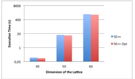
Figure 4.1: Comparison of SE++ with the optimized version of the algorithm.

Figure4.1shows the comparison between SE++ and the optimized SE++ algorithm (SE++ Opt). With these optimizations the execution time of SE++ is decreased by a factor of 11%. Despite of this improvement of the performance of SE++, we opted to compare the different algorithms (SE, SE++, ENUM and the Voronoi cell-based algorithm) without any optimization to avoid comparing versions of the algorithms with

(40)

4.1. SEQUENTIAL IMPLEMENTATIONS

Computed Nodes

Avoided Nodes

Figure 4.2: Representation of the symmetric subtrees whose computation can be avoided.

different levels of optimization, since it was not possible to optimize the others due to time restrictions. On the Voronoi cell-based algorithm we implemented, instead of storing the whole set of relevant vectors as described in (Agrell et al.,2002), we only store the shortest vector found at any given moment. Therefore, after each CVP call, the computed vector is compared to the best vector that was already found and updates it, if it is better. This optimization was used on the comparison with the other algorithms, since the amounts of memory used would be huge even for lattices in low dimensions.

4.1.2 Improved SE++

The SE++ algorithm, presented in (Agrell et al.,2002) and improved in (Ghasemmehdi and Agrell,2009), computes the whole enumeration tree, thereby computing several vectors that are symmetric of one an-other. Since the purpose of the algorithm is to find the shortest vector v of norm _{∥v∥, it is not relevant} whether v or−v is found, since v and -v have exactly the same norm. Therefore, the computation of one of these vectors can be avoided, thus reducing the number of vectors that are ultimately computed. Figure

4.2shows a representation of the symmetric subtrees that can be avoided.

The ENUM algorithm avoids these computations, by using a variable, called last_nonzero, which stores the largest index i of the coefficient vector u for which ui ̸= 0. For example, if ui = 0, but its

parent ui+1̸= 0, then all its subtrees have to be computed. On the other hand, there are only symmetric

subtrees on nodes where uj = 0, j = i, ..., n. As shown in Figure4.2, there are only subtrees whose

computation can be avoided on the left-most nodes of each level. Since u defines the subtree of each level that will be computed next, it is updated differently for nodes that contain symmetric subtrees than for nodes that do not contain them. On trees that contain symmetric subtrees, the value of uiis incremented,

searching only in one direction. On the other hand, on trees that do not have symmetric subtrees ui is

updated in a zigzag pattern, searching in both directions (positive and negative values of ui).

Each time the algorithm moves up on the tree and i ≥ last_nonzero, the variable is updated, indicating the new lowest level that contains symmetric subtrees. At the beginning of the execution,

last_nonzero is initialized to 1, the index of the leaves. Due to the similarities between both algorithms

(41)

CHAPTER 4. TOWARDS EFFICIENT IMPLEMENTATIONS

Algorithm 6: Improved SE++ algorithm

1 Input: n, H Output: û∈ Zn 2 C =∞; 3 i = n + 1; 4 d_j = n, j = 1, . . . , n; 5 dist_n+1 = 0; 6 E_n,j = 0, j = 1, . . . , n; 7 last_nonzero = 1; 8 LOOP do 9 if i̸= 1 then 10 //move down i = i− 1;

11 E_j_−1,i = E_j,i − y_jH_j,i, j = d_i, d_i −

1, . . . , i + 1;

12 u_i =round(E_i,i);

13 y_i = (E_i,i− u_i)/H_i,i; 14 ∆i =sign(yi);

15 dist_i = dist_i+1+ y2_i; 16 else

17 //update best vector

if disti ̸= 0 then

18 û = u;

19 C = dist₁; 20 i = i + 1;

u, ∆, y, E, dist, H); 22 while dist_i < C; 23 m = i; 24 do 25 if i = n then 26 return û; 27 else 28 //move up i = i + 1;

u, ∆, y, E, dist, H); 30 while dist_i ≥ C; 31 d_j = i, j = m, m + 1, . . . , i− 1; 32 for j = m− 1, m − 2, . . . , 1 do 33 if d_j < i then 34 d_j = i; 35 else 36 break; 37 goto LOOP