Nome
Luís Pedro Bidarra Fernandes
Endereço electrónico: [email protected] Número do Bilhete de Identidade: 14090100 Título dissertação
An integrated model for simulation of construction phasing of arch concrete dams Orientador(es):
Professor Miguel Azenha Professor João Pedro Couto
____________________________________________________ Ano de conclusão: 2015 Designação do Mestrado:
Mestrado Integrado em Engenharia Civil
1. DE ACORDO COM A LEGISLAÇÃO EM VIGOR, NÃO É PERMITIDA A REPRODUÇÃO DE QUALQUER PARTE DESTA DISSERTAÇÃO
Universidade do Minho, ___/___/______
Although a dissertation is, by its academic purpose, an individual work, there are contributions of diverse nature that cannot and should not be forgotten to be highlighted.
Thereby, I want to express my deepest gratitude to my scientific supervisor Prof. Miguel Azenha. Thanks for believing in me, the wise advices, the motivation, patience, interest, guidance, tireless availability, the dispended time, and above all, for the trust placed in me and consequent opportunities presented which allow me to grow in a professional and personal level. His remarkable knowledge of the concrete thermal problem, of BIM and dams constructive phasing revealed to be imperative for the delivery of this thesis. I also acknowledge the importance of Prof. João Pedro Couto for all the monitoring throughout the entire process. To my family, especially my Mother, my Grandmother, my aunt São, my uncle Nelo, my Father, my goddaughter Ana Sofia and my cousin Rui Miguel a huge thank you by your affection, by always believing in me and your selflessness with regards to me. To my departed grandfather Quim for all the love and courage conveyed throughout my life, to who I dedicate this work.
Also a word of appreciation to all my close friends I made during the academic path, I keep with much esteem the friendship here created and developed, a thank you all for the strength and will, who passed me and without which we often feel I should be lost.
The construction of dams and their constructive phasing are extremely complex activities, which lead to very high costs and thus require optimization. However, this type of optimization is only assessed by the constructor trying to evaluate alternative scenarios compared to reference scenarios proposed by the designer himself. In this sense it must be increasingly an attempt to approach the integrated project delivery (IPD) approaches advocated by BIM philosophies. The developed framework intends to integrate several valences in an automated way and supported in software tools combine various capacities both in terms of modeling BIM models, but also of thermal calculations and also defining construction phasing. It is precisely in this line that is intended this dissertation.
Therefore, in this study the main objective was the establishment of an integrated framework that would connect the modeling, the thermal calculation and dams constructive phasing according to an IPD. The developed framework will allow that an engineer in the design phase can already take into account a consequence weighted of alternatives and reference scenarios that are quickly investigated and let quickly combine the enormous impact that exists on decisions taken in very preliminary stages of the project.
In the dissertation are presented the three developed computational tools related to the dam’s modelling, the thermal calculation and the constructive phasing.
The dam was modelled through visual programming resorting to Dynamo, that in turn is interoperable with the others developed tools. The thermal analysis preconized by 2D finite difference with a non-linear heat generation and division between layers was implemented in MATLAB. The developed tool for the constructive phasing, equally implemented in MATLAB, is based in a cellular automata algorithm. Finally, is presented a proposed integrated framework containing all of these aspects and where are demonstrated its feasibility and utility.
KEYWORDS: Dams; Visual Programming; Thermal calculations; Constructive phasing; Integrated framework.
A construção de barragens e o seu faseamento construtivo são atividades extremamente complexas, que acarretam custos muito elevados e que assim requerem otimização. No entanto este tipo de otimização só é avaliado por parte do construtor que tenta estudar cenários alternativos em relação a cenários de referência propostos pelo próprio projetista. Nesse sentido impõe-se cada vez mais uma tentativa de aproximação às abordagens de Integrated Project Delivery (IPD) preconizadas pelas filosofias BIM, nomeadamente através da integração entre várias valências de uma forma automática e com suporte a ferramentas informáticas combinar várias capacidades, quer ao nível da modelação para obter modelos BIM, como também dos cálculos térmicos e da definição dos faseamentos construtivos. Tendo por base estes princípios foi elaborada esta dissertação.
Assim sendo, o principal objetivo deste trabalho consistiu no estabelecimento de um framework integrado que permite a ligação entre a modelação, o cálculo térmico e o faseamento construtivo de barragens, permitindo assim que um engenheiro na fase de conceção já consiga ter em conta uma consequência ponderada de alternativas e de cenários de referência que são rapidamente estudados e que permitem aliar o impacto sobre decisões que possam existir em fases muito preliminares do projeto.
Na dissertação são apresentadas três principais ferramentas desenvolvidas referentes à modelação da barragem, ao cálculo térmico e ao faseamento construtivo.
A barragem foi modelada através de programação visual com recurso ao Dynamo, que por sua vez é interoperável com as restantes ferramentas desenvolvidas. O cálculo térmico preconizado por diferenças finitas 2D com processo não linear de geração de calor e divisão entre camadas foi implementado no MATLAB. A ferramenta desenvolvida para o faseamento construtivo, igualmente implementada no MATLAB, é baseada num algoritmo de automação celular. No final apresenta-se uma proposta de um framework integrador contendo todos estes aspetos e onde é demonstrada a sua viabilidade e a sua utilização.
Palavras-Chave: Barragens; Programação Visual; Cálculo térmico; Faseamento construtivo; Framework integradora.
Introduction ... 1
Scope and motivation ... 1
Objectives ... 3
Outline of the thesis ... 4
Design, planning and construction of dams: classical approach and new challenges ... 5
Arch dam geometry... 5
Visual programming of dam body ... 7
2.2.1 History and definition of visual programming ... 7
2.2.2 Dynamo: a visual programming tool for parametric geometry modelling ... 9
Thermal control of concrete ... 12
2.3.1 Thermal cracking risk and thermal control in dams ... 12
2.3.2 Thermal problem of the concrete... 15
2.3.3 Heat transfer ... 15
2.3.4 Heat generation ... 22
2.3.5 Numerical Simulations ... 24
Planning and construction of dams ... 25
2.4.1 General remarks ... 25
2.4.2 Typical dam construction strategies ... 28
Visual Programming and modelling of an arch dam ... 31
Introduction ... 31
Case study of an arch dam ... 32
Visual programming applied to the case study ... 34
3.3.1 Arch dam body ... 35
Interoperability ... 46
Final considerations ... 48
Thermal analysis: implementation of a finite difference tool ... 49
Introduction ... 49
Intended inputs/outputs and operation of the developed tool ... 50
Discretization through the finite difference method ... 53
4.3.1 General nodes ... 55
4.3.2 Definition of the boundary conditions ... 56
Implementation of the computational tool ... 62
4.4.1 Explanation of the produced algorithm ... 62
Validation and demonstration of the developed tool ... 64
4.5.1 Validation ... 64
4.5.2 Demonstration ... 69
Final considerations ... 73
Proposal of method to generate construction dam schedules ... 75
Introduction ... 75
Definition of the hierarchy of dam’s construction planning rules ... 75
Cellular automata: from concept to implementation ... 77
5.3.1 Explanation of the produced algorithm ... 84
Implementation of the computational tool ... 88
Final considerations ... 90
Proposed framework for interoperability and implementation ... 93
Proposed framework ... 93
Examples of above framework related to the case study ... 99
6.1.1. Different concrete layers’ height with the use of pre-cooling ... 101
Discussion about the practical feasibility of this framework: ... 103
Conclusions ... 105
General conclusions ... 105
Future challenges ... 107
References ... 109
I. Appendix I – Produced code in dynamo ... 113
II. Appendix II – Generated Schedule for the case study ... 126
Figure 1-1 - MacLeamy curve. ... 2
Figure 2-1 - Arch dam terminology: a) Plan view; b) Central Cantilever. Adapted from (Pedro, 1999). ... 6
Figure 2-2 - Example of single and double-curvature dams. (U.S. Army Corps of Engineers, 1994). ... 7
Figure 2-3 - Draw a circle through a point using visual programming. ... 8
Figure 2-4 - The dynamo code and their results. (“Dynamo Primer,” 2015) ... 10
Figure 2-5 - Point dragged into dynamo workspace... 10
Figure 2-6 - Slider components and geometry preview ... 11
Figure 2-7 - Surface's vertices and edges. ... 11
Figure 2-8 - Alteration on surface's vertices coordinates ... 12
Figure 2-9 - Creation of parametric surface on dynamo ... 12
Figure 2-10 - Example of interior temperature distribution [ºC]. Adapted from (Li, Ren, Wu, & Zhao, 2008). ... 14
Figure 2-11 - Heat transfer mechanisms (Azenha, 2004). ... 16
Figure 2-12 – Elementary concrete element – adapted from (Bofang, 2014). ... 19
Figure 2-13 a) Heat generation rate as a function of αT; b) normalized heat generation rate f(αT) - (Azenha, 2009). ... 23
Figure 2-14 - Construction of Almendra Dam in Spain. (Iberdrola, 2014) ... 26
Figure 2-15 - Concreting schedule of an arch dam (developed downstream view). Adapted from (Spanish Commitee on Large Dams, 1990) ... 27
Figure 2-16 - Concreting works. Adapted from (Spanish Commitee on Large Dams, 1990).. 27
Figure 2-17 – Constructive phasing: a)Cabril; b)Alto Lindoso. (Batista, 1998; Teles, 1985) . 28 Figure 2-18 - Construction of Baixo Sabor Dam (August 2012). ... 28
Figure 2-19 - Alto Lindoso dam contraction joints. (Farinha, 2003) ... 29
Figure 3-1 - Shape defining functions. ... 32
Figure 3-3 - Dam's vertical joint configuration. ... 34
Figure 3-4 - Overall workflow towards modelling the case study dam. ... 35
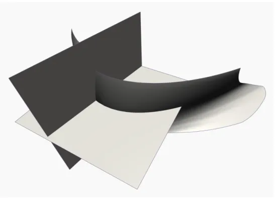
Figure 3-5 - Mesh Grid created for the medium sheet of the dam. ... 36
Figure 3-6 - NURBS curves. ... 36
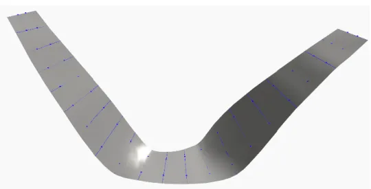
Figure 3-7 - Medium sheet of the arch dam. ... 36
Figure 3-8 - Created Dynamo node using Python. ... 39
Figure 1-9 - a) View of the upstream face of the dam's body; b) View of the downstream face of the dam's body. ... 39
Figure 3-10 - Points and lines picked from the dam's structural project. ... 40
Figure 3-11 - Planes intersection with the downstream and upstream surfaces of the dam. .... 41
Figure 3-12 - Modelling of the points and lines withdrawn from structural project. ... 41
Figure 3-13 - Surface of intersection of the dam's body and the ground. ... 42
Figure 3-14 - Dam's views: a) Upstream; b) Downstream. ... 42
Figure 3-15 - Points used to model the dam's galleries. ... 43
Figure 3-16 – Curves used to model the dam’s galleries. ... 43
Figure 3-17 - Adopted modelling phases in order to model the dam's galleries. ... 44
Figure 3-18 - Views of dam's galleries. ... 44
Figure 3-19 - a) Dam's view from left bank; b) Dam's view from right bank. ... 44
Figure 3-20 – Dam with the galleries modelled. ... 45
Figure 3-21 - Custom node created to cut the dam's body by horizontal planes. ... 46
Figure 3-22 - Views of the dam: a) sliced downstream view; b) sliced right bank view. ... 46
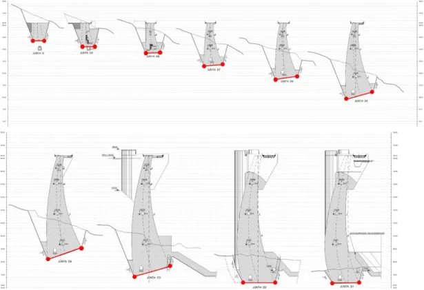
Figure 3-23 - Dam elevation and vertical profiles. ... 47
Figure 3-24 - IFC file open on Solibri Model Checker. ... 48
Figure 4-1 - Simplification introduced in the developed program: a) Real dam's shape; b) Adopted dam's shape. ... 50
Figure 4-5 - Schema adopted for the 2D algorithm. ... 53
Figure 4-6 - Types of nodes on a finite difference mesh. ... 54
Figure 4-7 - Local coordinate system used for the internal points. ... 55
Figure 4-8 - Coordinate system for the east points. ... 57
Figure 4-9 - Local coordinate system used for the north nodes. ... 58
Figure 4-10 - Local coordinate system used for the northwest corner node. ... 59
Figure 4-11 - Three point square mesh for one concrete layer. ... 60
Figure 4-12 - Changes scheme to make the equation evolutionary. ... 62
Figure 4-13 - Three point square mesh for two concrete layers. ... 62
Figure 4-14 - Element used for validation. ... 65
Figure 4-15 - Heat generation parameters ... 65
Figure 4-16 - Point of the element were the temperature were studied (crossed dot). ... 66
Figure 4-17 - Evolution of the temperature along time – Validation 1. ... 66
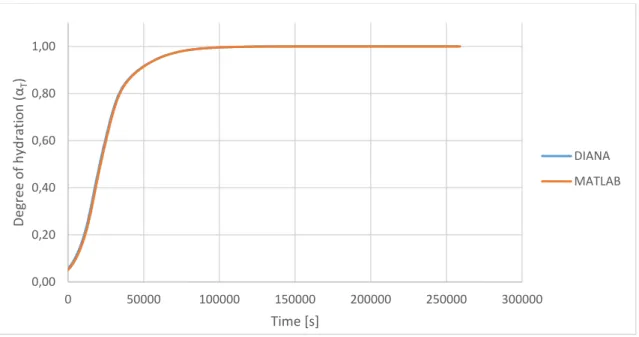
Figure 4-18 - Evolution of the degree of hydration along time – Validation 1. ... 67
Figure 4-19 - Points of the model were the temperature were studied (crossed). ... 68
Figure 4-20 - Evolution of the temperature along time – Validation 2. ... 68
Figure 4-21 - Temporal gradient for the middle center points of the concrete layers. ... 70
Figure 4-22 - Temporal gradient for the middle lateral points of the concrete layers. ... 71
Figure 4-23 - Temporal gradient of the boundaries between concrete layers. ... 71
Figure 4-24 - Spatial gradient for a representative layer. ... 72
Figure 4-25 - Temperature maps for three different time instants. ... 73
Figure 5-1 - Minimum time between concreting successive layers. ... 76
Figure 5-2 - Maximum difference of heights between adjacent layers. ... 76
Figure 5-3 - Maximum time between concreting successive layers. ... 77
Figure 5-5 - One dimensional cellular automata grid. ... 78
Figure 5-6 - One dimensional cellular automata states. ... 79
Figure 5-7 – Neighborhood for the central cells... 79
Figure 5-8 - Neighborhood for the corner cells. ... 79
Figure 5-9 – Possible central cells neighborhood configurations – cell itself in green and the neighbors in red. ... 79
Figure 5-10 – Possible corner cells neighborhood configurations – cell itself in green and the neighbor in red. ... 79
Figure 5-11 - Neighborhood possible outcomes for the central cells – cell itself in green and the neighbors in red. ... 80
Figure 5-12 - Neighborhood possible outcomes for the corner cells – cell itself in green and the neighbors in red. ... 81
Figure 5-13 - One dimensional cellular automata for the first ten time steps. ... 81
Figure 5-14 - Example of a game of life pattern. ... 83
Figure 5-15 - Cellular automata propagation over time. (Adamatzky, 2010) ... 83
Figure 5-16 - Used grid for the cellular automata algorithm. ... 84
Figure 5-17 - First concreting steps. ... 85
Figure 5-18 – Available concreting positions for step 2. ... 85
Figure 5-19 – Concreted layers after the second step. ... 86
Figure 5-20 - Available concreting positions until the step 6... 86
Figure 5-21 - Concreted layers after the seventh step. ... 87
Figure 5-22 - Concreted layers after the third step. ... 87
Figure 5-23 – Elevation of the dam modeled in chapter 3. ... 88
Figure 5-24 - Used grid in the cellular automata algorithm. ... 89
Figure 6-1 - Proposed framework. ... 94
Figure 6-2 - Proposed framework subset 1 – see Figure 6-1. ... 95
Figure 6-6 - Proposed framework – see Figure 6-1. ... 99
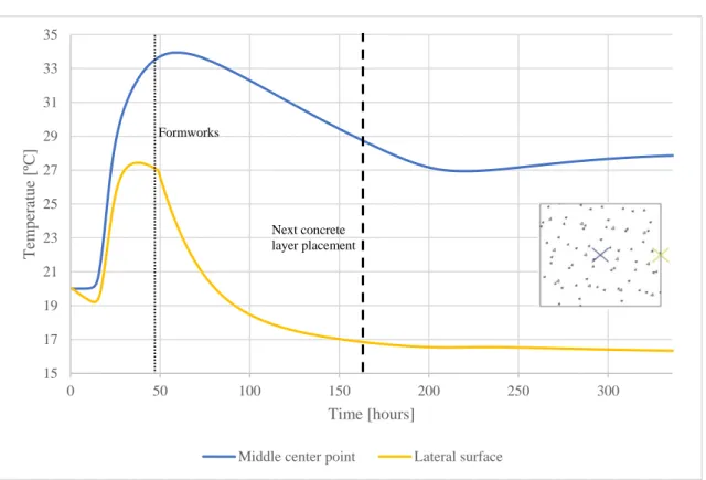
Figure 6-7 – Temperature evolution over time in the boundaries between layers for the example 1 simulation. ... 100
Figure 6-8 - Temperature evolution over time in the middle center points of the concrete layers for the example 1 simulation. ... 100
Figure 6-9 - Temperature evolution over time in the middle lateral points for the example 1 simulation. ... 101
Figure 6-10 – Spatial gradient for the example 1 simulation. ... 101
Figure I-1 - Overview of the produced dynamo code. ... 113
Figure I-2 - Overview of the code in section 1 (see Figure I-1). ... 114
Figure I-3 - Code used to model the dam's medium sheet (section 1.1 - see Figure I-2). ... 114
Figure I-4 - Code used to give thickness to dam's medium sheet (section 1.2 - see Figure I-2). ... 115
Figure I-5 - Generation of dam's body solid (section 1.3 - see Figure I-2). ... 115
Figure I-6 - Cut of the dam's solid by the left and right banks (section 1.4 - see Figure I-2). 115 Figure I-7 - Overview of the code in section 2 (see Figure I-1). ... 116
Figure I-8 - Definition of the vertical planes that represent the vertical construction joints (section 2.1 - see Figure I-7). ... 117
Figure I-9 - Definition of one of the lines that will be used to create the surface on intersection of the dam with the ground (section 2.2 - see Figure I-7). ... 117
Figure I-10 - Creation of the surface on intersection of the dam with the ground and split the dam's body by the created surface (section 2.4 - see Figure I-7). ... 118
Figure I-11 - Overview of the code in section 3 (see Figure I-1). ... 119
Figure I-12 - Creation of the NURBS curve parallel of the medium sheet in all the dam's galleries (section 3.1 - see Figure I-11). ... 120
Figure I-13 - Overview of the code used to model one dam gallery (section 3.2 - see Figure I-11). ... 120
Figure I-14 - Creation of the solid with an exaggerated height that will be used to model the dam's galleries (section 3.3- see Figure I-11). ... 121
Figure I-15 - Creation of the surface of the top of the dam's gallery and cut of the previously
created solid (section 3.4 - see Figure I-11). ... 121
Figure I-16 - Union of the four dam's galleries and subtraction of these to the dam's body solid (section 3.5 - see Figure I-11). ... 122
Figure I-17 - Overview of the code in section 4 (see Figure I-1). ... 122
Figure I-18 - Definition of the number of vertical planes that represent the dam's construction joints and will vertically slice the dam's body (section 4.1 - see Figure I-17). ... 123
Figure I-19 - Definition of the horizontal planes that will slice the dam's body according with a given concreting layer height (section 4.2 - see Figure I-17). ... 123
Figure I-20 - Code used to slice the dam's body by the previously defined horizontal planes (section 4.3 - see Figure I-17). ... 123
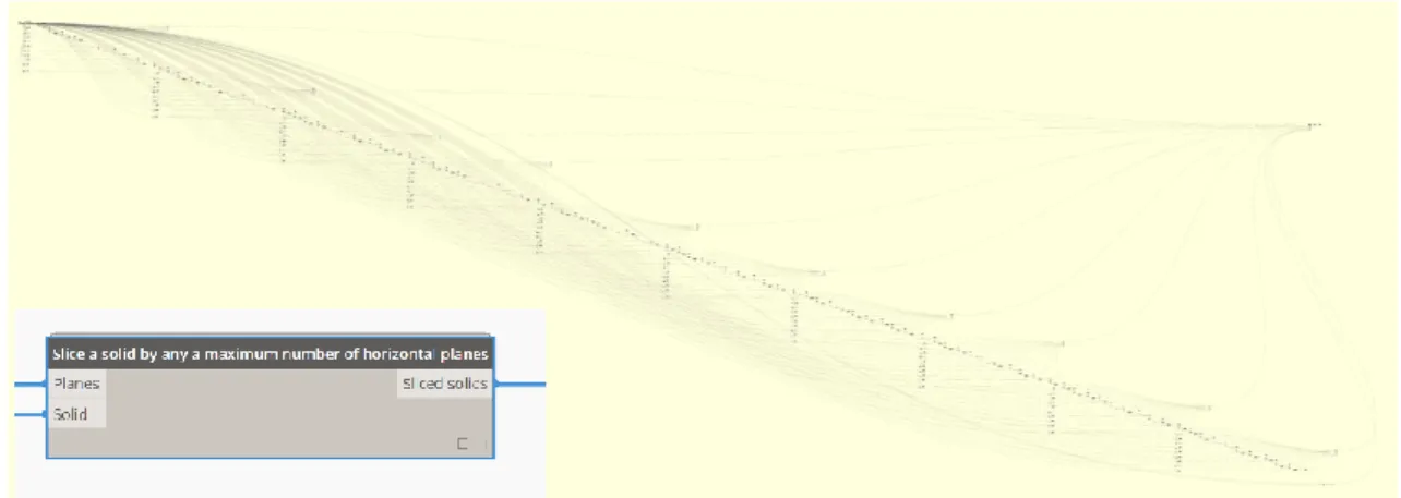
Figure I-21 – Overview of the custom node created to cut the dam's body by any number of horizontal planes (Section 4.4 - see Figure I-17)... 124
Figure I-22 - Zoom at the created algorithm to create to cut the dam's body by horizontal planes (see Figure I-21 and Figure I-17). ... 124
Figure I-23 - Import of all the construction blocks to Autodesk REVIT (section 4.6 - see Figure I-17). ... 125
Figure I-24 - Developed code in Dynamo for the introduction of the non-geometrical information in the model. ... 125
Figure II-1 - Dam construction schedule for the case study dam. ... 126
Figure II-2 - Waiting times between concreting successive layers. ... 127
Table 2-1 - Adopted heat parameters (per Kg of cement) (Azenha, 2009). ... 24
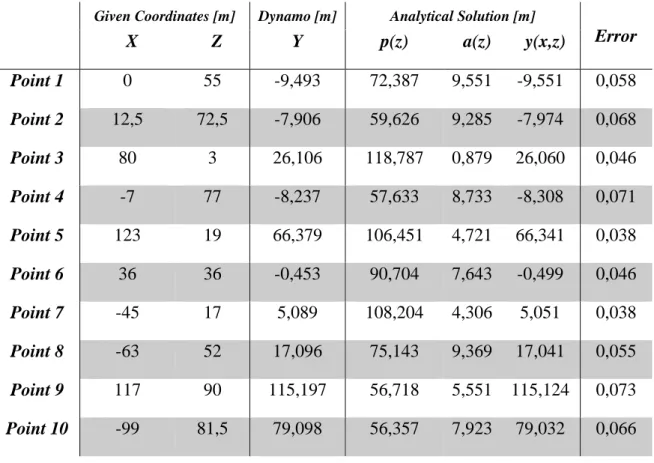
Table 3-1 - Comparison between dynamo and analytical solution coordinates for the used mesh. ... 37
Table 3-2 - Comparison between dynamo and analytical solution coordinates for a mesh of points spaced by 1 meter. ... 38
Table 4-1 - Developed program inputs ... 63
Table 6-1 - Studied parameters for the studied scenarios. ... 102
Table III-1 - Exchange Requirement 1. ... 129
Table III-2 - Exchange Requirement 2. ... 129
Table III-3 - Exchange Requirement 3. ... 129
Table III-4 - Exchange Requirement 4. ... 130
CHAPTER 1
INTRODUCTION
Scope and motivation
The analysis of the behavior of the concrete during the first ages is covered of an great importance in multiples dominium’s, among which it could be referred which aims to avoid the cracking related to the thermal problem due to the heat of hydration of the concrete (Azenha, 2004).
The study of the concrete temperature of hydration is especially important at the concreting of the concrete pieces of large dimensions or too thick, or in concretes with considerable percentage of cement, from which the differential of the temperature due by the heat of hydration it’s the fact prepondering to the premature cracking of concrete.
By the motive enunciated above it became needed to dispose of methodologies of analysis of the evolution of the temperature of the concrete along the time that requires the mobilization of calculus processes.
Due to the problem complexities, especially in mass-concrete works as dams, a common practical between the projectors is the search to control the cracking risk impounding maximum concrete layers height or establishing minimum waiting times between concreting successive layers. This measures are taken aiming a more speed-up dissipation of the generated heat, in order to avoid a very sharp elevation of the temperature of the concrete element. However, once the cracking risk depends on a large set of factors beyond the geometrical conditions (concrete mix, ambient temperature, initial temperature of the concrete, boundaries conditions), it is understood that the commonly established rules in the contract documents turn out to be conservative, translating accumulated experience or prescriptions that normally lead to positive results.
So, it’s relevant, in addition to the thermal-mechanical calculation of the concrete element, the utilization of methodology that allows the constructive phasing of dams. In this context it’s pertinent the development of methodologies that permit an optimization of this processes that leads to an improvement of the planned construction schedule and associated costs.
The aforementioned problematics are related to mass-concrete works, as the dams’ construction, which are large structures with complex shapes, whose modelling is a very difficult process through traditional modeling tools, thereby, it’s interesting the use of advanced modeling tool, as the visual programing in order to obtain a parametric model that could assist and improve the design procedures of arch dams from early stages of development.
The dam’s modelling, the thermic problem and the constructive phasing could be integrated in a framework based in the Integrated Project Delivery approaches advocated by BIM philosophies. Integrated Project Delivery (IPD) is a project delivery approach that integrates practices into a collaborative process to optimize project results and maximize efficiency through all phases of design and construction. (Aia, 2007)
The IPD based framework intends to anticipate the design efforts and by this way, making the design decisions earlier when opportunity to influence positive outcomes is maximized and the cost of changes minimized. The IPD is supported on the “MacLeamy Curve ” presented in Figure 1-1, where is noticeable the gains in using the IPD.
Figure 1-1 - MacLeamy curve.
Hence, it’s important to develop a framework the helps the dam design in their early stages of the project and thus allows the choice for the best construction scenario through the study of multiple construction scenarios alternative scenarios.
Objectives
The aim of this work is to address the challenges and opportunities that are posed to the early stages of design of the dam’s projects: (i) the availability of software capable of modelling complex geometries, (ii) perform fast pre-design thermal calculations and (iii) easily study alternative construction scenarios.
In what regards to the modelling of complex structures the main objective is model an arch dam complex double curvature shape and the minor objectives are centered in the modeling some of the dam’s details, as for example the intersection with the underling terrain and the dam’s galleries. Another important aspect to explore are the interoperability of the created BIM model with another BIM platforms and with the developed computational tools.
In what refers to the thermal analysis the major objective is the development of a computational tool that allows the performing of the need thermal calculation to pre-design stage of a dam project. In a more specific way, the achievement of the aforementioned objective is pursued by a set of partial objectives which includes the derivation of heat conducting equations that support the thermal calculations, simulation of the layered construction phasing, the heat conduction inside the concrete, the heat convection with the surrounding environment, with due consideration of the effects of formwork and their withdrawal and the non-linear heat generation of concrete. The developed computational tool must also be capable of automatically generating temperature maps and plots of temperature evolution for selected relevant instants over time.
Relatively to the study of the dam’s constructive scenarios the objective is the development of a computational tool that allows quick study of different construction scenarios. To achieve the above-mentioned objective a set of partial objectives were defined, which consist find a set of rules that materialize the usual dam’s planning, implement a decision-taking algorithm capable of perform the desired planning.
Lastly, it is intended to propose an integration of the modelling of the dam and the developed computational tools in a framework increasing the efficiency of use of developed works. The proposed framework will allow to compare different construction scenarios and will allow the best decision-making for the economical and fastest one.
Outline of the thesis
This dissertation is organized in seven chapters, the first of which consists of this introduction. In chapter 2 is presented the literature review about the themes addressed in this dissertation. The first addressed theme was the complex shape of arch dam, the challenges and opportunities that advanced modelling methodologies as the visual programming and parametric modelling present to these hydraulic structures. The following was addressed the thermal problem in mass concrete structures, passing by the processes of transfer and heat generation, as well as the adverse effects that may arise, such as the premature thermal cracking of the concrete and the measures to prevent these risks either on site or by numerical simulations. The last theme addressed was the typical methods of dam’s construction and planning.
In chapter 3 were made the modelling of the dam following the line of visual programming using Dynamo. This way was made the modeling of the dam’s body, their intersection with the underlying terrain and its galleries. Finally, were made yet, the division of dam’s body by horizontal and vertical joints.
Chapter 4 is related to the thermal analysis on dam’s. Along this chapter are derivated the finite difference equations that support the development of a computational tool and its implementation. Are also presented multiple program validations.
In chapter 5 were proposed a method to generate construction dam schedules, following a pre-established set of rules, by the implementation of a cellular automata algorithm. Along this chapter the developed computational tool was used to test multiple construction scenarios. Chapter 6 propose a framework that integrates the proceedings developed in the previous three chapters.
To conclude, chapter 7 provides a summary of the main conclusions and some suggestions for possible extensions of the conducted work.
CHAPTER 2
DESIGN, PLANNING AND CONSTRUCTION OF DAMS:
CLASSICAL APPROACH AND NEW CHALLENGES
Arch dam geometry
According to (USDI, 1977) an arch dam is a solid concrete dam, curved upstream in plan. A large part of the stability results by transmitting the the water pressure and other loads by arch action into the canyon walls additionally to resisting part of the pressure of the reservoir by its own weight.
A good structural behavior of an arch dam in face of actions requires a monolithic structure, and special care in the construction to guarantee that no structural discontinuities, as open joints or cracks, occur when the structure dam assumes its water load.
The complete design of a concrete arch dam includes not only the determination of the most efficient and economical proportions for the water impounding structure, but also the determination of the most suitable appurtenant structures for the control and release of the impounded water consistent with the purpose or function of the project.
Arch dams are commonly classified as thin, medium-thick, or thick arch dams. This relation is obtained with a b/h ratio, where b is the base thickness of the crown cantilever and h is the structural height of the dam. So a thin arch is defined as an arch dam with a b/h of 0.2 or less, a medium-thick arch dam is defined as an arch dam with b/h ratio between 0.2 and 0.3 and a thick arch dam is an arch dam with a b/h ratio of 0.3 or greater.
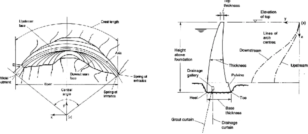
The type of arch dams is essential defined as two category of sections, commonly arch section and cantilever section (U.S. Army Corps of Engineers, 1994), as presented in Figure 2-1. Therefore, the faces of the cantilever units are referred as upstream and downstream and the matching arch faces are Extrados and Intrados, as appropriate.
The canyon walls could have schematic profiles of various dam sites, formed in “V” or “U”. A Narrow-V site is related to canyon walls generally straight, with few undulations, and converge to a narrow streambed. This type of site is favored for arch dams since the applied load will be transferred to the rock predominantly by arch action. Another “V” form is a Wide-V, being the principal difference for the previous “V” is that the arch would be thicker. In wide-V the canyon walls will have more pronounced undulations but will be generally straight after excavation, converging to a less pronounced v-notch below the streambed.
According to (Pedro, 1999; U.S. Army Corps of Engineers, 1994), an arch dam may be classified as single curvature or double curvature in plan.
Single curvature arch dams are curved in plan only, as shown in Figure 2-2. Vertical sections, or cantilevers, have vertical or straight sloped faces, or may also be curved with the limitation that no concrete overhangs the concrete below. Overhang refers to the concrete on the downstream face where the upper portion overhangs the lower portion. Overhang is most at the crown cantilever, gradually diminishing toward the abutments. The single curvature is normally use in arch gravity dams with thick vaults.
Double curvature arch dams means the dam is curved in plan and elevation as shown in Figure 2-2. This type of dam utilizes the concrete weight to greater advantage than single-curvature arch dams. Consequently, less concrete is needed resulting in a thinner, more efficient dam.
a) b)
Figure 2-1 - Arch dam terminology: a) Plan view; b) Central Cantilever. Adapted from (Pedro, 1999).
The double curvature dams are used to arch dams with thin shells or domes, with a vertical and horizontal curvature as shown in the Figure 2-2.
Figure 2-2 - Example of single and double-curvature dams. (U.S. Army Corps of Engineers, 1994).
The main loads to be considered in dams are: the reservoir and tailwater, the temperature, the internal hydrostatic pressures, the dead load and the earthquake. (USDI, 1977).
In the scope of the present work will be addressed the temperature loads that are imposed on a concrete dam when the concrete undergoes a temperature change and volumetric change is restrained. The magnitude of the temperature load is related to the closure temperature, to the thermal coefficient of expansion of the concrete, and to the temperature difference between the closure temperature and the operating temperatures. (Townsend, 1965).
Visual programming of dam body
2.2.1 History and definition of visual programming
Visual programing, among other things, it’s mainly utilized for the generation of geometry through parametric modeling.
Modeling frequently involves establishing visual, systemic, or geometric relationships between the parts of a model. Many times, these relationships are developed by workflows ranging from
concept to result by way of rules. When modeling, without knowing, the user is working algorithmically - defining a step-by-step set of actions that follow a basic logic of input, processing, and output. Programming allows to continue to work this way but by formalizing algorithms. Algorithms can generate any kind of complex geometries.
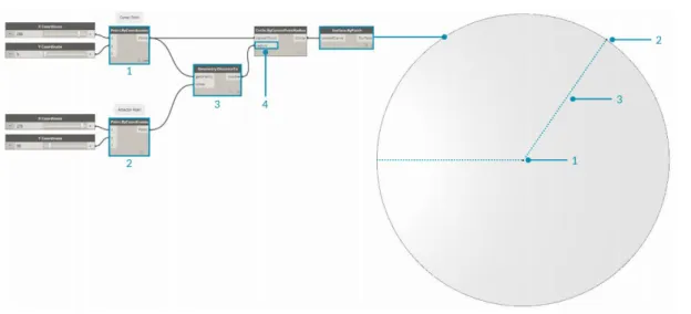
The process is essentially the same for both Programming and Visual Programming. They utilize the same framework of formalization. However, in visual programming we define the instructions and relationships of our program through a graphical (or "Visual") user interface. Instead of typing text bound by syntax, we connect pre-packaged nodes together. Then is presented a comparison of the same algorithm - "draw a circle through a point" - programmed with nodes versus python programming language code:
Visual Program:
Figure 2-3 - Draw a circle through a point using visual programming.
Textual Program: myPoint = Point.ByCoordinates(0.0,0.0,0.0); x = 5.6; y = 11.5; attractorPoint = Point.ByCoordinates(x,y,0.0); dist = myPoint.DistanceTo(attractorPoint); myCircle = Circle.ByCenterPointRadius(myPoint,dist);
Visual programing, among other things, it’s mainly utilized for the generation of geometry through parametric modeling.
Parametric modeling is a modeling methodology that become especially relevant in early nineties with the creation of the first commercial successful parametric software,
of making design changes ought to be as close to zero as possible” (Geisberg quoted in:
(Teresko, 1993)).
Geisberg highlights two points. The first is that parametric modelling should enable designers to explore a variety of designs (Teresko, 1993) and the second point is that parametric models allow choices to be made later in the design process.
Since nineteen ninety parametric modeling was used by mechanical and aerospace engineers. This methodology of modeling is based upon the creation of algorithms capable of generating models fully controlled by a reduced number of parameters. (Azenha, Lino, & Caires, 2015) Through use of this modeling methodology, the user is able to create any kind of complex geometry easily and recognize the influence of each parameter in the model. Thus, it is easier and intuitive to make changes to the parameters to the final model in order to achieve the desired result.
The exploitation of this methodology is interesting to the modelling of complex structures as concrete arch dams, due to their double curvature shape.
2.2.2 Dynamo: a visual programming tool for parametric geometry
modelling
Dynamo falls in the Visual Programming paradigm, although the textual programming is possible in the application as well. Dynamo is a visual programming tool that aims to be accessible to both non-programmers and programmers alike. It gives users the ability to visually script behavior, define custom pieces of logic, and script using various textual programming languages.
Dynamo will enable the user to work within a Visual Programming process wherein he connects elements together to define the relationships and the sequences of actions that compose custom algorithms. The user can use their algorithms for a wide array of applications - from processing data to generating geometry - all in real-time and without writing any code.
Figure 2-4 - The dynamo code and their results. (“Dynamo Primer,” 2015)
Simple example of visual programming
To better understand how to use dynamo and its visual programming language, one detailed example will be given of how to create a parametric surface model.
The first step to creating a parametric surface model, is the creation of points which will be the surface’s vertices. Using a node for creating a point, three inputs are needed, corresponding to the x-coordinate, the y-coordinate and the z-coordinate, similar to presented in Figure 2-5. In this case the inputs may be any real number and can be introduced by using a slider node. The slider node allows the creation of any number in a range defined by the user, for example, integers ranging from 0 to 10. The sliders can be connected to the point node’s inputs thus outputting a three-dimensional point in dynamo with the desired coordinates as presented in Figure 2-6.
Figure 2-6 - Slider components and geometry preview
These nodes can be copied in order to create the three additional vertices of the surface. The surface’s vertices will be connected by lines which will form the surface’s edges.
Figure 2-7 - Surface's vertices and edges.
Any adjustment in the values of the point’s coordinates will automatically be reflected onto the geometry as presented on Figure 2-8.
Figure 2-8 - Alteration on surface's vertices coordinates
After the creation of surfaces, vertices and edges, the surface can be created using the create surface by patch node that create a surface between closed curves as seen on Figure 2-9.
Figure 2-9 - Creation of parametric surface on dynamo
Thermal control of concrete
2.3.1 Thermal cracking risk and thermal control in dams
Mass concrete structures produce significant temperature differentials between the interior and the outside surface of the structures. Mass concrete is defined by American Concrete Institute Committee 207 as “any volume of concrete with dimensions large enough to require that measures be taken to cope with the generation of heat from hydration of cement and the respective volume change to minimize cracking.”.
The proper design and construction of mass concrete dams can help prevent disasters due to the thermal cracking of concrete. To ensure safety and durability, mass concrete have attracted increasing attention in the structural design and construction. (Kim, 2010)
The main difference between mass concrete dam construction and other typical concrete structure types is its thermal behavior. Cracking in mass concrete structures is undesirable because it affects the water tightness, internal stresses, durability, and the appearance of these structures. Cracking will occur when the developed tensile stresses exceed the concrete tensile strength. These tensile stresses may occur because of imposed loads on the structure, but more often occur because of restraint against volumetric change. The largest volumetric change in mass concrete results from change in temperature. (USDI, 1977)
The cracking tendencies occur with high thermal gradient between the center and the surface, when the thermal stress in concrete exceeds its tensile strength. The cracking can be reduced to acceptable levels, in most instances, by the use of appropriate design and construction procedures.
Thus, temperature control measures are employed in mass concrete dams to facilitate construction of the structure, minimize and/or control the size and spacing of cracks in the concrete, and permit completion of the structure during the construction period, because minimizing volumetric changes makes also possible the use of larger construction blocks, thereby resulting in a more rapid and economical construction.
The thermal control could be made through numerical simulation of the temperatures inside the concrete, obtaining temperature maps as presented in Figure 2-10. The important factor to prevent cracking is the thermal stresses inside concrete and not the temperatures, because the thermal stresses are not only related with the temperatures, but with the restraints of the concrete element. Traditionally only the temperature is considered in the early stages of development of the project, because the temperature gradients are a good indicator of the thermal stresses generated inside the concrete for that stage of development of the project.
Figure 2-10 - Example of interior temperature distribution [ºC]. Adapted from (Li, Ren, Wu, & Zhao, 2008).
The most common methods of temperature control, are the precooling that is the most effective temperature control, which reduces the placing temperature of the concrete.
Methods of reducing the placing temperature range from restricting concrete placement during the hotter part of the day or the hotter months of the year, to a full treatment of refrigerating the various parts of the concrete mix to obtain a predetermined, maximum concrete placing temperature.
The refrigeration of the concrete mix includes the cooling of the water in the concrete mix, the cooling of the aggregates and addition of ice to the concrete mix. (Bofang, 2014)
Another method of minimizing the concrete temperatures are the reduction of the amount and type of cement or adding pozzolan materials to reduce the heat hydration reaction of cement. (Spanish Commitee on Large Dams, 1990)
2.3.2 Thermal problem of the concrete
The analysis of the behavior of concrete in the first ages requires the knowing of his origin. (Azenha, 2004)
The water addition in concrete starts the hydration reaction that is responsible for the development of the mechanical properties of the concrete. The chemical reactions related to the concrete hydration are exothermic, with great heat generation.
The heat generation causes a temperature rise in concrete, which becomes higher than the surrounding environmental temperature. Thereby, heat transfer between concrete and the surrounding environment starts through the mechanism of convection. During the period while the amount of heat generated is greater than the amount of heat transferred between the concrete and the environment, the temperature in the concrete element keeps rising, with the core of the element standing hotter than the external surfaces. At some point in time, the heat generated by the chemical reaction equals the heat transferred to the surrounding environment. From this instant the concrete element starts cooling until it attains thermal equilibrium with the environment, which represents the end of the thermal problem related to the heat of hydration of cement. This thermal equilibrium rely on element size, shape, the concrete composition, the initial concrete temperature and environmental temperature, (Bofang, 2014).
This temperatures differentials in the concrete generate a volumetric expansion, when the temperatures are rising, followed by and contraction, when the temperatures are dropping, that in presence of external or internal restrictions could cause cracking of the concrete.
2.3.3 Heat transfer
Before proceed, it’s important the identification of the phenomena and the parameters involved in the characterization of a mass thermal behavior.
The heat transfer consists in the movement of thermal energy due to temperature differentials. Thus, when occur temperature differentials there are conditions for heat transfer.
In the thermal study of concrete in the first ages, the heat transfer could occur from different natures: conduction, convection or radiation (Figure 2-11), (Azenha, 2004; Kim, 2010). The temperatures distribution in a mass is, indeed, controlled by the combination of those three mechanisms, it’s not possible isolate completely one mechanism from their interactions with
the remaining. However it’s usual the separation of the heat transfer mechanisms, which does not involve significant errors (M. N. Ozisik, 1985) and simplifies the analysis.
Figure 2-11 - Heat transfer mechanisms (Azenha, 2004). The three heat transfer mechanisms aforementioned are described next.
Internal heat transfer by conduction
Conduction is the process of heat transfer wherein the exchange in thermal energy is made by the random movement of molecules or by the movement of free electrons. It is the typical process of heat transfer inside a solid (Azenha, 2004, 2009; Kim, 2010). One example of heat transfer by conduction is the case of concreting of a concrete piece adjacent the other previously existing. The heat generated by the reactions of hydration of a newly concreted piece will be transmitted by conduction to the existing piece through their physical boundaries.
The heat conduction in a solid could occur in steady-state regime (when the temperature in any point don’t changes along the time), or in variable regime (with the temperature variations in the time).
Conduction on steady-state regime
The empirical equation of heat conduction is based in experimental observations and its governed by Fourrier’s law, that for the one-dimensional case on steady-state conditions is:
𝒒𝒙′′= 𝒒𝒙
𝑨 = −𝒌
𝝏𝑻
Where:
𝑞𝑥′′ – heat flow through a surface by area unity (W/m2)
𝑞𝑥 – heat flow (W);
𝐴 – area crossed by the heat flow (m2);
𝑘 – thermal conductivity (W/m K); 𝑇 – temperature (K);
𝑥 – coordinate (m).
The signal (-) in the equation is related to the fact of the flow occur towards decreasing temperatures.
According to equation [2.1], the heat flow direction will always be perpendicular to the isothermal surface.
Taking in account that a solid is constituted by free electrons and atoms connected according a periodic arrangement (atomic mesh), the transmission of thermal energy by conduction occurs in two ways: by movement of free electrons and by vibrating waves propagating through the atomic mesh. These effects are additive, and 𝑘 is the result of the sum of the electric and the mesh components. In nonmetallic solids (like the constituents of fresh concrete) the value of 𝑘 its conditioned mainly by the mesh component, which depends on the frequency of the interaction between the constituents. The regularity of the mesh arrangement affects the thermal conductibility by the following way: crystalline materials (well-ordered meshes) have bigger values of 𝑘 than amorphous materials like the glass (Incropera & DeWitt, 2001).
For utilization in multidimensional means the Fourrier’s law generalizes by the vectorial representation 𝒒𝒙′′ = −𝒌𝛁𝑻 = −𝒌 (𝓲 𝝏𝑻 𝝏𝒙+ 𝓳 𝝏𝑻 𝝏𝒚+ 𝓴 𝝏𝑻 𝝏𝒛) [2.2]
where:
𝑥, 𝑦, 𝑧 – coordinates in the reference axis system; 𝒾, 𝒿, 𝓀 – inverters of the reference axis system.
It’s implicit in the equation [2.2] that the heat flow is always perpendicular to isothermal surfaces.
Conduction in variable regime
The Fourrier’s law is applicable to the conduction of heat in variable regime, for which the temperature distribution evolves along time until the equilibrium point is reached. It is important, before anything else, to retain some remarks about the heat conduction to better understand the heat conduction phenomes in variable regime: the specific heat, the specific volumetric heat and the thermal diffusibility (Azenha, 2004).
The specific heat c is the quantity of heat necessary to rise a unity of mass of a body by one unity of temperature; it’s expressed in J / (Kg K).
The specific volumetric heat ρc results from the product of the specific heat by specific mass of the material (ρ), it’s usually utilized to represent the material capacity to store energy; the
unities in which it is expressed are J/(m3 K).
The relation between the thermal conductibility and the specific volumetric heat it’s called
thermal diffusibility αT (m2/s)
𝜶𝑻=
𝒌
𝝆𝒄 [2.3]
witch represents a measure of the capacity of a material to conduct thermal energy in relation
to their ability to store it. Materials with elevate αT respond quickly to thermal changes in the
surrounding environment, taking less time until the attain point is established.
The main objective of a conduction analysis is determinate the temperatures inside an element, as result of boundary conditions and heat generation due cement hydration. For that purpose, is
used the Fourrier’s equation that is based on the Fourrier’s law. For aiding the following deduction let’s consider the representative elementary volume (REV) presented in Figure 2-12.
Figure 2-12 – Elementary concrete element – adapted from (Bofang, 2014).
In the presence of temperature differentials between the REV surface and the REV core it will be heat convection through faces of the REV, in perpendicular directions to the correspondent surfaces. In three faces of the element with different directions the heat fluxes could be
identified by qx, qy and qz. In the opposite faces, the heat fluxes can be represented in Taylor’s
series expansion by:
𝒒𝒙+𝝏𝒙= 𝒒𝒙 +𝝏𝒒𝒙 𝝏𝒙 𝒅𝒙 [2.4] 𝒒𝒚+𝝏𝒚 = 𝒒𝒚+𝝏𝒒𝒚 𝝏𝒚 𝒅𝒚 [2.5] 𝒒𝒛+𝝏𝒛 = 𝒒𝒛+𝝏𝒒𝒛 𝝏𝒛 𝒅𝒛 [2.6]
According to the First Law of Thermodynamics in a closed system we have:
𝑬̇𝒈= 𝑸̇ 𝒅𝒙 𝒅𝒚 𝒅𝒛 [2.8] 𝑬̇𝒔𝒕= 𝝆𝒄 𝝏𝑻 𝝏𝒕𝒅𝒙 𝒅𝒚 𝒅𝒛 [2.9] Where:
𝐸̇𝑖𝑛 – is the entrance energy rate (W);
𝐸̇𝑜𝑢𝑡 – is the exit energy rate (W);
𝐸̇𝑔 – is the generation energy rate (W);
𝐸̇𝑠𝑡 – is the storing energy rate (W);
𝑄̇ – is the energy generation rate by volume unit (W/m3);
𝑡 – is the time (s);
Thus, considering the heat fluxes in concrete element faces that are represented by 𝐸̇𝑖𝑛 and 𝐸̇𝑜𝑢𝑡,
and substituting in the equations [2.7] and [2.8] in [2.9]:
𝒒𝒙+ 𝒒𝒚+ 𝒒𝒛+ 𝑸̇ 𝒅𝒙 𝒅𝒚 𝒅𝒛 − 𝒒𝒙+𝝏𝒙− 𝒒𝒚+𝝏𝒚− 𝒒𝒛+𝝏𝒛= 𝝆𝒄 𝝏𝑻 𝝏𝒕𝒅𝒙 𝒅𝒚 𝒅𝒛 [2.10] Substituting [2.4], [2.5] and [2.6] in [2.10]: −𝝏𝒒𝒙 𝝏𝒙 𝒅𝒙 − 𝝏𝒒𝒚 𝝏𝒚 𝒅𝒚 − 𝝏𝒒𝒛 𝝏𝒛 𝒅𝒛 + 𝑸̇ 𝒅𝒙 𝒅𝒚 𝒅𝒛 = 𝝆𝒄𝝏𝑻 𝝏𝒕𝒅𝒙 𝒅𝒚 𝒅𝒛 [2.11]
The heat fluxes in the elementary element faces can be obtained by the multiplication of the components [2.2] by the respective areas,
𝒒𝒙 = −𝒌 𝒅𝒚 𝒅𝒛𝝏𝑻 𝝏𝒙 [2.12] 𝒒𝒚= −𝒌 𝒅𝒙 𝒅𝒛𝝏𝑻 𝝏𝒚 [2.13] 𝒒𝒛= −𝒌 𝒅𝒚 𝒅𝒙𝝏𝑻 𝝏𝒛 [2.14] substituting [2.12], [2.13] and [2.14] in [2.11]: 𝝏 𝝏𝒙(𝒌 𝝏𝑻 𝝏𝒙) + 𝝏 𝝏𝒚(𝒌 𝝏𝑻 𝝏𝒚) + 𝝏 𝝏𝒛(𝒌 𝝏𝑻 𝝏𝒛) + 𝑸̇ = 𝝆𝒄 𝝏𝑻 𝝏𝒕 [2.15]
This expression is the general form of Fourrier’s equation, from which could be obtained the temperature distribution 𝑇(𝑥, 𝑦, 𝑧, 𝑡).
Finally, for the cases in which thermal conductivity is spatially constant during the period of analysis, it is usual to represent the equation [2.16] as
𝝏𝟐𝑻 𝝏𝒙𝟐+ 𝝏𝟐𝑻 𝝏𝒚𝟐+ 𝝏𝟐𝑻 𝝏𝒛𝟐+ 𝑸 𝒌 ̇ = 𝟏 𝜶𝑻 𝝏𝑻 𝝏𝒕 [2.16]
The variable 𝑄̇ is the energy generation rate of by unit of volume and represents the internal heat generation in concrete due to the exothermic nature of the hydration reaction of concrete.
Hence, the 𝑄̇ it’s very important for the thermal analysis of concrete, and thus it’s very
important to proceed to a careful characterization of the heat generation potential of the concrete mix in study.
External heat transfers through boundaries
Convection – the heat exchange is caused by temperature differentials between the bulk of air and the air neighboring the solid (whose temperature is directly influenced by the solid which is in contact). In consequence, densities of the two air masses changes and the cycled air movement is enforced indefinitely while the temperatures of the solid and the bulk of air are different. The air movement over the solid could be enforced by an external condition like the wind and heat exchange are strongly intensified once the air near the solid is renovated at a higher rate.
Radiation – Thermal energy transmission due to radiation is related to energy emission
of a body because of its temperature. According to Maxwell’s Classic theory, this energy is emitted in the form of electromagnetic waves. While convection heat transfer requires a transmission medium such as air, radiation transmission can happen in vacuum conditions. Generally speaking, any solid is constantly emitting and receiving radiation from its surroundings.
2.3.4 Heat generation
The heat generation rate 𝑄̇, which reflects the thermal activated nature of the hydration of
cement is usually expressed through the Arrhenius Law:
𝑄̇ = 𝑓(𝛼𝑇)𝐴𝑇𝑒
−𝐸𝑎 𝑅𝑇
where:
𝑓(𝛼𝑇) – is the normalized heat generation rate;
𝐴𝑇 – is a rate constant;
𝐸𝑎 – is the apparent activation energy (J/mol);
𝑅 – is the ideal gas constant (8.314 J/mol/K); 𝑇 – is the reaction temperature (K).
However, the concrete’s heat generation experimental characterization is not object of study in this thesis, but, even so, it’s important to retain some of the variables involved to better understand the further numerical implementation.
The degree of heat development, represented by αT as the thermal diffusibility, is the ratio
between 𝑄(𝑡), the accumulated heat generated until a certain instant 𝑡 and 𝑄𝑡𝑜𝑡𝑎𝑙, the total heat
generated by the concrete and it represents the amount of reaction developed yet:
𝛼𝑇 = 𝑄(𝑡)
𝑄𝑡𝑜𝑡𝑎𝑙
The normalized heat generation rate 𝑓(𝛼𝑇), defined as the ratio between 𝑄̇(𝛼𝑇) and 𝑄̇𝑝𝑒𝑎𝑘, and
was created in order to obtain a heat generation rate independent from temperature (Figure 2-13).
The apparent activation energy Ea represents the energy that a molecule in the initial state of
the process must acquire before it can take part in a reaction.
Figure 2-13 a) Heat generation rate as a function of αT; b) normalized heat generation rate
f(αT) - (Azenha, 2009).
The aforementioned variables can be consulted in the following table, resultant from a research conducted with the purpose of creating a wide collection of data pertaining to the heat development characteristics of a representative group of cements commercially available in Portugal (Azenha, 2009). In this study the two main Portuguese cement selling companies, named here as Company A and Company B, were selected for the sake of representativeness, with the selection of five cements from each.
Table 2-1 - Adopted heat parameters (per Kg of cement) (Azenha, 2009). CA CEM I 42.5R CA CEM I 52.5R CA CEM I I A L 42.5R CA CEM I I B L 32.5N CA CEM I V 32.5N CB CEM I 42.5R CB CEM I 52.5R CB CEM I I AL 42.5R CB CEM I I B L 32.5N CB CEM I I B L 32.5R Whit e
AT 2.150E+08 1.607E+09 3.553E+09 4.096E+09 7.807E+07 3.522E+08 1.374E+09 7.683E+07 5.128E+07 3.423E+07
EA 43.83 48.19 51.02 52.10 41.84 44.38 47.40 41.30 40.66 40.59 𝑸∞ 355.2 386.3 327.4 296.2 279.5 370.3 414.0 343.1 315.8 261.6 𝜶𝑻 𝒇(𝜶𝑻) 𝒇(𝜶𝑻) 𝒇(𝜶𝑻) 𝒇(𝜶𝑻) 𝒇(𝜶𝑻) 𝒇(𝜶𝑻) 𝒇(𝜶𝑻) 𝒇(𝜶𝑻) 𝒇(𝜶𝑻) 𝒇(𝜶𝑻) 0.00 0.00 0.00 0.00 0.00 0.00 0.00 0.00 0.00 0.00 0.00 0.05 0.65 0.62 0.75 0.83 0.62 0.58 0.53 0.68 0.74 0.68 0.10 0.91 0.88 0.95 0.99 0.85 0.85 0.83 0.92 0.96 0.91 0.15 1.00 0.99 1.00 0.99 0.98 0.98 0.99 1.00 1.00 0.99 0.20 0.98 1.00 0.97 0.95 0.99 1.00 0.98 0.98 0.96 0.99 0.25 0.94 1.00 0.96 0.87 0.92 1.00 0.89 0.91 0.88 0.92 0.30 0.86 0.95 0.90 0.83 0.82 0.94 0.76 0.82 0.82 0.82 0.35 0.75 0.85 0.78 0.77 0.72 0.83 0.57 0.74 0.76 0.77 0.40 0.63 0.70 0.66 0.68 0.58 0.69 0.39 0.64 0.66 0.67 0.45 0.51 0.56 0.56 0.59 0.41 0.55 0.24 0.52 0.55 0.56 0.50 0.41 0.45 0.46 0.51 0.27 0.41 0.17 0.41 0.45 0.47 0.55 0.32 0.36 0.34 0.42 0.19 0.30 0.16 0.31 0.36 0.38 0.60 0.24 0.28 0.25 0.30 0.15 0.22 0.14 0.24 0.29 0.31 0.65 0.18 0.23 0.20 0.21 0.12 0.17 0.11 0.18 0.22 0.23 0.70 0.13 0.18 0.16 0.16 0.10 0.13 0.08 0.14 0.16 0.16 0.75 0.09 0.13 0.12 0.12 0.08 0.10 0.06 0.10 0.12 0.11 0.80 0.06 0.08 0.08 0.08 0.05 0.07 0.04 0.07 0.08 0.07 0.85 0.04 0.04 0.04 0.04 0.03 0.04 0.03 0.04 0.04 0.05 0.90 0.02 0.02 0.02 0.02 0.02 0.02 0.02 0.02 0.02 0.03 0.95 0.01 0.01 0.01 0.01 0.01 0.01 0.01 0.01 0.01 0.01 1.00 0.00 0.00 0.00 0.00 0.00 0.00 0.00 0.00 0.00 0.00
2.3.5 Numerical Simulations
used a numerical model that is capable to assess the thermic field of the concrete during the hydration process and further cooling.
Nowadays, with the existing computational power, it’s possible to take into account the dependency of the hydration reaction relating to the real conditions on site, conducting a nonlinear analysis, because the heat liberated in the reaction depends on the surrounding temperature on the same instant.
Numerical methods are useful for solving fluid dynamics, heat and mass transfer problems, and other partial differential equations of mathematical physics when such problems cannot be handled by the exact analysis techniques because of nonlinearities, complex geometries and complicated boundary conditions.
Presently, the finite difference method (FDM) and the finite element method (FEM) are widely used for the solution of partial differential equations of heat. Each method has its advantages depending on the nature of the physical problem to be solved, but there is no best method for all problems. Finite difference methods are simple to formulate and can readily be extended to two or three-dimensional problems and require less computational work than the FEMs. Furthermore, FDM is very easy to learn and apply for the solution of partial differential equations encountered in the modelling of engineering problems for simple geometries. For problems involving irregular geometries in the solution domain, the FEM may have the flexibility, since the region near the boundary can readily be divided in sub regions. A major drawback of FDM appears to be in its inability to handle effectively the solution of problems over arbitrarily shaped complex geometries because of interpolation difficulties between the boundaries and the interior points in order to develop finite difference expressions for nodes next to the boundaries. Hence, the main difference between both methods is their capacity to handle the mesh in complex shaped geometries and the accuracy of both is mostly the same. (N. Ozisik, 1994)
Planning and construction of dams
2.4.1 General remarks
The choice of an arch structure as a suitable design solution for a dam project may be affected by different factors, particularly by geotechnics, topography, hydrology and climate.
Hence, methods and timing of construction should be considered at all times during the design of the dam and its appurtenant structures. The early consideration problems can result in significance savings in the cost of construction. By developing an anticipated construction schedule, potential problems in the timing of construction of the various parts can be identified. If practicable, revisions in the design can be made to eliminate or minimize the effect of the potential problems. (U.S. Army Corps of Engineers, 1994)
In general, a tighter schedule results in a lower cost. The selection of an adequate schedule should reflect a balance between cost and the certainty of meeting deadlines, and, as in almost engineering problems, the correct decision will depend on a weighted assessment of costs and risks.
A proper application of scheduling techniques, updating when necessary and sensible usage of the calculations and automatic drawings are indispensable for planning resources, improving costs and execution times and minimizing risks. (Spanish Commitee on Large Dams, 1990). As examples are presented in Figure 2-15 and Figure 2-16 the concreting schedule and the concreting works for Almendra dam in Spain (Figure 2-14).
Figure 2-15 - Concreting schedule of an arch dam (developed downstream view). Adapted from (Spanish Commitee on Large Dams, 1990)
2.4.2 Typical dam construction strategies
The arch dams are traditionally constructed by means of individual blocks, because if it’s constructed by one continuous shape between banks, will be verified the cracking occurrence perpendicular to the foundation, due to the rigidity of the foundation (Spanish Commitee on Large Dams, 1990). By this reason the arch dams are traditionally constructed through individual blocks divided by joints, as shown in Figure 2-17 and Figure 2-18.
a) b)
Figure 2-17 – Constructive phasing: a)Cabril; b)Alto Lindoso. (Batista, 1998; Teles, 1985)
Figure 2-18 - Construction of Baixo Sabor Dam (August 2012).
In concrete dam’s, cracking is undesirable because it conducts to the early deterioration of concrete, which leads to the destruction on the structural monolithism. Consequently, the joints are cracks, carefully projected, with the aim of minimizing the adverse effects.
joints are classified in five types: contraction joints, expansion joints, foundation joints, construction joints and cold joints. (Spanish Commitee on Large Dams, 1990)
The contraction joints minimize uncontrolled cracking caused by the thermal contraction of the concrete, mainly due to dissipation of the cement heat of hydration and drying shrinkage in the early age of the concrete. This joints are located vertically from the bottom to the top of the dam, as presented in Figure 2-19.
The expansion joints maintain a certain opening to limit face-to-face contact. The initial opening must be sufficient wide to absorb the increased dimensions of structural elements separated by the joint, arising from thermal expansion due to temperatures rise.
The foundations joints have as objective separate adjacent parts of a concrete structure, normally in a vertical plane, in order to confine movement to the specific part in which this occurs, generally due to differential settlement of the foundation
The construction joints divide part of the structural element that should theoretically be monolithic, due to construction factors. Construction joints are connections between dam layers or other vertical elements that, given their height, cannot or must not be concreted in a single operation.
The cold joints are separation surfaces caused by a connection defect between two consecutive vibration layers in the same placement layer of any type of concrete work. These occur when compaction of the upper layer takes place once the bottom layer has already set. Cold joints nearly always occur due to concrete placement faults, either in programming, method or execution.
a) b)
The dams’ construction planning is controlled essentially by the concreting schedule. The concreting schedule for successive concreting layers is conditioned by the ambient temperature, layer thickness, heat of hydration per Kg of cement, if the project has foreseen artificial cooling or not. These conditions limit concreting frequency for successive layers. The minimum time between concreting successive layers is fixed at 72 hours.
On the other hand, a limit must be placed on the time lapsing between concreting successive layers, in order to avoid detachment or cracking on the upper layer due to the advanced stage of hardening completely contracted state of the below layer. It is not advisable to leave more than two weeks between concreting successive layers.
Another important factor to the dam schedule definition is the minimum level difference between adjacent blocks. It is determined by the free height required for formwork, generally, two or three lifts. In arch dams’ where the downstream face is out of plumb, specifications may limit the maximum level difference between all blocks to ensure the structure works as an arch above a certain height, and thus avoid possible tensile stresses in the upstream face, caused by blocks out of plumb working as independent cantilevers.
Taking into account the above principals it’s possible to define the concrete scheduling. Nowadays only a few construction scenarios are studied due to the complex and time-consuming nature of this process that nowadays is handmade, merely assisted with simple computational tools as Microsoft Excel or Microoft Project.
On the bibliographic search was not found any methodology of computational tool for automatic generation of dam’s construction schedules so is relevant the exploitation of these automations in the scope of the study of multiple dam constructive phasing.
CHAPTER 3
VISUAL PROGRAMMING AND MODELLING OF AN ARCH DAM
Introduction
The use of software that has the capability of creating complex geometries presents a set of challenges and opportunities to the modelling of complex constructions such as hydraulic structures. This chapter is focused in some examples of such challenges and opportunities applied to a case study of the main body of an arch dam. The case study, which will also be focused in the next two chapters, further intends to show that the concepts of parametric modelling and interoperability can be used together to assist and improve the design procedures of arch dams from early stages of development.
The main focus of the present chapter is to describe the procedures that were adopted to model the arch dam with support of visual programming through Dynamo for REVIT. The main requirements and objectives for such modelling are:
1. Creation of a full 3D model (solid objects/bodies) compliant with relevant equations for a dam, in including its intersection with the underlying terrain;
2. The model should be fully parametric, thus allowing easy alternative geometrical studies;
3. The model should be capable of self-dividing the entire dam according to its several horizontal and vertical construction joints, as to support the studies of construction phasing/scheduling;
4. The internal galleries of the dam should be automatically included in the model regardless of their potential intersection with the construction joints;
5. The resulting model should be exportable to a BIM platform, where it is recognized as solid object with geometrical and non-geometrical information. The model should also be exportable to the IFC format;
6. The programming of the model should allow direct interoperability of information with third party tools such as Excel or Matlab as to support data analysis (e.g. thermal analysis in the scope of Chapter 4; scheduling analysis with cellular automata in the scope of Chapter 5).