Licenciado em Ciências da Engenharia Química e
Bioquímica
Stochastic modeling of the thermal
and catalytic degradation of
polyethylene using simultaneous
DSC/TG analysis
Dissertação para obtenção do Grau de Mestre em
Engenharia Química e Bioquímica
Orientador: Francisco Manuel da Silva Lemos, professor catedrático, Instituto Superior Técnico – Universidade Técnica de
Lisboa
Co-orientador: Isabel Maria de Figueiredo de Ligeiro da Fonseca, professora auxiliar, Faculdade de Ciências e Tecnologia –
Universidade Nova de Lisboa
Júri:
Presidente: Prof. Doutora Maria Ascensão C. F. Miranda Reis Arguente: Doutora Inês Alexandra Morgado N. Matos Vogais: Prof. Doutor Francisco Manuel da Silva Lemos Prof. Doutora Isabel Maria F. Ligeiro Fonseca
UNIVERSIDADE NOVA DE LISBOA
FACULDADE DE CIÊNCIAS E TECNOLOGIA
DEPARTAMENTO DE QUÍMICA
S
TOCHASTIC MODELING OF THE THERMAL
AND CATALYTIC DEGRADATION OF
POLYETHYLENE USING SIMULTANEOUS
DSC/TG
ANALYSIS
NUNO MIGUEL PASSARINHO TRINDADE
Dissertação apresentada para obtenção do grau de Mestre em
Engenharia Química e Bioquímica
Orientador: Francisco Manuel da Silva Lemos, professor catedrático, IST/UTL
Co-orientadora: Isabel Maria de Figueiredo L. da Fonseca, professora auxiliar, FCT/UNL
Júri:
Presidente: Maria Ascensão C. F. Miranda Reis, FCT/UNL Arguente: Inês Alexandra Morgado N. Matos, FCT/UNL Vogais: Francisco Manuel da Silva Lemos, IST/UTL
Isabel Maria de Figueiredo L. da Fonseca, FCT/UNL
OUTUBRO
i
S
TOCHASTIC MODELING OF THERMAL AND CATALYTIC CRACKING OF POLYETHYLENE USINGSIMULTANEOUS
DSC/TG
ANALYSIS.
Copyright @ Nuno Miguel Passarinho Trindade, FCT/UNL, UNL
iii
“Plastic is too valuable to throw away!”
in Plastics 2010 – the facts (Association of Plastics Manufacturers in Europe)
“If you have knowledge, let others light their candles at it”.
v
A
CKNOWLEDGEMENTS
To all of those who have contributed to the development of the present work, in a way or another, in a scientific/academic perspective or not, I would like to express my sincere appreciation.
First of all, I would like to address a special acknowledgment to my co-supervisor, Professor Isabel Fonseca, for her prompt answer when I was looking for a theme I could work on to produce a thesis. I really appreciate that you provide me the opportunity of working in the group I was in, at Instituto Superior Técnico. Thank you very much for your permanent concern during this period, always making sure that everything was doing fine. I really appreciated it, professor!
To Prof Francisco and Prof. Amélia Lemos, my supervisors, I would like to express my fully gratitude for what they have done for me during the last months. Thanks for the guidance and knowledge transmission. I really appreciate that you have been always there for me when I was in troubles or when my mind start to that there was a situation but everything was, in fact, OK. A last word of gratitude: I am very grateful by the way I have been received in your lab and in your group: ENVERG (Environmental and Eco-Processes Engineering Research Group). Thank you very much!
To Anabela Coelho and Jorge Santamaría, my lab partners, I would also like to show my appreciation by the way they treated me and for the support they gave me, demonstrated either in laboratory practices or in their fellowship attitudes. Thank you for the good atmosphere you provided me in the lab and for all the advices and tips!
To my course colleagues, I would like to say I am very grateful and happy for the time we spent together during this graduation. We have definitely grown up as individuals, professionals and we have learnt just as much as we had fun… a lot! Lucky we are!
Now, I want to acknowledge to the ones who have been very important for me during this period, even though not in a scientific/academic perspective. To all of my friends, I would like to demonstrate my gratitude for supporting and encouraging me all this time and for showing me that there is “life beyond the thesis”! Thanks to each one of you for your friendship!
To my family, especially to my mother, my father and my sister, for their permanent support, encourage and patience. I am very grateful for your support and for always believing in me! Thank you for all you have been through during this graduation!
vii
A
BSTRACT
In the present work a stochastic model to be used for analyzing and predicting experimental data from simultaneous thermogravimetric (TG) and differential scanning calorimetry (DSC) experiments on the thermal and catalytic degradation of high-density polyethylene (HDPE) was developed. Unlike the deterministic models, already developed, with this one it’s possible to compute the mass and energy curves measured by simultaneous TG/DSC assays, as well as to predict the product distribution resulting from primary cracking of the polymer, without using any experimental information.
For the stochastic model to predict the mass change as well as the energy involved in the whole process of HDPE pyrolysis, a reliable model for the cracking reaction and a set of vaporization laws suitable to compute the vaporization rates are needed.
In order to understand the vaporization process, this was investigated separately from cracking. For that, a set of results from TG/DSC experiments using species that vaporize well before they crack was used to obtain a global correlation between the kinetic parameters for vaporization and the number of C-C bonds in the hydrocarbon chain. The best fitting curves were chosen based on the model ability to superimpose the experimental rates and produce consistent results for heavier hydrocarbons. The model correlations were implemented in the program’s code and allowed the prediction of the vaporization rates.
For the determination of the global kinetic parameters of the degradation reaction to use in the stochastic model, a study on how these parameters influence the TG/DSC curves progress was performed varying those parameters in several simulations, comparing them with experimental data from thermal and catalytic (ZSM-5 zeolite) degradation of HDPE and choosing the best fitting. For additional improvements in the DSC stochastic model simulated curves, the thermodynamic parameters were also fitted.
Additional molecular simulation studies based on quantum models were performed for a deeper understanding on the reaction mechanism and progress.
The prediction of the products distribution was not the main object of the investigation in this work although preliminary results have been obtained which reveal some discrepancies in relation to the experimental data. Therefore, in future investigations, an improvement of this aspect is necessary to have a stochastic model which predicts the whole information needed to characterize HDPE degradation reaction.
ix
R
ESUMO
Neste trabalho foi desenvolvido um modelo estocástico com o intuito de analisar e prever os resultados experimentais, provenientes da análise simultânea por termogravimetria (TG) e calorimetria diferencial de varrimento (CDV), da degradação térmica e catalíca do polietileno de alta densidade (PEAD). Ao contrário dos modelos determinísticos já existentes, com o presente modelo é possível calcular as curvas de degradação de massa e energia medidas pelas técnicas TG/CDV, bem como prever a distribuição de produtos obtidos do cracking do polímero, sem recorrer a qualquer
informação experimental.
Para se obter um modelo estocástico que preveja a variação da massa e a energia envolvidas no processo de pirólise do PEAD, é necessário ter um modelo cinético que descreva o processo de
cracking e as leis de vaporização que descrevam adequadamente as velocidades de vaporização.
Com o objectivo de perceber o processo de vaporização, este foi estudado separadamente do
cracking. Assim, utilizou-se um conjunto de resultados experimentais (análise TG/CDV) de compostos
que vaporizam muito antes de sofrerem cracking para obter uma correlação global entre os parâmetros cinéticos de vaporização e o número de ligações C-C na cadeia do hidrocarboneto. Utilizou-se o modelo desenvolvido para fazer várias simulações com diferentes expressões matemáticas para descrever a vaporização e o melhor ajuste foi escolhido com base na sobreposição das curvas aos resultados experimentais e na capacidade de produzir resultados consistentes para hidrocarbonetos mais pesados. As correlações escolhidas foram, então, implementadas no código do programa, permitindo descrever as velocidades de vaporização.
Para determinar os parâmetros cinéticos globais da reacção de degradação, com posterior utilização no modelo, foi efectuado um estudo sobre a influência dos mesmos no andamento das curvas de TG e CDV. O estudo consistiu na execução de várias simulações com diferentes valores dos parâmetros cinéticos, na comparação destes com os resultados experimentais da degradação térmica e catalítica (com o zeólito ZSM-5) do PEAD e na escolha do melhor ajuste. Posteriormente ajustaram-se os valores dos parâmetros termodinâmicos para se obterem ajustes ainda melhores nas curvas de CDV simuladas pelo modelo estocástico.
Foi ainda efectuado um estudo de simulação molecular, com base em modelos quânticos, de forma a obter um conhecimento mais profundo sobre o mecanismo e o progresso da reacção.
A previsão da distribuição de produtos não foi o objecto principal de estudo deste trabalho ainda que tenham sido obtidos resultados preliminares que apresentam algumas discrepâncias em relação aos resultados experimentais. Assim, em trabalhos futuros, sugere-se o desenvolvimento deste tópico para se obter um modelo estocástico que consiga prever toda a informação relativa à degradação do PEAD.
xi
T
ABLE OF CONTENTS
Acknowledgements ...v
Abstract ... vii
Resumo ... ix
Table of contents ... xi
List of Figures ... xiv
List of Tables ... xx
Nomenclature ... xxiii
Motivation and Main Objectives ... 1
1. Introduction ... 3
1.1. Plastic materials demand and production ... 3
1.2. Plastic wastes: is it possible to have a life after consumption? ... 5
1.3. Plastic waste pyrolysis or degradation ... 7
Thermal degradation of polyethylene ... 8
1.3.1. Catalytic degradation of polyethylene... 10
1.3.2. 1.4. Evaluation of thermal and catalytic cracking of polyethylene ... 16
Experimental techniques ... 16
1.4.1. Kinetic modeling ... 17
1.4.2. 1.5. Stochastic models applied to polymer degradation reactions ... 18
2. Experimental Procedures and Apparatus ... 21
2.1. Materials and Reagents ... 21
2.2. Thermogravimetric (TG) and Differential Scanning Calorimetry (DSC) analysis ... 21
Sample Preparation ... 22
2.2.1. Temperature profile ... 22
2.2.2. Equipment ... 23
2.2.3. Data evaluation software and data collection ... 25
2.2.4. 2.3. Product analysis using Gas chromatography (GC) ... 25
xii
3.1. Model’s interface... 27
3.2. Model’s assumptions ... 27
3.3. Model’s construction and operating ... 28
4. Vaporization in Paraffins Pyrolysis ... 31
4.1. Experimental data ... 31
4.2. Determining a kinetic law for each paraffin degradation: individual fitting... 33
4.3. Obtaining a generic kinetic law for paraffins vaporization: global fitting ... 36
4.4. Different mathematical expressions to use as the global kinetic laws ... 38
Exponential function for the rate constant at the reference temperature and 4.4.1. quadratic function for the activation energy ... 39
Exponential function for the rate constant at the reference temperature and third-4.4.2. degree polynomial function for the activation energy ... 43
Exponential function for the rate constant at the reference temperature and linear 4.4.3. function for the activation energy ... 47
Exponential function for the rate constant at the reference temperature and 4.4.4. function defined by segments for the activation energy ... 50
4.5. Selecting the set of global laws providing the best fitting ... 54
4.6. Using the global laws obtained to fit mixtures of hydrocarbons vaporization ... 56
Experimental data ... 56
4.6.1. Fitting the experimental data ... 56
4.6.2. Vaporization of hydrocarbons mixtures’ modelling ... 57
4.6.3. Conclusions ... 59
4.6.4. 5. Thermal and Catalytic Degradation of High-density Polyethylene ... 61
5.1. Effect of the constant rate and the activation energy of PE degradation in TG and DSC simulated results ... 61
Thermal degradation... 62
5.1.1. Catalytic degradation ... 67
5.1.2. 5.2. Selecting the best kinetic and thermodynamic parameters to simulate thermal and catalytic degradation of HDPE ... 69
6. Molecular Simulation ... 75
6.1. Fundamentals ... 75
xiii Selecting a Model ... 77 6.2.1.
Procedure ... 78 6.2.2.
Simulation Results ... 82 6.2.3.
7. Conclusions ... 85
7.1. Main Achievements ... 85
General achievements on Stochastic Model ... 85 7.1.1.
Vaporization Kinetics ... 85 7.1.2.
Thermal and Cracking Degradation ... 86 7.1.3.
Molecular Simulation ... 87 7.1.4.
7.2. Future work ... 87
References ... 89
xiv
L
IST OF
F
IGURES
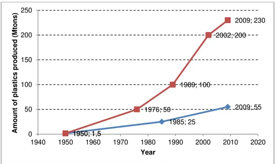
Figure 1.1 - World (red line and symbols) and Europe (blue line and symbols) plastics production between 1950 and 2009 [source: Plastics Europe Market Research Group (PEMR), from (Association of Plastics Manufacturers in Europe (APME) 2010)]. ... 3
Figure 1.2 - World plastics production in 2009 [source: PlasticsEurope Market Research Group (PEMR), from (Association of Plastics Manufacturers in Europe (APME) 2010)]. ... 4
Figure 1.3 - Europe (EU27, Norway and Switzerland) plastics demand by polymer types in 2009 [source: PlasticsEurope Market Research Group (PEMRG), from (Association of Plastics Manufacturers in Europe (APME) 2010)]. ... 5
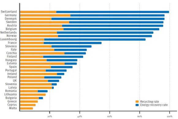
Figure 1.4 - Total recovery ratio by country (referred to post-consumer plastic waste), in 2009 [source: (Association of Plastics Manufacturers in Europe (APME) 2010)]. ... 6
Figure 1.5 - llustration of the initiation step according to a free radical chain mechanism for PE thermal degradation [adapted from (Bockhorn, Hornung et al. 1999)]. ... 8
Figure 1.6 – Possible paths that allows the β-scission of the more radicals, resulting a primary radical and an olefin [adapted from (Bockhorn, Hornung et al. 1999)]. ... 9
Figure 1.7 - Intramolecular –hydrogen- transfer- formation of a more stable radical from a primary one [adapted from (Bockhorn, Hornung et al. 1999)] ... 9
Figure 1.8 - Formation of more stable radicals, via intermolecular hydrogen transfer [adapted from (Bockhorn, Hornung et al. 1999)]. ... 9
Figure 1.9 – Termination step according to a free radical chain mechanism (adapted from (Bockhorn, Hornung et al. 1999)). ... 10
Figure 1.10 - Illustration of the general process of plastics catalytic degradation [adapted from (Contreras, Garcia et al. 2012)]. ... 11
xv Figure 1.12 – Initiation step of PE catalytic cracking by means of an olefin protonation by a Brönsted
acid site... 13
Figure 1.13 - Initiation step of PE catalytic cracking by means of Lewis acid site hydride-ion abstraction. ... 13
Figure 1.14 - Isomerization step according to carbocation mechanism of PE’s catalytic cracking [adapted from (Buekens, Huang 1998)]. ... 14
Figure 1.15 - Formation of an olefinic carbenium ion that undergoes further cyclization, according to carbocation mechanism of PE’s catalytic cracking [adapted from (Buekens, Huang 1998)]. ... 14
Figure 1.16 - Formation of aromatics by means of an intramolecular attack on the double bond in a olefinic carbenium ion that undergoes further cyclization, according to carbocation mechanism of PE’s catalytic cracking [adapted from (Buekens, Huang 1998)]. ... 15
Figure 1.17 - Haag-Dessau cracking mechanism for an alkane molecule (RH) proceeding by means of carbonium ion [adapted from (Kotrel, Knözinger et al. 2000) ] ... 15
Figure 1.18 - Preferential protonation and collapse of a 3-methylpentane molecule [adapted from (Kotrel, Knözinger et al. 2000)] ... 16
Figure 2.1 – Temperature profile for vaporization of pure hydrocarbons kinetics experiments. ... 23
Figure 2.2 - Temperature profile for vaporization of hydrocarbons mixtures kinetics experiments. ... 23
Figure 2.3 - Temperature profile for thermal and catalytic degradation of polyethylene experiments. . 23
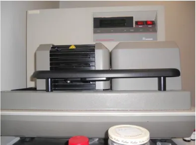
Figure 2.4 – DSC/TG installation used in the experiments performed: a) balance; b) furnace; c) gas (N2) flow controller; d) computer; e) gas (N2) line). ... 24
Figure 2.5 – TG/DSC instrument (TA Instruments ® SDT 2960). ... 24
Figure 2.6 – Gas (N2) flow measurer. ... 25
Figure 2.7 – Two pans suspended in the balance’s arms with the oven open. ... 25
xvi
Figure 3.2 - Simplified flowchart for the computational model. ... 29
Figure 3.3 – Sequence of computations in a cycle: a) initial state b) all bonds are scanned and decision on which are broken is made; c) bond array is scanned again to identify molecules that were formed and d) decision on evaporation is made. ... 30
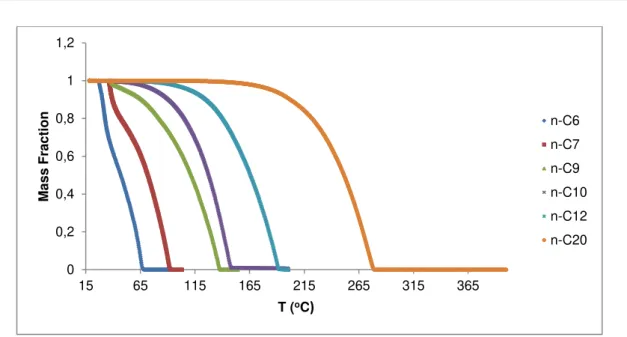
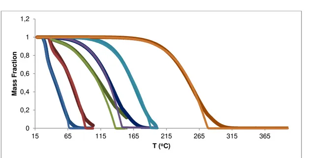
Figure 4.1 –Vaporization curves for the hydrocarbons studied, obtained from TG/DSC results. ... 32
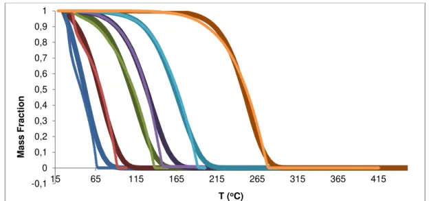
Figure 4.2 – Experimental (symbols) and individual fitting vaporization curves (lines): n-hexane (blue), n-heptane (red), n-nonane (green), n-decane (violet), n-dodecane (light blue) and n-icosane (orange). ... 35
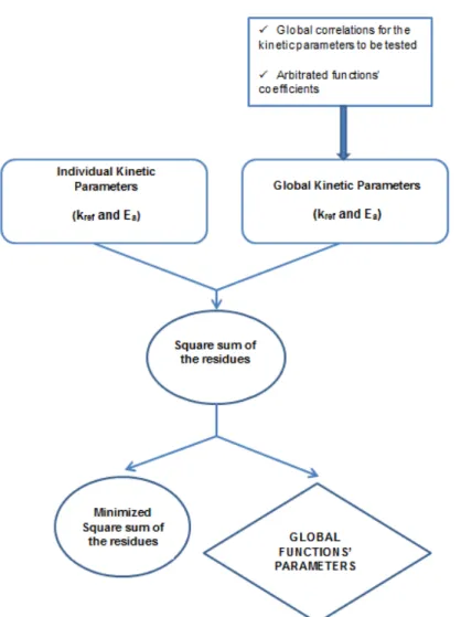
Figure 4.3 – Flowchart that illustrates the method I for obtaining the global correlations’ coefficients. 37
Figure 4.4 - Flowchart that illustrates the method II for obtaining the global correlations’ coefficients 38
Figure 4.5 – Experimental and simulated [kref exponential; Ea quadratic; method I) vaporization curves, respectively, for: n-hexane (blue dots and line); n-heptane (red dots and line); n-nonane (green dots and line); n-decane (violet dots and line); n-dodecane (light blue dots and line) and n –icosane (orange dots and line)]. ... 40
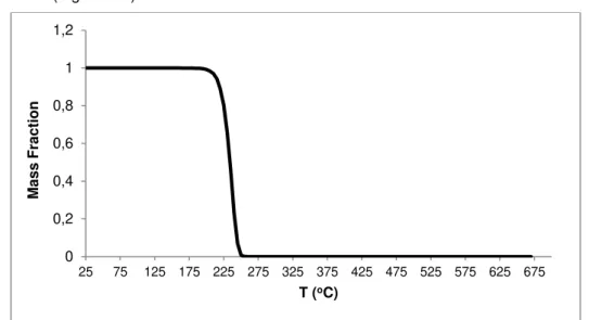
Figure 4.6 – Rate of vaporization for n-C40, simulated by the computational model (quadratic function for Ea, exponential function for kref; method I) ... 41
Figure 4.7 – kinetic parameters’ values for the different paraffins: krefv from individual fitting (blue symbols) and from global fitting (blue line) and Eav from individual fitting (red symbols) and from global fitting (red line); global laws: quadratic for Ea and exponential for kref, method II. ... 42
Figure 4.8 - Experimental and simulated [krefv exponential; Eav quadratic; method II) vaporization curves, respectively, for: n-hexane (blue dots and line); n-heptane (red dots and line); n-nonane (green dots and line); n-decane (violet dots and line); n-dodecane (light blue dots and line) and n – icosane (orange dots and line)]. ... 43
xvii Figure 4.10- Rate of vaporization for n-C40, simulated by the computational model (3rd degree polynomial function for Eav, exponential function for krefv; method I) ... 46
Figure 4.11 - Experimental rates of vaporization and simulated [krefv exponential; Eav linear; method I) vaporization curves, respectively, for: hexane (blue dots and line); heptane (red dots and line); n-nonane (green dots and line); n-decane (violet dots and line); n-dodecane (light blue dots and line) and n –icosane (orange dots and line)]. ... 48
Figure 4.12 - Kinetic parameters’ values for the different paraffins: krefv from individual fitting (blue symbols) and from global fitting (blue line) and Eav from individual fitting (red symbols) and from global fitting (red line); global laws: linear for Eav and exponential for krefv, method II. ... 49
Figure 4.13 - Experimental rates of vaporization and simulated [krefv exponential; Eav linear; method II) vaporization curves, respectively, for: hexane (blue dots and line); heptane (red dots and line); n-nonane (green dots and line); n-decane (violet dots and line); n-dodecane (light blue dots and line) and n –icosane (orange dots and line)]. ... 50
Figure 4.14 -Experimental rates of vaporization and simulated [krefv exponential; Eav function defined by segments; method I) vaporization curves, respectively, for: n-hexane (blue dots and line); n-heptane (red dots and line); n-nonane (green dots and line); n-decane (violet dots and line); n-dodecane (light blue dots and line) and n –icosane (orange dots and line)]. ... 52
Figure 4.15 - kinetic parameters’ values for the different paraffins: krefv from individual fitting (blue symbols) and from global fitting (blue line) and Eav from individual fitting (red symbols) and from global fitting (red line); global laws: function defined by segments for Eav and exponential for krefv, method II. ... 53
Figure 4.16 - Experimental rates of vaporization and simulated [kref exponential; Ea function defined by parts; method II) vaporization curves, respectively, for: n-hexane (blue dots and line); n-heptane (red dots and line); n-nonane (green dots and line); n-decane (violet dots and line); n-dodecane (light blue dots and line) and n –icosane (orange dots and line)]. ... 54
Figure 4.17 - experimental and modeled vaporization curves, respectively, for: n-decane [blue dots and line); n-dodecane (red dots and line); n-decane + n-dodecane (green dots and line)]. ... 58
xviii
Figure 5.1 - a): HDPE thermal degradation curves: experimental (blue dots), assay nr. 1 (red line), assay nr. 2 (green line) and assay nr. 3 (orange line); b) DSC signals: experimental (blue dots), assay nr. 1 (red line), assay nr. 2 (green line) and assay nr. 3 (orange line); c) HDPE thermal degradation curves: experimental (blue dots), assay nr. 4 (red line), assay nr. 5 (green line) and assay nr. 6 (orange line); d) DSC signals: experimental (blue dots), assay nr. 4 (red line), assay nr. 5 (green line) and assay nr. 6 (orange line); e) HDPE thermal degradation curves: experimental (blue dots), assay nr. 7 (red line), assay nr. 8 (green line) and assay nr. 9 (orange line); f) DSC signals: experimental (blue dots), assay nr. 7 (red line), assay nr. 8 (green line) and assay nr. 9 (orange line) ... 64
Figure 5.2 - Blue symbols: values of ln(k) vs (1/T) for the thermal degradation of HDPE with kref= 2x10 -5 min-1 and E
a = 20000 cal/mol; red symbols: values of ln(k) vs (1/T) for the thermal degradation of HDPE with kref= 2x10⁻⁵ min-1 and Ea = 40000 cal/mol; vertical dashed line: represents the fixed
reference temperature (300 K 1/T ≈ 0,0033 K-1). ... 66
Figure 5.3 - HDPE catalytic degradation curves: experimental (blue dots), assay nr. 1 (red line), assay nr. 2 (green line) and assay nr. 3 (orange line); b) DSC signals: experimental (blue dots), assay nr. 1 (red line), assay nr. 2 (green line) and assay nr. (orange line); c) HDPE catalytic degradation curves: experimental (blue dots), assay nr. 4 (red line), assay nr. 5 (green line) and assay nr. 6 (orange line); d) DSC signals: experimental (blue dots), assay nr. 4 (red line), assay nr. 5 (green line) and assay nr. 6 (orange line); e) HDPE catalytic degradation curves: experimental (blue dots), assay nr. 7 (red line), assay nr. 8 (green line) and assay nr. 9 (orange line); f) DSC signals: experimental (blue dots), assay nr. 7 (red line), assay nr. 8 (green line) and assay nr. 9 (orange line). .... Erro! Marcador não definido.
Figure 5.4 - Best fitting obtained using the stochastic model for thermal degradation of HDPE [kref = 2 x 10⁻⁵ min-1 and Ea = 30 000 cal.mol-1): a) experimental TG curve (blue dots) and simulated TG curve (green line); b) experimental DSC curve (blue dots) and simulated DSC curve (green line)]. ... 70
Figure 5.5 - Best fitting obtained using the stochastic model for catalytic degradation of HDPE [kref = 1 x 10⁻³ min-1 and Ea = 20 000 cal.mol-1): a) experimental TG curve (blue dots) and simulated TG curve (orange line); b) experimental DSC curve (blue dots) and simulated DSC curve (orange line)]. ... 70
Figure 5.6 – best fitting provided by the stochastic model developed for HDPE thermal degradation: a) TG experimental (blue dots) and simulated (red line) curves; b) DSC experimental (blue dots) and simulated (red line) curves. ... 72
xix Figure 6.1 –PC SPARTAN PRO 6 software commands to calculate an equilibrium geometry. ... 78
Figure 6.2 – Molecular models used in the software that represent the regents from all scission reactions (green spheres: chloride atoms; dark grey sphere in acidic sire representation: silicon atom; red sphere: oxygen atom; dark grey spheres: carbon atoms; white spheres: hydrogen atoms). ... 79
Figure 6.3 – Molecular model of a transition-state complex associated to the scission of the bond in position 5 (illustrates the action of constraining bonds). ... 79
Figure 6.4 – Commands used in PC SPARTAN PRO 6 software to perform an equilibrium geometry
optimization subjected constraints and additional IV spectrum request. ... 80
Figure 6.5 – How to display a IV spectrum in PC SPARTAN PRO 6 software. ... 80
Figure 6.6 – Illustration of a single-negative frequency in a IV spectrum. ... 80
Figure 6.7 – Commands used in PC SPARTAN 6 ® software to optimize a transition state-geometry,
including an IV spectrum request. ... 81
Figure 6.8 – Output data from a molecular simulation. ... 82
Figure 6.9 – Distribution of the activation energy calculated with base on PC SPARTAN 6 ® software
xx
L
IST OF
T
ABLES
Table 2.1 - List of the materials used in this work experiments as well as in the assays performed in previous works whose data are used (VKPH- vaporization of pure hydrocarbons kinetics; VKHM – vaporization of hydrocarbons mixtures’ kinetics; TCDPE – thermal and catalytic degradation of HDPE; n.a. – not applicable). ... 21
Table 2.2 – Composition of the hydrocarbons mixtures used. ... 22
Table 4.1 – Approximated temperatures of vaporization for the paraffins in study. ... 32
Table 4.2 - Kinetic parameters obtained by the individual fitting, approximate temperatures of vaporization estimated from fitted curves and sum of the residues minimized by the “Solver” tool. .... 35
Table 4.3 – Simulation conditions used for all simulations performed in vaporization kinetic of pure hydroacarbon studies (Ti– initial simulation temperature; Tf– final simulation temperature; β– heating rate; dt – integration step; Cp – average heat capacity; ΔH(C-C) – average C-C bond enthalpy; kref – cracking kinetic constant rate at reference constant; ΔHvap – average vaporization enthalpy; nr. Molecules – number of molecules used in the simulation). ... 39
Table 4.4 - Global fitting results (exponential function for krefv; quadratic function for Eav; method I). .. 40
Table 4.5 - global fitting results (exponential function for krefv; quadratic function for Eav; method II). .. 41
Table 4.6 - Global fitting results (exponential function for kref; 3rd degree polynomial function for Ea; method I). ... 44
Table 4.7 - Global fitting results (exponential function for krefv 3rd degree polynomial function for Eav; method II). ... 46
Table 4.8 - Global fitting results (exponential function for kref; linear function for Ea; method I). ... 47
Table 4.9 - Global fitting results (exponential function for kref; linear function for Ea; method II). ... 48
Table 4.10 - Global fitting results (exponential function for kref; function defined by parts for Ea; method
xxi Table 4.11 global fitting results (exponential function for kref; function defined by parts for Ea; method
II) ... 53
Table 4.12 - simulation charecteristics summary ... 55
Table 5.1 - simulation conditions used for all simulations performed in thermal and catalytic degradation of HDPE studies (Ti– initial simulation temperature; Tf– final simulation temperature; β– heating rate; dt – integration step; Cp – average heat capacity; ΔH(C-C) – average C-C bond enthalpy; k
– cracking kinetic constant rate; ΔHvap – average vaporization enthalpy; nr. bonds – number of bonds per molecule; nr. molecules – number of molecules used in the simulation). ... 62
Table 5.2 – values of the kinetic parameters used for thermal degradation of PE simulations. ... 63
Table 5.3 – values of the kinetic parameters used in each simulation performed in thermal degradation of PE. ... 63
Table 5.4 – Effect of the kinetic parameters variation on TG simulated curves for PE thermal degradation. ... 65
Table 5.5 - - Effect of the kinetic parameters variation on DSC simulation signals for PE thermal degradation. ... 65
Table 5.6 - Values of the kinetic parameters used for catalytic degradation of PE simulations ... 67
Table 5.7 - Values of the kinetic parameters used in each simulation performed in catalytic degradation of PE. ... 67
Table 5.8 - simulation conditions used for the best fitting performed for the thermal degradation of HDPE (Ti – initial simulation temperature; Tf – final simulation temperature; β – heating rate; dt – integration step; Cp – average heat capacity; ΔH(C-C) – average C-C bond enthalpy; kref – cracking kinetic constant rate at reference temperature; ΔHvap – average vaporization enthalpy; nr. bonds – number of bonds per molecule; nr. molecules – number of molecules used in the simulation). ... 72
xxii
Table 6.1 – performance and cost of some models existing in PC SPARTAN PRO 6 ® software
[adapted from (Hehre, Yu et al. 1998)]. ... 77
Table 6.2 – relation between the bond- chain position where scission occurs and the products formed, for all molecular simulations carried out. ... 82
Table 6.3 – activation energy values calculated with base on PC SPARTAN 6 ® software for the
xxiii
N
OMENCLATURE
APME Association of Plastics Manufacturers in Europe % (w/w) Mass percentage
∆H(C-C) Average C-C bond enthalpy
∆Hvap Average vaporization enthalpy
Cp Average Heat Capacity
DSC Differential Scanning Calorimetry
DSC/TG simultaneous Differential Scanning Calorimetry and Thermogravimetry dt Time step of integration
Ea Activation energy of the cracking process Eav Activation energy of vaporization
FCC Fluid Catalytic Cracking GC Gas Chromatography
GC-MS Gas Chromatography – Mass Spectrometry h Plank's constant
HDPE High-density Polyethylene
k(T) Temperature-dependent cracking kinetic constant rate kref Crackingkinetic constant rate at reference temperature krefv Vaporizationkinetic constant rate at reference temperature kv (T) Temperature-dependent kinetic constant rate of vaporization LDPE Low-density Polyethylene
LLDE Linear Low-density Polyethylene m Experimental weight of the sample m mod mixt (t)
Total weight of the sample given by the model (vaporization of hydrocarbon's mixtures)
m total sample Totalweight of the sample
m0 mixt Initial sample of the hydrocarbon's mixture sample
me Electron mass
mh Weight of the heavier hydrocarbon in the mixture mheat Mass of bonds heated per time unit
ml Weight of the lighter hydrocarbon in the mixture MSW Municipal solid wastes
mv Mass of bonds evaporated per time unit nb Number of bonds broken per time unit
n-C6 n-hexane
n-C7 n-heptane
n-C9 n –nonane
n-C10 n-dodecane
n-C12 n-dodecane
n-C20 n-icosane
xxiv
Nr. Molecules Number of molecules PE Polyethylene
PET Polyethylene therephtalate PP Polypropylene
PVC Polyvinyl chloride
px Probability of the occurrence of the first-order processes of vaporization and cracking r Distance between the nuclear and the electron charges
T Temperature
t Time
TCDPE Thermal and Catalytic Degradation of Polyethylene Tf Final temperature used in the simulation process TG Thermogravimetry
TGA Thermogravimetric Analysis
Ti Initial temperature used in the simulation process Tref Reference Temperature
Tvaporization Approximated vaporization temperature
VMHK Vaporization of Mixtures of Hydrocarbons Kinetics VPHK Vaporization of Pure Hydrocarbon Kinetics
X Mass fraction
X mod Mass fraction obtained from m mod mixt (t) and m0 mixt
Xexp Mass fraction associated to experimental data Xglob Mass fraction by means of the global fitting
Xind Mass fraction obtained by means of the individual fittings
Z Atomic charge
α Number of bonds lost to the gas phase
β Heating rate
1
M
OTIVATION AND
M
AIN
O
BJECTIVES
In the last years, a huge amount of plastics has been produced as result of their versatility of applications and low cost production. Among the various types of plastics produced, polyethylene is the one which is majorly consumed. This massive plastic production leads to a social and environmental issue related to waste management, since the residues have low biodegradability and high chemical inertness. Therefore, an increasingly amount of municipal solid waste in landfills has been observed.
Thus it is urgent to develop techniques that allow, at the same time, the proper disposal of the wastes and to harness of the plastic residues potential.
In the case of polyethylene, its catalytic degradation emerges as an efficient alternative to achieve that goal. With this process, it is possible to eliminate PE waste and convert it into added value hydrocarbons that can be used as chemicals or fuels. This latter aspect makes the process even more advantageous due to petroleum resources scarcity.
For such an important technique in terms of energetic, social and environmental issues, it is crucial to have a deeper knowledge for a possible further industrial implementation. For this purpose, the modeling of the process emerges as a powerful tool since it allows predicting the reaction process. Starting from this background, the main goal of this work is to contribute to the development of a reliable model that can predict the thermal and catalytic degradation of polyethylene.
The most used technique to evaluate this reaction is the simultaneous DSC/TG analysis. The models that are already developed to predict the latter process are deterministic ones and present a major limitation since they do not work in an autonomous way, i.e., they can predict thermal and catalytic of PE but only partially or using experimental information.
The objective of this work is to develop a stochastic model that allows the prediction of the process in a reliable ab initio way, only by inserting the operation conditions, thermodynamic and
kinetic data, as well as the type and number of molecules whose degradation is tested. Therefore, the drawbacks of the deterministic models can be solved.
3
1. I
NTRODUCTION
1.1.
Plastic materials demand and production
If we take a look to our day-to-day lives, it is easy to identify a countless number of objects made of plastic and it is also easy to understand our huge dependence on this type of materials. In fact, due to an enormous growth of welfare in the second half of the twentieth century and simultaneously due to plastic’s excellent properties and low cost, we have witnessed a huge increase in their demand and, consequently, in their production in the last decades, unparalleled in other materials (Gobin, Manos 2004, Contreras, Garcia et al. 2012)
According to a 2010 report from Association of Plastics Manufacturers in Europe (Association of Plastics Manufacturers in Europe (APME) 2010), the world plastics industry has grown continuously in the last fifty years, being verified an increase in the production from 1,5 million tons in 1950 to 230 million tons in 2009, which corresponds to an increment of 9% per year, on average (see Figure 1.1).
Figure 1.1 - World (red line and symbols) and Europe (blue line and symbols) plastics production between
1950 and 2009 [source: Plastics Europe Market Research Group (PEMR), from (Association of Plastics
Manufacturers in Europe (APME) 2010)].
In the same study (Association of Plastics Manufacturers in Europe (APME) 2010) it is also noticeable that in 2009, from the 230 million tons of the plastics produced in the world, around 24% were manufactured in the European continent (comprises EU27, Norway and Switzerland) in a total of 55 million tons.
1950; 1,5 1985; 25 2009; 55 1950; 1,5 1976; 50 1989; 100 2002; 200 2009; 230 0 50 100 150 200 250
1940 1950 1960 1970 1980 1990 2000 2010 2020
4
Figure 1.2 - World plastics production in 2009 [source: PlasticsEurope Market Research Group (PEMR),
from (Association of Plastics Manufacturers in Europe (APME) 2010)].
Among the amount of polymers produced in Europe, in 2009, there are five high-volume plastics families: polyethylene (PE), polypropylene (PP), polyvinyl chloride (PVC), polystyrene (solid PS and expandable PS) and polyethylene terephtalate (PET). In fact, these five types of polymers account for around 75% of all European plastics demand (see Figure 1.3).
5
Figure 1.3 - Europe (EU27, Norway and Switzerland) plastics demand by polymer types in 2009 [source:
PlasticsEurope Market Research Group (PEMRG), from (Association of Plastics Manufacturers in Europe
(APME) 2010)].
1.2.
Plastic wastes: is it possible to have a life after consumption?
As it is shown in Figure 1.2 and Figure 1.3, millions of tons of plastics are produced every year. This massive consumption leads to a proportional emergence in the amount of plastic residues since a lot of the applications correspond to low lifetime products. To get an idea of this huge phenomenon, in the last decade the consumption of plastics has led to a consequent 3% increment in post-consumer end-of-life plastic waste (Association of Plastics Manufacturers in Europe (APME) 2010) Moreover, in Europe, in 2004, the 40 millions of plastic material consumed have been transformed into 30 million tons of waste. As it is known, the low biodegradability and chemical inertness of such materials make their wastes’ disposal a serious environmental problem (Contreras, Garcia et al. 2012).
The most current methods to manage municipal solid wastes (MSW), where plastic residues are included, are landfill and incineration (Coelho 2008).
In the first disposal method, there’s a problem relating with the fact that plastics take a considerable time to break down at landfills (Coelho 2008). Thus, they occupy a large volume of landfills sites or rubbish tips, which is exacerbated by the fact that this waste type is more voluminous than others, leading to scarcity of disposal areas (Association of Plastics Manufacturers in Europe (APME) 2010, Gobin, Manos 2004, Contreras, Garcia et al. 2012, Coelho 2008) Additional drawbacks are associated to this disposal technique: the process generates explosive and toxic gases and its costs are become higher and higher (Association of Plastics Manufacturers in Europe (APME) 2010, Contreras, Garcia et al. 2012, Coelho 2008)
6
al. 2012). Nonetheless, because of the generation of toxic gases, it can be said that this process shifts a solid waste issue to an air pollution one (Gobin, Manos 2004). Moreover, the high operating temperatures, the fact that the energy released is often not properly harnessed and due to the production of compounds with a very low economic value, this method is criticized by several environmentalists and researchers.(Contreras, Garcia et al. 2012).
By means of the previous methods it is not possible to take advantage of the whole plastic waste potential and there are also environmental issues associated, which make them unreliable treatments. Therefore, to take full advantage of these residues, part of the solution has to be the acceptance by society to use resources efficiently and that these valuable materials should not go to landfill or direct incineration. In this way, restrictions on landfilling are being implemented through countries legislation (Association of Plastics Manufacturers in Europe (APME) 2010). These restrictions create strong drivers to increase both recycling and energy recovery which has taken rates above 80% in 2009, according to (Association of Plastics Manufacturers in Europe (APME) 2010). In fact, plastic wastes’ re-use, due to their high content of carbon and calorific value, allows their using as a raw material or as fuel source, making them an available supply of chemicals and energy (Coelho, Costa et al. 2010). As it can be observed in Figure 1.4, this process of capture value from plastic (from recycling and energy recovery) waste is underway, even though it is slow: there’s an increase of only 2% per year (Association of Plastics Manufacturers in Europe (APME) 2010).
Figure 1.4 - Total recovery ratio by country (referred to post-consumer plastic waste), in 2009 [source:
7 Thus it can be concluded that plastic materials can have a “life” after their consumption but only if recycling methods are used to treat them. Indeed, one can say: “plastics are too valuable to throw away!” (Association of Plastics Manufacturers in Europe (APME) 2010).
A recycling method is now presented. Even though it has still handicaps, mechanical recycling presents some features that provide taking advantage of plastic waste value.
According to (Association of Plastics Manufacturers in Europe (APME) 2010), the EU members plus Norway and Switzerland, in 2009, from the 24,3 million of tons of post-consumer waste produced, have treated 22,2% through mechanical recycling. It comprises a way to reprocess the end-of-plastics into re-usable materials through a physical treatment that doesn’t break the original polymer chains and molecules, leaving material’s original structure and properties intact (Association of Plastics Manufacturers in Europe (APME) 2010).
This technique include the steps of sorting the polymeric residues by type, shredding the waste into particles of smaller dimensions, melting them down and remolding the thermoplastic to transform it into new-machine ready granules (Association of Plastics Manufacturers in Europe (APME) 2010, Contreras, Garcia et al. 2012).
Unlike landfilling and incineration, the recycled materials obtained with the current method are welcomed by society. Nevertheless, there are some drawbacks associated with it: the products have a very poor quality since the residues are subjected to high temperatures melting and also due to the varying quality of the original waste and the eventual presence of impurities and additives (Contreras, Garcia et al. 2012). Besides the recycled products are often more expensive than the virgin material (Garforth, Ali et al. 2005).
1.3.
Plastic waste pyrolysis or degradation
As a way to harness the whole potential of plastic waste a different technology based on polymer pyrolysis has appeared; this allows the transformation of these residues into high added value hydrocarbons (liquid or gaseous) to be used as chemicals and/or fuel (Contreras, Garcia et al. 2012, Coelho, Costa et al. 2012) . For these reasons, the present technique becomes a good alternative to the methods already outlined (Gobin, Manos 2004, Contreras, Garcia et al. 2012, Coelho, Costa et al. 2012) since it solves the disposal problems and spares the petroleum resources (Coelho, Costa et al. 2012)
8
Thermal degradation of polyethylene
1.3.1.
General considerations
a.
The thermal degradation of polyethylene presents some advantages when compared to the other methods of polymeric waste management that have already been showed.
Nevertheless, pure thermal degradation requires high operation temperatures, ranging from 500oC to 800oC (Contreras, Garcia et al. 2012). In fact, according to (Coelho, Costa et al. 2012), the degradation temperature of HDPE in a purely thermal assay under dynamic conditions in an inert atmosphere is around 483oC. These operation conditions and the fact that the cracking reactions are endothermic require, consequently, a high energetic input (Contreras, Garcia et al. 2012, Gobin, Manos 2004). Due to the factors enunciated before, together with the production of poor quality compounds, the current recycling method became economically unattractive (Gobin, Manos 2004, Coelho, Fonseca et al. 2010, Coelho, Costa et al. 2012, Contreras, Garcia et al. 2012).
Reaction mechanism
b.
There are four types of reaction mechanisms associated with the thermal cracking of plastics: end-up chain scission; random-chain scission; chain-stripping or cross-linking (Buekens, Huang 1998). The different mechanisms and, consequently, the product distributions are related with bond dissociation energies, chain defects in the polymers, the aromaticity degree, as well as the presence of hetero-atoms in the polymer-chain (Buekens, Huang 1998). PE pyrolysis, in turn, occurs through a random-chain scission mechanism (Scoethers, Buekens 1979) that will be outlined in the following paragraphs.
When a certain amount of heat supplied to a long chain of ethylene monomers, the scission of the polymer bonds occurs and smaller fragments are produced (Coelho 2008). Since all C-C bonds in the polymer chain have, in principle, the same strength, bond scission is expected to occur randomly (Coelho 2008).
According to (Bockhorn, Hornung et al. 1999), the general mechanism for thermal degradation of polyethylene can be described as follows:
Due to the heat applied, the degradation reaction is initiated by an homolytic random scission of the polymer chain into primary radicals (species with an unpaired electron). This step is called initiation (see Figure 1.5);
Figure 1.5 - llustration of the initiation step according to a free radical chain mechanism for PE thermal
9 Following initiation, a propagation step takes place. It can occur by means of two different
ways1: intramolecular hydrogen transfer or intermolecular hydrogen transfer;
Intramolecular hydrogen transfer is favored by lower temperatures and it consists in two stages: first there is a hydrogen transfer within the primary radical molecule. Thus is obtained a more stable radical (e.g. secondary, tertiary, etc.) (see Figure 1.6). This new stable radical undergoes a new reaction stage and, by means of β-scission, origins a primary radical and an olefin, according to two different paths. The primary radicals will continue the depolymerization;
At higher temperatures, the abstraction of a hydrogen atom by means of intermolecular hydrogen transfer between a primary radical and a paraffin fragment, to form a paraffin and a more stable radical occurs (see Figure 1.8);
1
Note that these two paths of the depolymerization occur simultaneously, even though their extension is controlled thermodynamically, namely by the influence of temperature.
Figure 1.6 – Possible paths that allows the β-scission of the more radicals, resulting a primary radical and
an olefin [adapted from (Bockhorn, Hornung et al. 1999)].
Figure 1.7 - Intramolecular –hydrogen- transfer- formation of a more stable radical from a primary one
[adapted from (Bockhorn, Hornung et al. 1999)]
Figure 1.8 - Formation of more stable radicals, via intermolecular hydrogen transfer [adapted from
10
Finally, termination steps occur by combination of two primary radicals to form an inert molecule (see Figure 1.9).
Figure 1.9 – Termination step according to a free radical chain mechanism (adapted from (Bockhorn,
Hornung et al. 1999)).
Promising improvements
c.
As it was seen previously, although this process presents some advantages in relation to mechanical recycling and, in turn, to landfill and incineration (Association of Plastics Manufacturers in Europe (APME) 2010), there are still some drawbacks associated to its operation conditions and product’s quality.
More recently, it has been proved that the use of solid catalysts presents as a promising technique (Association of Plastics Manufacturers in Europe (APME) 2010, Contreras, Garcia et al. 2012, Gobin, Manos 2004, Coelho, Fonseca et al. 2010, Coelho, Costa et al. 2012, Marcilla, Gómez-Siurana et al. 2007, Marcilla, Gómez-Gómez-Siurana et al. 2007).
In the following subchapter this alternative process, the catalytic degradation of polyethylene, will be more minutely outlined.
Catalytic degradation of polyethylene
1.3.2.
General considerations
a.
In order to improve the thermal degradation of polyethylene and solve some of the problems associated with its valorization, the use of solid catalysts seems to be a promising alternative. In a general way, the use of catalysts allows the reduction of process temperature, resulting in a reduction of the energetic input, as well as it makes possible to control hydrocarbons product distribution. In this way, hydrocarbons products in the motor fuel boiling point range are formed, which means that materials of high added value are obtained and their upgrade is no longer necessary (Association of Plastics Manufacturers in Europe (APME) 2010, Contreras, Garcia et al. 2012, Gobin, Manos 2004, Coelho, Fonseca et al. 2010, Coelho, Costa et al. 2012). These products are those which are suitable for liquid fuel usage. In fact, when compared to thermal cracking, this process produces more volatile hydrocarbons2 such as those in the range of C
5-C9 and compounds with a greater octane index3, such as aromatics, naphtenes and iso-alkanes (in the previous mentioned range) (Buekens, Huang 1998).
2
11 These improvements make the process economically viable (Marcilla, Gómez-Siurana et al. 2007, Gobin, Manos 2004, Contreras, Garcia et al. 2012, Coelho, Fonseca et al. 2010, Coelho, Costa et al. 2012).
In a general way, this process can be schematized as follows (Figure 1.10):
Figure 1.10 - Illustration of the general process of plastics catalytic degradation [adapted from (Contreras,
Garcia et al. 2012)].
Most used catalysts
b.
The most commonly used catalysts are porous solid catalysts such as mesoporous and microporous materials like MCM-41, pillared clays and different zeolites (HY, H-ZSM-5, H-Beta), being the last ones the most studied catalysts (Coelho 2008, Contreras, Garcia et al. 2012, Gobin, Manos 2004, Marcilla, Gómez-Siurana et al. 2007).
According to (García, Serrano et al. 2005), there’s a direct correlation between catalysts’ acidity and pore size with the compounds produced by cracking. In one hand, the cracking of polyethylene using mesoporous catalysts like MCM-41, due to its large pore size and medium acidity, produces hydrocarbons within the range of gasoline, which may be explained from the occurrence of a random scission mechanism. On the other hand, ZSM-5 catalyzed degradation of PE results in the formation of lighter and gaseous hydrocarbons and some aromatic compounds. This product distribution is achieved due, for example, to and an end-chain cracking mechanism which is consequence of its small pore size and strong acidity (García, Serrano et al. 2005).
Like catalysts’ acidity and pore size, the particle size also plays an important role on the production of the degradation products type. Both for H-ZSM-5 and H-Beta zeolites, showed a high cracking activity due to their large external surface area and low diffusional problems. On contrary, amorphous silica-alumina MCM-41 showed lower values of activity (García, Serrano et al. 2005).
H-ZSM-5 and HY zeolite catalysts are used in the fluid catalytic cracker (FCC) and can in fact degrade PE with a higher yield on hydrocarbons and obtain a relatively low coke content ( <1% (w/w) and 8% (w/w), respectively), confirming, thus, the possibility of co-fed a refinery cracking unity with plastic waste.
12
)
)
Zeolite catalysts fundamentals
4c.
Zeolite catalysts are crystalline materials and are part of a family of materials denominated aluminosilicates. Their structure is based on a tridimensional framework of tetrahedrical sites TO4 (SiO4 or AlO4-) linked by the oxygen atoms. The repetition of these unities leads to a microporous structure that can consist of channels and/or cavities.
Due to the existence of trivalent aluminium atoms, the overall zeolite framework has a negative charge which is compensated by the existing cations (usually metals or protons) in the lattice, ensuring, in this way, the electrical neutrality.
The ability to modify, in an easy way, the composition, structure and porosity of these compounds, either by direct synthesis or by post-synthesis treatments (dealumination, ion exchange, etc) have led researchers to produce more than 130 different types of zeolites. Therefore, zeolites can be used in acid, basic, acid-base, redox or bifunctional catalysis, even though they are mostly used in acid and bifunctional catalysis. In catalytic degradation of polyethylene by using zeolites, acid catalysis is used.
In zeolites there are two types of acid sites: Brønsetd acid sites and Lewis acid sites.
Brønsetd acid sites are related with the presence of hydroxyl (OH) groups. These in turn can be
classified in: structural or bridging groups [SiO(H)Al], terminal silanol groups [SiOH] and aluminium hydroxyl groups [AlOH]. The first type of OH groups represents Brønsetd acid sites which are the
strongest and are located mainly in the zeolites microporous. On the other, terminal silanol groups are usually generated in the external surface of zeolite’s structure or by the presence of structural defects. Finally, the last type of acid sites result from the existence of an aluminium extra-framework phase.
Lewis acid sites are electron acceptors sites and, thus, are not related to the presence of hydroxyl group. Instead, they are associated with the tri-coordinate aluminium and another cationic species present.
An important information on zeolite’s acidity is the silicon to aluminium ratio (or silica to alumina – SiO2/Al2O3 ratio), which is related to the number of acid Brønsetd sites. In fact, the total number of
4 This subchapter is based on the following reference: (Guisnet, Ramôa 2004)
Figure 1.11 – Chemical structure of a zeolite [adapted from (Haag, Lago et al. 1984) ] (on reader’s left
13 such acid sites corresponds to the number of tetrahedral aluminium atoms in the framework, which are balanced by the presence of protons to ensure the electrical neutrality. An increasing in Si/Al value means that the number of Brønsetd sites decreases since the fraction of Al atoms also decreases. On
the other hand, decreasing the Si/Al ratio also causes an increment in Brønsetd acid sites strength.
A way to increase Lewis acidity is the presence of multivalent cations in the zeolite lattice.
Reaction mechanism
d.
The cracking occurred in FCC unities in refinery can be explained with basis in a carbocation reaction mechanism due to the acidity of the catalysts’ Lewis or Brønsted sites (Buekens, Huang
1998). For catalytic cracking of polyethylene, similar mechanisms have been postulated (Buekens, Huang 1998). It is now accepted that catalytic cracking occurs through the formation of carbocations and two mechanisms are possible: by formation of carbenium ions (paraffin with a carbon atom tri-coordinated and positively charged) or by formation of carbonium ions (paraffins with a carbon atom penta-coordinated, positively charged) (Rebelo 2009).
Carbenium-ion mechanism
I. Initiation step
There are two possible ways of initiation step to occur: by protonation of an olefinic bond by a Brönsted acid site or by the hydride abstraction in Lewis acid sites.
The initiation possibility concerning the protonation of a double bond may be related to the existence of defect sites in polymer’s chain (e.g. an olefinic bond). On these olefinic defects, the Brønsted acid sites from the acid catalyst, HX, attack, by proton addition, being produced a carbenium
ion and the deprotonated acid site, X- (Buekens, Huang 1998).
Figure 1.12 – Initiation step of PE catalytic cracking by means of an olefin protonation by a Brönsted acid
site.
On the other hand, the reaction initiates by means of a Lewis acid site hydride-ion abstraction, being originated a carbenium ion and the protonated Lewis acid site.
14
II. Propagation step
The depolymerization proceeds by successive attacks from acidic sites or by other carbonium ions (R+) with subsequent chain scission, which leads to the production of an oligomeric fraction (in the average range of C30-C80) (Buekens, Huang 1998). The oligomeric fraction is further cleaved by means of β-scission of chain-end carbenium ion, leading to gas formation (lighter fragments) and to
liquid formation (in the average range of C10-C25) (Buekens, Huang 1998). Even though this is the most important step in the catalytic cracking of PE, propagation may proceed in two other ways from the carbenium ions produced in the initiation step. It can occur the loss of a proton, being originated a new olefin or an intermolecular hydrogen transfer from the carbenium ion to another paraffin may take plac (Rebelo 2009).
III. Isomerization step
Intermolecular hydrogen transfer or carbon-atom shift can make possible a double-bond isomerization of an olefin, having as intermediate an carbenium ion (see Figure 1.14). Other isomerizations can also occur, namely by methyl groups shift or saturated hydrocarbons isomerization (Buekens, Huang 1998).
Figure 1.14 - Isomerization step according to carbocation mechanism of PE’s catalytic cracking [adapted
from (Buekens, Huang 1998)].
IV. Aromatization step
Some unstable carbenium ions can undergo cyclization reactions. One example of such reactions is the hydride ion abstraction on an olefin, resulting in a olefinic carbonium ion (see Figure 1.15). The so formed carbenium ion suffers subsequently an intramolecular attack on the double bound leading to the production of aromatics (see Erro! A origem da referência não foi encontrada.).
Figure 1.15 - Formation of an olefinic carbenium ion that undergoes further cyclization, according to
15
Figure 1.16 - Formation of aromatics by means of an intramolecular attack on the double bond in a olefinic carbenium ion that undergoes further cyclization, according to carbocation mechanism of PE’s
catalytic cracking [adapted from (Buekens, Huang 1998)].
According to the literature (Buekens, Huang 1998), the decrease in pyrolysis temperature and enhancing in the production of iso-alkanes and aromatics, when comparing with thermal pyrolysis, is well explained by the carbocation mechanism here exposed.
Carbonium ion mechanism
Even though the latter mechanism is well accepted, for some cracking catalysts, the acidic sites have enough strength to induce C-C bond protolytic scission (Coelho 2008).
This mechanism has emerged due to the product distribution data of catalytic cracking processes, where light specie lie methane, ethane and even dihydrogen which, in turn, are unlikely to be produced in the previous classical mechanism exposed (Kotrel, Knözinger et al. 2000). This type of catalytic cracking is more favorable to occur at higher temperatures and low concentrations of olefins (Kotrel, Knözinger et al. 2000).
In fact, this latter mechanism based on the protonation of an alkane leading to the production of a carbonium-ion, a highly-unstable intermediate, that will end up to collapse (see Figure 1.17) and to form to give the cracking products – Haag-Dessau mechanism (Kotrel, Knözinger et al. 2000). A generic scheme of the mechanism is presented below (Figure 1.17) and an example of the cracking of an alkane is also presented (Figure 1.18):
Figure 1.17 - Haag-Dessau cracking mechanism for an alkane molecule (RH) proceeding by means of
16
Figure 1.18 - Preferential protonation and collapse of a 3-methylpentane molecule [adapted from (Kotrel,
Knözinger et al. 2000)]
1.4.
Evaluation of thermal and catalytic cracking of polyethylene
Experimental techniques
1.4.1.
Thermal and catalytic degradation of polyethylene (as well as other polymers) have been widely studied by several authors and have been performed in various types of reactors such as batch (Marcilla, Beltrán et al. 2009), semi-batch (Gobin, Manos 2004), fixed bed (Marcilla, Gómez-Siurana et al. 2007) and fluidized bed reactors (Mastral, Esperanza et al. 2002). Among the several studies performed, GC (gas chromatography) and GC-MS (gas chromatography – mass spectrometry) were firstly used as analytical tools and provided only the recognition of the products distribution and the calculation of products yield (Marcilla, Beltrán et al. 2009, Mastral, Esperanza et al. 2002, Gobin, Manos 2004). Therefore, one couldn’t take a picture of the whole thermal or catalytic cracking process since it was not possible to monitor the reaction over the time/temperature increase.
On the contrary, TGA (thermogravimetric analysis) is said to be one of the best ways to follow the reaction extent and also to study its kinetics (Marcilla, Gómez-Siurana et al. 2007, Marcilla, Gómez-Siurana et al. 2007, Gobin, Manos 2004, Garforth, Fiddy et al. 1997, García, Serrano et al. 2005).
17 DSC analysis, it allows the measurement of the whole degradation process rate (Coelho, Costa et al. 2010).
Kinetic modeling
1.4.2.
The kinetic modeling of the PE degradation reaction, either thermal or catalytic, is a very important tool in terms of the knowledge of the process. It makes possible not only a better understanding of the reaction progress and mechanism but also because, when the kinetic parameters (e.g. kinetic constant rate, activation energy and order of the reaction) are obtained, one can easily compute the experimental data and perform interpolations (Marcilla, Gómez-Siurana et al. 2007). These latter reasons are very advantageous for engineering purposes (Marcilla, Gómez-Siurana et al. 2007), namely to develop this process to an industrial scale.
An “ideal” or “perfect” kinetic model would be the one that provide a good fitting to experimental data and that involves the minimum number of parameters, among other factors. Thus, a compromise between the number of parameters, the physical reliability of the model, the reasonable simplifications to be introduced as well as the use intended for the data and the equations obtained must be found (Marcilla, Reyes-Labarta et al. 2001).
Several models have been developed for purposes of kinetic modeling of PE degradation, majorly based in thermogravimetric studies (Marcilla, Gómez-Siurana et al. 2007, Ceamanos, Mastral et al. 2002, Fernandes Jr, Araujo et al. 1997) and a few others based on DSC analysis such as the one presented by (Marcilla, Reyes-Labarta et al. 2001). However, due to the complexity of the reaction mechanism, the values of the kinetics parameters encountered in literature are very different (Coelho 2008). This discrepancy occurs because of the existing diversity of mathematical expressions used, the various kinetic analysis applied (sometimes the complexity of the mechanistic issues makes possible only the development of pseudo-kinetic models) and due to the different operating conditions associated to parameter’s determination (e.g. heating rate, temperature, pressure) (Coelho 2008). Therefore, some of these kinetic models cannot be used as a reliable tool neither to predict the experimental data nor to provide correct kinetic parameters values. Another drawback associated with the previously mentioned kinetic models is the fact that they use only partial information, like the one supplied by TG curves (see sub-chapter 1.4.1), cannot provide a clear view of the whole process since the beginning of the degradation reaction occurs without any mass loss (Coelho, Costa et al. 2010).
18
phase (per unit mass of evaporated material, at a given moment)(Coelho, Costa et al. 2010). The equations used are as follows:
( )
Eq. 1.1
where m is the experimental weight of the sample at any given time, is the average heat capacity of the sample, is the average enthalpy of vaporization and represents the average C-C bond breakage enthalpy.
( )
( (
))
Eq. 1.2
where
is the experimental rate of mass loss, means the average number of bonds lost to the gas phase (per unit of mass evaporated and at a given time instant), represents the number of bonds, ( ) is the first-order kinetic rate law, described by an Arrhenius law and = 573 K.
Eq. 1.1 was solved numerically and Eq. 1.2 was used to compute the simulated heat flow. The model parameters (see (Coelho, Costa et al. 2010) for a better understanding) were estimated by a least-square procedure using the sum of the squares of the residues on the heat flow as the objective function. In spite of the simplifying assumptions the model produces quite good fittings (Coelho, Costa et al. 2010).
1.5.
Stochastic models applied to polymer degradation reactions
The models previously described in sub-chapter 1.4.2 - deterministic models - are those in which outcomes are precisely determined through known relationships (usually ordinary differential equations) without room for random variation. Instead, every set of variables are determined by parameters in the model and by sets of previous states of these variables, i.e. a given input will always produce the same output. These methods are commonly expressed by a set of coupled ordinary differential equations (Wells 2009). Unlike the latter methods, stochastic models are those in which one or more variables are random, using ranges of values for variables in the form of probability distributions.