Recommended Finite Element Formulations for the Analysis of
Off-shore Blast Walls in an Explosion
Abstract
This study suggests relevant finite element (FE) formulations for the struc-tural analysis of offshore blast walls subjected to blast loadings due to hy-drocarbon explosions. The present blast wall model adopted from HSE (2003) consists of a corrugated panel and supporting members, and was modelled with shell, thick-shell, and solid element combinations in LS-DYNA, an explicit finite element analysis (FEA) solver. Stainless and mild steels were employed as materials for the blast wall model, with consideration of strain rate effect throughout ten (10) pulse pressure load regimes. The ob-tained FEA results were validated by experimental data from HSE (2003) with decent agreement. In the present study, recommended FE formulations with additional hourglass control functions were widely discussed from the perspectives of solution accuracy and computational cost based on a statis-tical approach. The obtained outcomes could be used for the structural anal-ysis and design of offshore blast walls in the estimations of maximum and permanent deformations under blast loadings.
Keywords
blast wall, FE modelling, offshore platform, explosion, LS-Dyna.
1 INTRODUCTION
Hydrocarbon explosion in offshore oil and gas installations is a highly unfavourable event that raises public concerns regarding safe practice in the industry. Among the most significant historical incidents are Piper Alpha in 1988, which sacrificed the lives of 167 crew members and Deepwater Horizon in 2010, during which approximately 4.9 million barrels of oil spilled into the Gulf of Mexico (GOM) resulting in a long-term environmental damage. Most recently, new procedures for structural assessment of offshore structures damaged by fire and explosion have been proposed by Kim (2014) and Kim (2016), in respectively.
Of several existing practical measures, corrugated blast walls are commonly installed as an integral part of offshore topsides as passive protection barriers to isolate hazardous hydrocarbon handling modules from person-nel and critical equipment on board. As such, the structural integrity of these walls is critically emphasized through-out the design life of the entire platform structure. Hitherto, there are no unanimous guidelines for the design of explosion-resistant blast walls, though Technical Note 5 issued by the Fire and Blast Information Group (FABIG) has generally been referred to in designing stainless steel corrugated blast walls (FABIG, 1999). Within the industry, numerical methods like finite element analysis (FEA) are widely adopted over experimental and analytical methods, given its capability in modelling problems involving high structural complexities with various loadings and bound-ary conditions, in addition to providing greater insights into failure progression, making it the most cost-effective design and analysis tool.
With regards to blast wall structural assessment, significant research findings were presented by Langdon and Schleyer (2005a; 2005b; 2006) and HSE (2000) on blast response assessments of reduced and full scale stainless
D.K. Kima,b* W.C.K. Nga O.J. Hwangc J.M. Sohnd E.B. Leeb
a Ocean and Ship Technology Research Group
(De-partment of Civil and Environmental Engineering), Universiti Teknologi PETRONAS, 32610 Seri Iskan-dar, Perak, Malaysia. E-mail: [email protected], [email protected]
b Graduate Institute of Ferrous Technology,
POS-TECH, 37673 Pohang, Korea. E-mail: [email protected], [email protected]
c McDermott Asia Pacific, 50250 Kuala Lumpur,
Ma-laysia. E-mail: [email protected]
d Department of Naval Architecture & Marine
Sys-tem Engineering, Pukyong National University, 48513 Busan, Korea. E-mail: [email protected] *Corresponding author
http://dx.doi.org/10.1590/1679-78255172
steel corrugated blast walls, through experimentation, analytical, and numerical studies. Louca et al. (2004) sum-marized the advantages and limitations of analytical single degree of freedom (SDOF) or the Biggs’ method (Biggs, 1964) and numerical nonlinear finite element method (NLFEM) for structural blast analyses. The performance of both methods was also compared and highlighted by Sohn et al. (2013) based on pressure-impulse (P-I) diagrams. Despite the technological advancements in FEA, the quality of outputs from these numerical analyses strongly depends on the skill and experience of the user. Appropriate modelling techniques, e.g. mesh densities, load and boundary conditions, material models, and element formulations, are essential to ensure that the FE model properly represents the real/actual structure. In structural dynamics, much has to be considered for the finite ele-ment (FE) formulations governing the parameters of interest for a particular engineering problem. Boh et al. (2004) recommended the use of first-order reduced integration shell elements for efficient and accurate FE simulations of blast response. Schwer et al. (2005) conducted a three-dimensional (3D) patch test based on the solid mesh pro-posed by Macneal and Harder (1985) to assess the performance of hourglass control functions via explicit finite element software, LS-DYNA. Sun (2006) demonstrated the compromise between reduced and full integration schemes for FE formulations in dealing with shear locking and hourglassing problems, whereby the details on both problems are as explained by Koh and Kikuchi (1987). As element formulations are intrinsically defined in com-mercial finite element software, their selection poses challenges that can directly influence the quality of the solu-tion outputs.
The aim of the present study is to recommend relevant finite element (FE) formulations for blast simulation of a corrugated blast wall model by assessing the performance of the shell and solid elements with the aid of hour-glass control functions in LS-DYNA. The outcomes of this study will provide greater acumen on the recommended FE formulations in terms of solution accuracy and computational cost, which can generally be applied in various FE software as most FE formulations are somewhat similar (Langer et al., 2017). Recently, Ng and Hwang (2017) con-ducted research on FE formulations on limited number of scenarios and extended results can be provided by the present study.
2 TYPES OF FINITE ELEMENTS IN LS-DYNA
In the present study, LS-DYNA is used to investigate the influence of relevant FE formulations on the structural behaviour of blast wall models subjected to explosive loading. Among various types of FE types, following three (3) FE types were only adopted in the present study.
● SECTION_SHELL ● SECTION_SOLID ● SECTION_TSHELL
The thin-shell (hereafter referred to as shell or used interchangeably with “shell” in this study), thick-shell, and solid finite elements have been preliminarily selected to model the corrugated panel and the supporting mem-bers of the blast wall.
2.1. Shell elements
Table 1: Formulations of thin-shell elements in LS-DYNA.
ELFORM Name Description
EQ.1 Hughes-Liu Expensive computational cost
EQ.2 Belytschko-Tsay Default (Recommended)
EQ.3 BCIZ triangular shell -
EQ.4 C0 triangular shell Indirect use
EQ.5 Belytschko-Tsay membrane FABRIC only
EQ.6 S/R Hughes-Liu Very expensive computational cost
EQ.7 S/R co-rotational Hughes-Liu Very expensive computational cost
EQ.8 Belytschko-Leviathan shell -
EQ.9 Fully integrated Belytschko-Tsay membrane FABRIC only
EQ.10 Belytschko-Wong-Chiang -
EQ.11 Fast (co-rotational) Hughes-Liu Expensive computational cost
EQ.12 Plane stress (x-y plane) Only 2D is allowed
EQ.13 Plane strain (x-y plane) Only 2D is allowed
EQ.14 Axisymmetric solid – area weighted Only 2D is allowed
EQ.15 Axisymmetric solid –volume weighted Only 2D is allowed
EQ.16 Fully integrated shell element with
EAS-for-mulation Recommended
EQ.17 Fully integrated DKT, triangular shell element Indirect use
EQ.18 Fully integrated linear DK
quadrilateral/trian-gular shell Only for linear implicit
EQ.20 Full integrated linear assumed strain C0 shell Only for linear implicit
EQ.21 Fully integrated linear assumed strain C0
shell with 5 DOF -
EQ.22 Linear shear panel element (3 DOF / node) -
EQ.23 8-node quadratic quadrilateral shell -
EQ.24 6-node quadratic triangular shell -
EQ.25 Belytschko-Tsay shell with thickness stretch -
EQ.26 Fully integrated shell with thickness stretch -
EQ.27 C0 triangular shell with thickness stretch -
From previous studies, general features of abovementioned thin-shell elements were investigated by Stelz-mann (2010) and Haufe et al. (2013). Generally, the thin-shell elements listed in Table 1 can be categorised as follows.
● Hughes-Liu shell formulation (EQ.1, 6, 7& 11) ● Belytschko-Lin-Tsay shell formulation (EQ.2, 8 & 10) ● Fully-integrated shell formulation (EQ.16)
● Thickness enhanced shell formulation (EQ.25 & 26)
Briefly, the Hughes-Liu shell formulation (EQ. 1) can be considered as a cost-effective solution as it is based on a degenerated continuum element formulation, in which 5-degree of freedom in local coordinate system and one-point integration are adopted due to efficiency issues. It is also an effective method especially when large defor-mation needs to be taken into account. This formulation can also treat element warping. EQ.11 is also similar to EQ.1 except for the co-rotation system, such that EQ.11 requires additional computational cost. EQ.6 and 7 requires 3-4 times computational cost from adopting selective reduced integration (SRI) to avoid most hourglass modes.
The Belytschko-Lin-Tsay shell formulation (EQ. 2) is the default type in LS-DYNA, which is based on Reissner-Mindlin kinematic assumption (5DOF in local and 6DOF in global) and gives extremely cost-effective computational solutions. The bi-linear nodal interpolation with one-point integration is adopted. Fully-integrated shell formula-tion (EQ. 16), which is also based on Reissner-Mindlin kinematic assumpformula-tion with 2×2 integraformula-tion in the shell ele-ment plane, is recommended for implicit simulations. It does not degenerate to a triangle and requests 2 - 3 times of additional computational cost, but with higher accuracy.
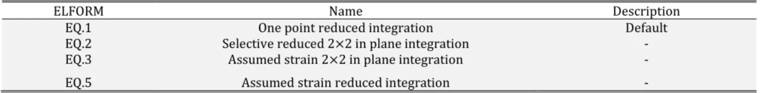
Table 2: Formulations of thick-shell elements in LS-DYNA.
ELFORM Name Description
EQ.1 One point reduced integration Default
EQ.2 Selective reduced 2×2 in plane integration -
EQ.3 Assumed strain 2×2 in plane integration -
The thickness enhanced shell formulation is also based on Reissner-Mindlin kinematic assumption with one-point integration and bi-linear nodal interpolation (EQ. 25). In the case of EQ. 26, a 2×2 integration in the shell element plane is adopted while the Bathe-Dvorkin transverse shear correction helps to eliminate W-mode hour-glassing. In addition, the linear strain through thickness feature is adopted.
The details of abovementioned four representative thin-shell element models are as described by Haufe et al. (2013).
The thick-shell elements shown in Table 2 can also be categorised as follows. This thick-shell element based on 8-node shell/solid is considered to be between thin-shell and solid element. The thin-thick shells (EQ. 1 and 2) are composed of 8-node shells with 2D stress state similar to that of thin shell. Basically, a penalty function is adopted to constrain the element thickness between top and bottom nodes. Once membrane stress is applied, only then can element thickness be changed. In general, the thin-thick shells depicted in Table 2 (EQ. 1 and 2) are not recommended due to efficiency issues in comparison to thin shells in Table 1.
Thick-thick shells (EQ. 3 and 5) also adopts the 8-node shell/solid, but is presumed to be under 3D stress state. In this case, the element thickness matter is resolved, which can be changed by thickness stress, however, it requires an extremely long computational time. In the case of EQ. 5, shear locking and hourglass issues are resolved and the laminated shell theory is applicable. This essentially helps to solve the engineering problem of bending with one element over thickness. It is developed for modelling thick composite structures whereby improper element ratio can also be considered.
2.2 Solid elements
Table 3 shows the solid element formulations. There are several types of elements, however, only few are ac-centuated in the present study.
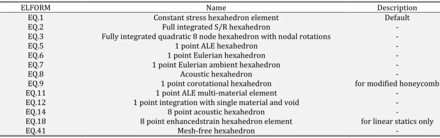
Table 3: Formulations of solid elements in LS-DYNA.
ELFORM Name Description
EQ.1 Constant stress hexahedron element Default
EQ.2 Full integrated S/R hexahedron -
EQ.3 Fully integrated quadratic 8 node hexahedron with nodal rotations -
EQ.5 1 point ALE hexahedron -
EQ.6 1 point Eulerian hexahedron -
EQ.7 1 point Eulerian ambient hexahedron -
EQ.8 Acoustic hexahedron -
EQ.9 1 point corotational hexahedron for modified honeycomb
EQ.11 1 point ALE multi-material element -
EQ.12 1 point integration with single material and void -
EQ.14 8 point acoustic hexahedron -
EQ.18 8 point enhancedstrain hexahedron element for linear statics only
EQ.41 Mesh-free hexahedron -
A standard element (=EQ. 1) is set as the default, which consists of 8-node hexahedron solid element with tri-linear shape functions. It adopts reduced integration, i.e., one-point integration in the middle of the element. A fully integrated element (=EQ. 2) is similar to the default element. This element adopts eight integration points which consumes 2-3 times additional computational cost than that of EQ. 1. It considers hourglass mode issues but may bring about shear locking and lower deformation problems.
3. TARGET STRUCTURE
3.1 Blast wall design
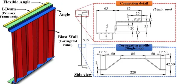
Figure 1: Configuration of the target blast wall model.
Blast wall structures are integrated installations on offshore topsides to minimise the effects of explosive load-ing. The present blast wall model was appropriated from a research report by HSE (2003), who provided relevant experiment data that are beneficial to this study. In addition, various studies on blast wall analysis and design op-timisation have recently been conducted by several researchers (Kim et al., 2014; Hedayati et al., 2015; Syed et al., 2016; Li et al., 2017; Hao et al., 2017). The configuration and dimensions of the target blast wall consisting of a corrugated panel and connecting parts including angle, flexible angle, and I-beams are shown in Figure 1. In addi-tion, this blast wall is a ¼ scale model of the real structure that was constructed and tested by HSE (2003).
The material properties, i.e., material type, density, elastic modulus, yield strength, and Cowper-Symonds co-efficients, are summarized in Figure 2. The Cowper-Symonds constitutive equation in Eq. (1) proposed by Cowper and Symonds (1957) is commonly applied in the ships and offshore industry (Park et al., 2015a; 2015b; Choi et al., 2016; Kim et al., 2018) to consider the dynamic or strain rate effects, which are obtained via dynamic tensile tests.
11 q
Y d Y C
Eq. (1)
where Yd= dynamic yield strength,Y = static yield strength,
= strain rate,C
andq
= Cowper-Symondscoefficients obtained through curve-fitting. The dynamic characteristics of the materials are illustrated by the plot of dynamic yield strength normalised by static yield strength versus strain rate in Figure 2.
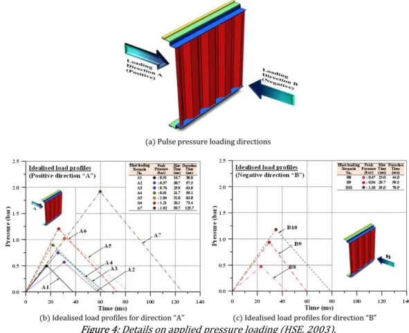
3.2 Applied blast loading
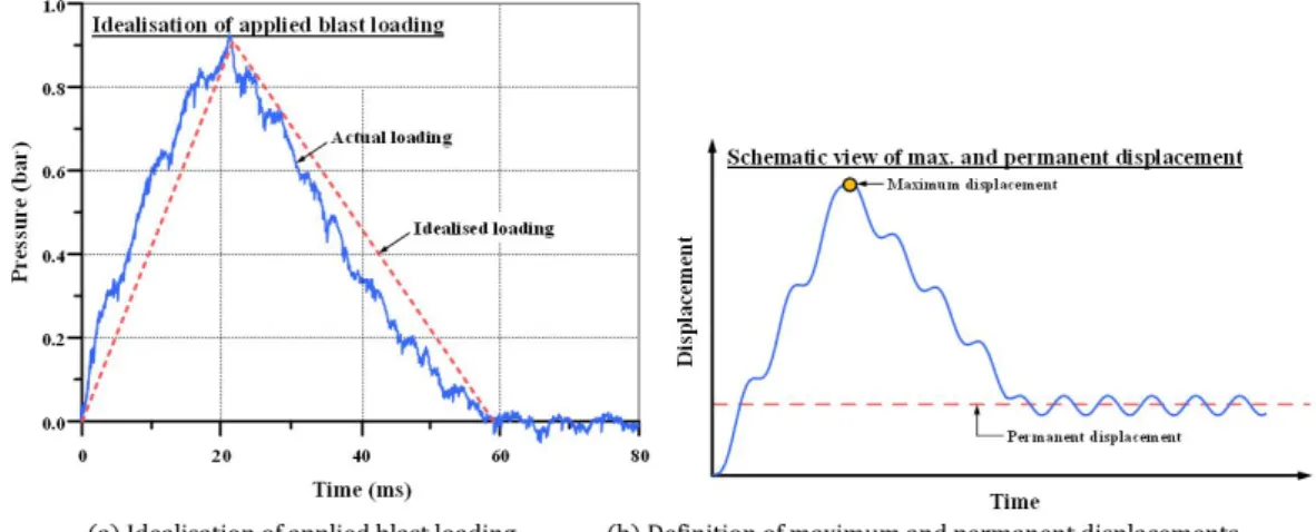
The applied blast loadings were idealised as triangular load curves by noting the rise time, tr duration time, td
and peak pressure, ppeak as shown in Figure 3(a) as inputs into the numerical pre-processor. The maximum and
permanent mid-span displacements are also demonstrated in Figure 3(b).
Figure 3: Processing of FEA input and output data.
4. APPLIED EXAMPLE
In the present section, performance of pre-selected LS-DYNA element types, i.e. thin-shell, thick-shell and solid for modelling of the target blast wall were investigated through which relevant finite element (FE) formulations were selected for further numerical studies with recommendations.
4.1 Experimental test results
Figure 4: Details on applied pressure loading (HSE, 2003).
Table 4: Summary of pulse pressure tests by HSE (2003).
peak
p (bar)
Loading direction tr
(ms)
d t
(ms)
max
w
(mm)
p
w (mm)
0.51 (A1) A
(Positive) 16.7 38.0 4.8 0.0
0.57 (A2) 30.7 57.5 4.9 0.0
0.76 (A3) 25.9 63.0 7.5 0.0
0.91 (A4) 21.7 59.1 7.5 0.0
1.04 (A5) 31.0 83.0 9.0 0.0
1.21 (A6) 26.1 73.4 - 4.0
1.92 (A7) 59.7 125.7 - 69.0
0.47 (B8) B
(Negative) 23.0 44.0 2.5 0.0
0.94 (B9) 29.7 59.5 8.3 1.0
1.18 (B10) 30.8/41.2 78.9 - 283.0
Note: ppeak= peak pressure, tr= rise time, td= duration time, wmax= maximum deflection, and wp= permanent deflection.
4.2 Numerical modelling
In ensuring robustness and safety of offshore structures, the possibilities of failure due to accidents such as explosion or fire should be anticipated and clearly reflected in the design stage. Due to high costs and time restraints, numerical methods such as nonlinear finite element method (NLFEM) are widely favoured in the offshore industry to ascertain structural responses, in contrast to experimental or destructive testing.
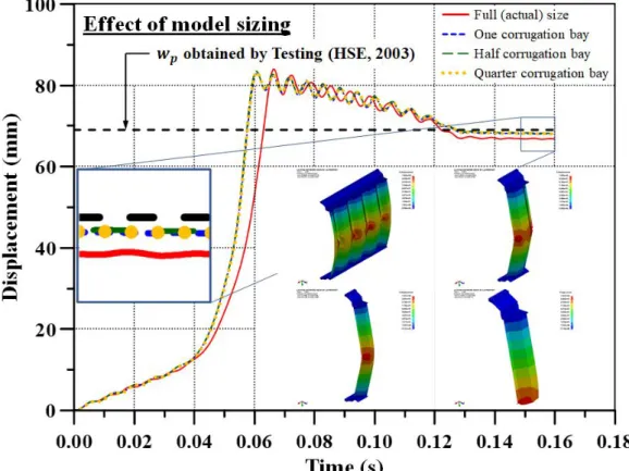
Figure 5: Benchmark study of FE model size based on extreme load condition, i.e. loading scenario A7.
LS-DYNA explicit FE solver was used to perform the numerical simulation. The structural responses of the blast wall model subjected to a range of pulse pressure load profiles illustrated in Fig. 4 were evaluated. Pertaining to boundary conditions, the upper edge of the model was assumed to be fixed with both sides of the model set to be symmetrical in the transverse direction; the bottom edges were set to be symmetrical in the longitudinal direction, while a uniformly-distributed time-dependent idealised pulse pressure loading was applied all over the surface of the corrugated panel, as illustrated in Figure 6.
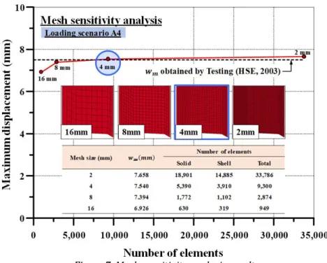
In the previous study by Sohn et al. (2012), 4mm of mesh size was adopted to the entire FE model. For the confirmation, mesh sensitivity analysis was conducted by adopting 2 mm, 4 mm, 8 mm, and 16 mm of mesh sizes in the present study shown in Figure 7. From the obtained results, we have confirmed that 4 mm of mesh size is relevant to be applied to FE modelling of the blast wall.
Figure 7: Mesh sensitivity analysis result.
Material model No. 24 in LS-DYNA was used to represent the nonlinear dynamic behaviour of the structure by specifying the material strain rate parameters.
4.3 Assessment of FE types and FE formulations in LS-DYNA
This section is divided into two parts. First, the assessment and selection of FE types, i.e. solid, thin-shell, and thick-shell are addressed in section 4.3.1, from which further assessment of the selected FE types are discussed in the context of performance of FE formulations, i.e. reduced or full integration, and hourglass control in section 4.3.2. The structural responses, i.e. maximum and permanent displacements were validated against the test results (HSE, 2003). In addition, the obtained outcomes were discussed based on accuracy of numerical simulation results as well as computational cost.
4.3.1 Selection of FE types
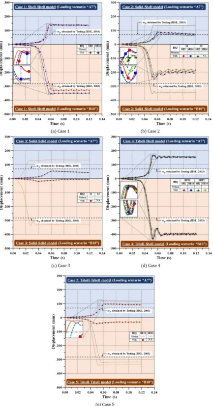
Five (5) representative cases as shown in Table 5 were generated to study the blast response of target blast wall models based on combinations of pre-selected quadrilateral thin- and thick-shell, and hexahedral solid finite elements in LS-DYNA. Fig. 8 provides an overview of blast responses for extreme load scenarios in both loading directions, i.e. A7 (ppeak=1.92 bar) and B10 (ppeak=1.18 bar) for each of the five cases in terms of peak structural
displacements, with respect to experimental measurements provided in Table 4.
Table 5: Assumed finite element types for modelling of the blast wall structure.
FE
Formulation Case 1 Case 2 Case 3 Case 4 Case 5
Supporting members Shell (SH) Solid (S) Solid (S) T-Shell (SHT) T-Shell (SHT)
Corrugated panel Shell (SH) Shell (SH) Solid (S) Shell (SH) T-Shell (SHT)
Figure 8: Displacement-time plots for Cases 1-5 models (Table 5 can be referred to for the naming of each model).
Figure 9: Statistical analysis results between testing and obtained outcomes (Table 5 can be referred).
In Fig. 9(b), mean and COV values could not calculated because zero (0) deformation was measured from the testing. Therefore, FEA/test could not be done. In this regard, R2 and S values were added on behalf of mean and COV values for the comparison. With regards to the accuracy of numerical simulation, models from Case 1 or Case 2 model may be suggested for further analyses based on the obtained outcomes as presented in Figs. 9(a) and (b). Furthermore, the performance of all cases can be sorted in the sequence of increasing computational costs as Case 1 (Cheap)< Case 2 < Case 3 < Case 4 < Case 5 (Expensive), while the details are referred to Table B.1 in the Ap-pendix part. Throughout this study, the Intel® Core™ i7-6800K CPU @ 3.40GHz computer processor with 64-bit Operating system was used.
Therefore, in this section which covers “Selection of FE types”, Case 1 and Case 2 can be recommended to users like structural designers for the analysis of offshore blast wall structure subjected to explosive loading. More details on Case 2 which apparently gives higher accuracy than Case 1 is scrutinised in the next section.
4.3.2 Selection of FE formulations
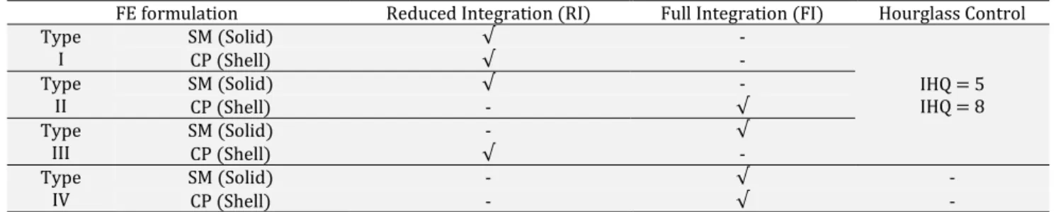
In section 4.3.1, shell and solid elements were recommended for modelling corrugated panel and connection parts, accordingly. In this section, the performance of several pre-selected FE formulations will be assessed. Table 6 shows four (4) FE models, comprising the combinations of reduced- and full- integration of solid and shell ele-ments - systematically Types I, II, III, and IV - for detailed investigation. Each FE model is named according to the designation of FE formulations in LS-DYNA (refer to section 2) in the following sequence: supporting members-corrugation panel-hourglass control.
For example, S1-SH16-8 refers to a model consisting of reduced integration solid supporting members and full integration shell corrugated panel with hourglass control EQ.8, while S3-SH2-0 refers to one consisting full integra-tion solid supporting members and reduced integraintegra-tion shell corrugated panel without hourglass control. Table 5 is referred for the abbreviations.
Table 6: Selected combinations for the assessment of performance of shell and solid FE formulations.
FE formulation Reduced Integration (RI) Full Integration (FI) Hourglass Control
Type
I SM (Solid) √ -
IHQ = 5 IHQ = 8
CP (Shell) √ -
Type
II SM (Solid) CP (Shell) √ - √ -
Type
III SM (Solid) CP (Shell) √ - √ -
Type
IV SM (Solid) CP (Shell) - - √ √ - -
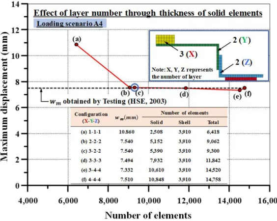
For the relatively thicker connection parts (supporting members), the number of through thickness solid ele-ments can be another factor that influences the numerical results. Figure 10 demonstrates the relationship between several configurations of through thickness element distribution and the maximum midspan displacement (HSE, 2003), which clearly indicates that at least two layers of elements are required for a proper representation of the bending behaviour. Thus, for efficient FE simulations, configuration (c) with 3, 2, and 2 layers of elements through the thicknesses of I-beam, flexible angle, and angle, respectively, has been adopted for all the following FE models in this study.
Figure 10: Effect of number of through thickness solid elements on the numerical accuracy.
Through comparisons with the test results (HSE, 2003), it was observed that the influence of FE formulations rises exponentially with increasing peak pressure. Figure 11(a) compares the displacement-time histories of all models (Types I to IV) subjected to 1.92 bar peak pressure (loading scenarioA7), which clearly indicates the capa-bilities of these FE formulations in predicting the dynamic responses of the blast wall model.
The excessively overestimated responses from Type I (S1-SH2-0) and Type II (S1-SH16-0) models were due to the hourglass modes that generated zero energy in the affected solid elements, particularly at regions of large deformation, causing the connection angles to lose stiffness hence exaggerating the maximum response. The hour-glassing phenomenon is shown in Figure 11(b). While reduced integration (RI) hexahedral solid and quadrilateral shell elements are prone to hourglassing, Type III model (S3-SH2-0) was effective in mitigating the undesirable elemental “defects” in most cases that were subjected to low peak pressures.
For instance, the permanent displacements in loading scenario A7 was slightly underestimated by the fully-integrated (FI) solid elements, which might be due to the shear-locking phenomenon that over-stiffens the re-sponses. In addition, the effect of number of integration point, which caused the different outcomes, should also be carefully taken into consideration; the hourglass mode can occur if only one (1) integration point is adopted for the FE simulation. Furthermore, relevant additional options may be required to prevent hourglass mode.
S1-SH2-0 and S1-SH16-0, a simple deduction can be made such that RI solids would suffer the numerical shortcom-ings, in which they tend to be excessively flexible, hence the overestimation of permanent displacement. However, hourglassing did not occur in the FI solids shown in Figure 11(b) - connection part modelled by solid element.
Figure 11: FEA outcomes of Type I-IV models without hourglass control (loading scenario A7).
in LS-DYNA were applied in accordance to Table 6, to all models. Basically, under-integrated solid and shell ele-ments are prone to hourglass modes, which can be handled in two ways, e.g. by applying hourglass control functions in LS-DYNA and/or by mesh refinement.
Figures 12(a) and (b) present the extent of hourglassing in terms of hourglass energies generated in the solid and shell elements, respectively, with respect to element mesh size of a representative analysis case. It is evident that the hourglass energy is directly related the fineness of element mesh, though this aspect of modelling is often insignificant for shell elements due to the location of integration points. As a rule of thumb, the generated hourglass energy in an element shall be well below one-tenth (or 10%) of the total energy generated in that element. Findings in Figure 12 agreed well with the adopted mesh size as shown in Figure 7.
Figure 12: Relationship between hourglass energies of shell and solid elements and element mesh size.
Figure 13: FEA results of Type I-III models with hourglass control (loading scenario A7).
Due to advantages in computational efficiency and ability to overcome shear locking, RI schemes are widely implemented in explicit FEA codes. However, the downside of these elements is their tendency to introduce hour-glass modes of deformation, in which neither stresses nor strains are generated in the affected elements, thus ill-defining the resulting structural response.
While FI elements are effective in dealing with hourglass instabilities, their major drawback is, as opposed to that of RI elements, over-stiffening of the responses by shear-locking. In short, shear locking and hourglassing are two compromised factors between the two integration schemes. Thus, as it may be difficult to eliminate hourglass-ing, some form of hourglass control is required in the FEA.
Figure 14: Statistical analysis results between FEA outcome and test data (HSE, 2003).
As S1-SH2-0 and S1-SH16-0 were affected by hourglassing, their calculations are unaccredited and the values shown in Figures 14(a) and (b) were discarded. From Figure 14(a), Types I and II with slightly higher R2-values performed well in predicting maximum displacements compared to slightly underperformed Types III and IV, while from Figure 14(b), Types III and IV have somewhat outperformed Types I and II in predicting permanent displace-ments. However, though with decent capabilities, Types III and IV models were deemed too conservative in dealing with cases involving high peak pressures, in addition to requiring much higher computational costs as shown in Table B.2 (Appendix B).
Type IV (Expensive) < Type III < Type II < Type I (Cheap)
Comparing the computational cost, the same PC has been used as mentioned in Section 4.3.1 and the following order is defined. Thus, the use of RI elements with appropriate hourglass control function is indeed recommended for cost-effective solutions.
5. CONCLUDING REMARKS
In the present study, the influences of solid and shell FE formulations with additional hourglass control func-tions on the maximum responses of corrugated blast wall has been investigated using LS-DYNA explicit finite ele-ment solver. It is wise to take advantage of thickness variation over the entire target structure when selecting the representative finite element (FE) types, i.e. thin-shell, thick-shell or solid to represent the model parts.
The selection of element integration scheme, similar to other considerations in FE modelling, is essential to the quality of FEA solutions. Reduced integration (RI) elements are favourable in explicit dynamics analyses, given its high speed and robustness under high structural distortions, whereas full integration (FI) elements are more typi-cal in implicit analyses. Although FI solid elements perform consistently well in predicting maximum responses under low peak pressure, they are very costly compared to their RI counterparts.
Furthermore, FI solid elements are not suitable for predicting responses of high peak pressure as the effect of shear locking increasingly falsifies or over-stiffens the responses, which had been observed through the compari-son with experimental measurements. Moreover, the number of integration points should also be carefully taken into consideration in order to prevent the shear locking phenomenon of solid element.
In contrast, RI solid elements associated with relevant hourglass control functions can be used to obtain satis-factory estimations of blast responses for all peak pressures in much shorter computation times. The present rec-ommendations are presumably software independent and generally govern different FE software.
ACKNOWLEDGEMENTS
This study was supported by the Technology Innovation Program (Grant No.: 10051279) funded by the Min-istry of Trade, Industry & Energy (MI, Korea) and Universiti Teknologi PETRONAS (0153AA-E60 and 0153AB-M55). The authors would like to thank for the great support of POSTECH, and UTP. Some part of the present study was presented in the 1st International Conference on Architecture and Civil Engineering (ICACE 2017), 8-9 May, Kuala Lumpur, Malaysia and all the presented papers have been published in ARPN Journal of Engineering and Applied Science (Ng and Hwang, 2017).
REFERENCES
Biggs, J.M. (1964). Introduction to structural dynamics, McGraw-Hill Companies (New York).
Boh, J., Choo, Y., Louca, L. (2004). Design and numerical assessment of blast walls subjected to hydrocarbon explo-sions. The 14thInternational Offshore and Polar Engineering Conference (ISOPE 2004), 23-28 May, Toulon, France.
Choi, H.S., Shin, G., Choung, J.M., Kim, K.H., Seo, D.W., Kim, K.S., Wong, E.W.C., Kim, D.K. (2016). Numerical simulation of high Manganese steel FLNG storage tank damaged by collision. The 3rd International Conference on Ocean, Me-chanical and Aerospace for Scientist and Engineer (OMAse 2016), 7-8 November, Kuala Terengganu, Malaysia.
Cowper, G.R., Symonds, P.S. (1957). Strain-hardening and strain-rate effects in the impact loading of cantilever beams. Technical Report No. 28, Division of Applied Mathematics, Brown University (Providence, Rhode Island).
FABIG. (1999). Design guide for stainless steel blast walls, Technical note 5 (Edited by @ Brewerton, R.), Fire and Blast Information Group, Berkshire, UK.
Hao, Y., Hao, H., Shi, Y., Wang, Z., Zong, R. (2017). Field Testing of Fence Type Blast Wall for Blast Load Mitigation.
International Journal of Structural Stability and Dynamics In-press.
https://doi.org/10.1142/S0219455417500997
Haufe, A., Schweizerhof, K., DuBois, P. (2013). Properties & limits: review of shell element formulations. LS-DYNA Developer Forum 2013, 24 September, Filderstadt, Germany.
Hedayati, M.H., Sriramula, S., Neilson, R.D. (2015). Reliability of Profiled Blast Wall Structures. In: Kadry S., El Hami A. (Eds) Numerical Methods for Reliability and Safety Assessment, Springer International Publishing, Switzerland. https://doi.org/10.1007/978-3-319-07167-1_13
HSE. (2000). Modelling failure of welded connections to corrugated panel structures under blast loading (Edited by L.A.Louca and J.Friis), Imperial College of Science, Technology and Medicine, Health and Safety Executive, UK.
HSE. (2003). Pulse pressure testing of 1/4 scale blast wall panels with connections. Research Report 124 (Edited by Schleyer, G.K. and Langdon, G.S.), Liverpool University, Health and Safety Executive, Liverpool, UK.
Kim, D.K., Ng, W.C.K., Hwang, O.J. (2018). An empirical formulation to predict maximum deformation of blast wall under explosion. Structural Engineering and Mechanics, accepted for publication.
Kim, J.H. (2014). A new procedure for fire structural assessment of offshore installations, PhD Dissertation, Pusan National University, Busan, Republic of Korea.
Kim, S.J., Sohn, J.M., Lee, J.C., Li, C.B., Seong, D.J., Paik, J.K. (2014). Dynamic Structural Response Characteristics of Stiffened Blast Wall under Explosion Loads. Journal of the Society of Naval Architects of Korea 51(5): 380-387.
Koh, B.C., Kikuchi, N. (1987). New improved hourglass control for bilinear and trilinear elements in anisotropic linear elasticity. Comp. Methods in Applied Mechanics and Eng. 65: 1-46
Langdon, G.S., Schleyer, G.K. (2005a). Inelastic deformation and failure of profiled stainless steel blast wall panels. Part I: experimental investigations. Int. J. Impact Eng. 31: 341-369.
Langdon, G.S., Schleyer, G.K. (2005b). Inelastic deformation and failure of profiled stainless steel blast wall panels. Part II: analytical modelling considerations. Int. J. Impact Eng. 31: 371-399.
Langdon, G.S., Schleyer, G.K. (2006). Deformation and failure of profiled stainless steel blast wall panels. Part III: finite element simulations and overall summary. Int. J. Impact Eng. 32: 988-1012.
Langer, P., Maeder, M., Guist, C., Krause, M., Marburg, S. (2017). More than six elements per wavelength: the practical use of structural finite element models and their accuracy in comparison with experimental results. J. Comp. Acous-tics 25: 1750025-1-23.
Li, J., Ma, G., Hao, H., Huang, Y. (2017). Optimal blast wall layout design to mitigate gas dispersion and explosion on a cylindrical FLNG platform. Journal of Loss Prevention in the Process Industries 49(Part B): 481-492.
Louca, L.A., Boh, J.W., Choo, Y.S. (2004). Design and analysis of stainless steel profiled blast barriers. J. Construc-tional Steel Res. 60: 1699-1723.
LS-DYNA, (2014). LS-DYNA Theoretical Manual, Livermore Software Technology Corporation (Livermore, CA).
Macneal, R.H., Harder, R.L. (1985). A proposed standard set of problems to test finite element accuracy. Finite Ele-ments in Analysis and Design 1: 3-20.
Ng, W.C.K., Hwang, O.J. (2017). Effect of finite element formulation type on blast wall analysis subjected to explosive loading. ARPN Journal of Engineering and Applied Sciences 12: 5778-5783.
Park, D.K., Kim, D.K., Park, C.H., Park, D.H., Jang, B.S., Kim, B.J., Paik, J.K. (2015a). On the crashworthiness of steel-plated structures in an Arctic environment: An experimental and numerical study. Journal of Offshore Mechanics and Arctic Engineering 137: 051501-1-15.
Park, D.K., Kim, D.K., Seo, J.K., Kim, B.J., Ha, Y.C., Paik, J.K. (2015b). Operability of non-ice class aged ships in the Arctic Ocean – Part II: Accidental limit state approach. Ocean Engineering 102: 206-215.
Schwer, L.E., Key, S.W., Pucik, T.A., Bindeman, L.P. (2005). An assessment of the LS-DYNA hourglass formulations via the 3D patch test. 5th European LS-DYNA Users Conference, 25-26 May, Birmingham, UK.
Sohn, J.M., Kim, B.H., Paik, J.K., Schleyer, G.K. (2012). Nonlinear structural consequence analysis of blast wall struc-tures under hydrocarbon explosive loads. The 31stInternational Conference on Ocean, Offshore and Arctic Engi-neering (OMAE 2012), 1-6 July, Rio de Janeiro, Brazil.
Sohn, J.M., Kim, S.J., Kim, B.H., Paik, J.K. (2013). Nonlinear structural consequence analysis of FPSO topside blast-walls. Ocean Eng. 60: 149-162.
Sun, E.Q. (2006). Shear locking and hourglassing in MSC Nastran, ABAQUS, and ANSYS. Proceedings of MSC Soft-ware Corporation's 2006 Americas Virtual Product Development Conference, Detroit, MI, USA.
APPENDIX A. SELECTION OF FE TYPES (CASE 1-5)
(Note: COV = Coefficient of variation, R2 = Coefficient of determination, S = Standard error of regression)
Nopressure (bar)Peak
Case 1 - Shell-Shell model (Maximum displacement)
Test (mm)
FEA (mm) FEA/Test
S2 -S2 -0
S2 -S2 -5
S16 -S16
-0
S16 -S16 -8
S2 -S2 -0
S2 -S2 -5
S16 -S16
-0
S16 -S16
-8
1 0.51 4.8 5.007 5.007 5.005 5.005 1.043 1.043 1.043 1.043
2 0.57 4.9 5.298 5.299 5.296 5.297 1.081 1.081 1.081 1.081
3 0.76 7.5 7.554 7.554 7.548 7.549 1.007 1.007 1.006 1.006
4 0.91 7.5 8.450 8.391 8.395 8.396 1.127 1.119 1.119 1.119
5 1.04 9.0 10.658 10.090 10.240 10.233 1.184 1.121 1.138 1.137
6 1.21 - 16.348 14.028 14.758 14.762 - - -
-7 1.92 - 142.570 142.340 140.680 140.920 - - -
-8 -0.47 -2.5 -4.608 -4.608 -4.603 -4.604 1.843 1.843 1.841 1.841
9 -0.94 -8.3 -10.753 -10.296 -10.430 -10.434 1.296 1.240 1.257 1.257
10 -1.18 - -357.440-334.340-352.420-351.670 - - -
-Mean 1.226 1.208 1.212 1.212
COV 0.235 0.240 0.238 0.238
R2 0.99620.99610.99630.9963
S 0.52820.51760.50890.5077
Mean (Average) 1.215
COV (Average) 0.238
R2 (Average) 0.9962
S (Average) 0.5156
No Peak pressure (bar)
Case 1 - Shell-Shell model (Permanent displacement)
Test (mm)
FEA (mm) FEA/Test
S2 -S2 -0
S2 -S2 -5
S16 -S16 -0
S16 -S16
-8
S2 -S2 -0
S2 -S2 -5
S16 -S16
-0
S16 -S16
-8
1 0.51 0.0 0 0 0 0 N/A N/A N/A N/A
2 0.57 0.0 0 0 0 0 N/A N/A N/A N/A
3 0.76 0.0 0 0 0 0 N/A N/A N/A N/A
4 0.91 0.0 0.210 0 0 0 N/A N/A N/A N/A
5 1.04 0.0 1.240 0.549 0.739 0.727 N/A N/A N/A N/A
6 1.21 4.0 5.980 2.960 4.000 4.000 1.495 0.740 1.000 1.000
7 1.92 69.0 138.0 137.0 136.0 136.0 2.000 1.986 1.971 1.971
8 -0.47 0.0 0 0 0 0 N/A N/A N/A N/A
9 -0.94 -1.0 -0.957 -0.447 -0.549 -0.550 0.957 0.447 0.549 0.550
10 -1.18 -283.0 -355.000 -330.000 -351.000 -350.000 1.254 1.166 1.240 1.237
Mean N/A N/A N/A N/A
COV N/A N/A N/A N/A
R2 0.9852 0.9793 0.9852 0.9850
S 16.1311 17.9067 15.9215 15.9984
Mean (Average) N/A
COV (Average) N/A
R2 (Average) 0.9837
S (Average) 16.4894
No Peak pressure (bar)
Case 2 - Solid-Shell model (Maximum displacement)
Test (mm)
FEA (mm) FEA/Test
S1 -SH2 -0 S1 -SH2 -5 S1 -SH16 -0 S1 -SH16 -8 S3 -SH2 -0 S3 -SH2 -5 S3 -SH16 -0 S1 -SH2 -0 S1 -SH2 -5 S1 -SH16 -0 S1 -SH16 -8 S3 -SH2 -0 S3 -SH2 -5 S3 -SH16 -0
1 0.51 4.8 5.105 4.947 5.103 4.945 4.844 4.844 4.842 1.064 1.031 1.063 1.030 1.009 1.009 1.009
2 0.57 4.9 5.433 5.248 5.429 5.246 5.162 5.162 5.159 1.109 1.071 1.108 1.071 1.053 1.053 1.053
3 0.76 7.5 7.794 7.343 7.787 7.337 7.057 7.057 7.049 1.039 0.979 1.038 0.978 0.941 0.941 0.940
4 0.91 7.5 9.396 8.042 9.334 8.034 7.788 7.821 7.818 1.253 1.072 1.245 1.071 1.038 1.043 1.042
5 1.04 9.0 12.052 9.948 11.800 9.983 9.846 9.735 9.767 1.339 1.105 1.311 1.109 1.094 1.082 1.085
6 1.21 - 20.149 13.181 18.831 13.401 13.192 12.623 12.824 - - -
-7 1.92 - 140.230 86.773138.960 84.59675.434 74.088 72.951 - - -
-8 -0.47 -2.5 -4.771 -4.474 -4.765 -4.471 -4.370 -4.370 -4.367 1.908 1.790 1.906 1.788 1.748 1.748 1.747
9 -0.94 -8.3 -12.425 -9.833 -12.156 -9.888 -9.543 -9.421 -9.463 1.497 1.185 1.465 1.191 1.150 1.135 1.140
10 -1.18 - -357.90-246.00-357.20-252.66-241.82-227.37-232.64 - - -
-Mean 1.315 1.176 1.305 1.177 1.148 1.144 1.145
COV 0.235 0.236 0.234 0.236 0.238 0.238 0.238
R2 0.99410.99530.99470.99540.99420.99400.9941
S 0.73430.55200.68040.54620.59410.60080.5980
Mean (Average) 1.202
COV (Average) 0.236
R2 (Average) 0.9945
S (Average) 0.6151
No
Peak
pres-sure (bar)
Case 2 - Solid-Shell model (Permanent displacement)
Test (mm)
FEA (mm) FEA/Test
S1 -SH2 -0 S1 -SH2 -5 S1 -SH16 -0 S1 -SH16 -8 S3 -SH2 -0 S3 -SH2 -5 S3 -SH16 -0 S1 -SH2 -0 S1 -SH2 -5 S1 -SH16 -0 S1 -SH16 -8 S3 -SH2 -0 S3 -SH2 -5 S3 -SH16 -0
1 0.51 0.0 0 0 0 0 0 0 0 N/A N/A N/A N/A N/A N/A N/A
2 0.57 0.0 0 0 0 0 0 0 0 N/A N/A N/A N/A N/A N/A N/A
3 0.76 0.0 0.153 0 0.167 0 0 0 0 N/A N/A N/A N/A N/A N/A N/A
4 0.91 0.0 0.848 0 0.714 0 0.107 0.032 0 N/A N/A N/A N/A N/A N/A N/A
5 1.04 0.0 2.550 0.564 2.240 0.636 0.825 0.520 0.658 N/A N/A N/A N/A N/A N/A N/A
6 1.21 4.0 10.000 2.400 8.470 2.720 3.020 2.210 2.520 2.500 0.600 2.118 0.680 0.755 0.553 0.630
7 1.92 69.0 135.00068.700135.000 68.10058.600 57.800 57.800 1.957 0.996 1.957 0.987 0.849 0.838 0.838
8 -0.47 0.0 0 0 0 0 0 0 0 N/A N/A N/A N/A N/A N/A N/A
9 -0.94 -1.0 -2.260 -0.346 -2.000 -0.404 -0.471 -0.322 -0.405 2.260 0.346 2.000 0.404 0.471 0.322 0.405
10 -1.18 -283.0 -347.00-196.00 -346.00-205.00-192.00-183.00-189.00 1.226 0.693 1.223 0.724 0.678 0.647 0.668
Mean N/A N/A N/A N/A N/A N/A N/A
COV N/A N/A N/A N/A N/A N/A N/A
R2 0.98540.99160.98520.99420.99720.99610.9971
S 15.65316.588515.76545.69343.66384.14963.6740
Mean (Average) N/A
COV (Average) N/A
R2 (Average) 0.9924
S (Average) 7.8840
No pressure Peak (bar)
Case 3 - Solid-Solid model (Maximum displacement)
Test (mm)
FEA (mm) FEA/Test
S1 -S1 -0
S1 -S1 -5
S3 -S3 -0
S1 -S1 -0
S1 -S1 -5
S3 -S3 -0
1 0.51 4.8 96.184 4.953 4.825 20.038 1.032 1.005
2 0.57 4.9 114.090 5.259 5.144 23.284 1.073 1.050
3 0.76 7.5 130.030 7.278 7.013 17.337 0.970 0.935
4 0.91 7.5 136.980 7.922 7.805 18.264 1.056 1.041
5 1.04 9.0 131.600 9.832 9.778 14.622 1.092 1.086
6 1.21 - 139.430 12.803 12.932 - -
-7 1.92 - 133.340 53.455 52.146 - -
-8 -0.47 -2.5 -317.050 -4.554 -4.345 126.820 1.821 1.738
9 -0.94 -8.3 -339.410 -10.157 -9.452 40.893 1.224 1.139
10 -1.18 - -340.060 -21.740 -19.446 - -
-Mean 37.323 1.181 1.142
COV 1.083 0.248 0.237
R2 0.9084 0.9958 0.9940
S 72.9819 0.5231 0.5997
Mean (Average) 13.215
COV (Average) 0.522
R2 (Average) 0.9661
S (Average) 24.7016
No pressure Peak (bar)
Case 3 - Solid-Solid model (Permanent displacement)
Test (mm)
FEA (mm) FEA/Test
S1 -S1 -0
S1 -S1 -5
S3 -S3 -0
S1 -S1 -0
S1 -S1 -5
S3 -S3 -0
1 0.51 0.0 89.400 0 0 N/A N/A N/A
2 0.57 0.0 109.000 0 0 N/A N/A N/A
3 0.76 0.0 126.000 0 0 N/A N/A N/A
4 0.91 0.0 134.000 0 0.102 N/A N/A N/A
5 1.04 0.0 129.000 0.460 0.690 N/A N/A N/A
6 1.21 4.0 136.000 2.130 2.770 34.000 0.533 0.693
7 1.92 69.0 132.000 40.700 40.100 1.913 0.590 0.581
8 -0.47 0.0 -313.000 0 0 N/A N/A N/A
9 -0.94 -1.0 -326.000 -0.352 -0.473 326.000 0.352 0.473
10 -1.18 -283.0 -328.000 -7.220 -7.670 1.159 0.026 0.027
Mean N/A N/A N/A
COV N/A N/A N/A
R2 0.3010 0.2471 0.2607
S 190.847 12.217 11.965
Mean (Average) N/A
COV (Average) N/A
R2 (Average) 0.2696
S (Average) 71.6761
No Peak pres-sure (bar )
Case 4 - Tshell-Shell model (Maximum displacement)
Test (mm )
FEA (mm) FEA/Test
SHT1 -SH2 -0 SHT1 -SH2 -5 SHT1 -SH16 -0 SHT1 -SH16 -8 SHT2 -SH2 -0 SHT2 -SH2 -5 SHT2 -SH16 -0 SHT2 -SH16 -8 SHT1 -SH2 -0 SHT1 -SH2 -5 SHT1 -SH16 -0 SHT1 -SH16 -8 SHT2 -SH2 -0 SHT2 -SH2 -5 SHT2 -SH16 -0 SHT2 -SH16 -8
1 0.51 4.8 5.365 5.355 5.361 5.352 5.357 5.357 5.354 5.354 1.1181.1161.1171.1151.1161.1161.1151.115
2 0.57 4.9 6.255 6.233 6.246 6.225 6.239 6.239 6.231 6.231 1.2771.2721.2751.2701.2731.2731.2721.272
3 0.76 7.5 8.440 8.387 8.430 8.384 8.404 8.393 8.391 8.388 1.1251.1181.1241.1181.1211.1191.1191.118
4 0.91 7.5 11.369 10.853 11.213 10.912 11.129 10.915 10.943 10.986 1.5161.4471.4951.4551.4841.4551.4591.465
5 1.04 9.0 14.904 13.087 14.270 13.337 14.287 13.254 13.558 13.561 1.6561.4541.5861.4821.5871.4731.5061.507
6 1.21 - 31.603 20.191 28.180 21.061 28.542 21.121 23.698 23.720 - - -
-7 1.92 - 168.850 165.860 167.560 164.340 168.410 168.260 166.990 166.910 - - -
-8 0.47- -2.5 -5.537 -5.518 -5.529 -5.511 -5.524 -5.524 -5.516 -5.516 2.2152.2072.2122.2042.2102.2102.2062.206
9 0.94- -8.3 -14.057-13.093-13.731-13.283-13.809-13.175-13.368-13.3841.6941.5771.6541.6001.6641.5871.6111.613
101.18- - 437.73
-0 -436.05 0 -437.26 0 -436.20 0 -437.67 0 -436.60 0 -436.94 0 -436.81
0 - - -
-Mean 1.5141.4561.4951.4641.4941.4621.4701.471
COV 0.2570.2570.2560.2570.2570.2570.2560.256
R2 0.983
6 0.9907 0.9865 0.9901 0.9867 0.9902 0.9894 0.9893 S 1.4227 0.9986 1.2588 1.0419 1.2537 1.0338 1.0860 1.0934
Mean (Average) 1.478
COV (Average) 0.257
R2 (Average) 0.9883
S (Average) 1.1486
No Peak pres sure (bar )
Case 4 - Tshell-Shell model (Permanent displacement)
Test (mm)
FEA (mm) FEA/Test
SHT1 -SH2 -0 SHT1 -SH2 -5 SHT1 -SH16 -0 SHT1 -SH16 -8 SHT2 -SH2 -0 SHT2 -SH2 -5 SHT2 -SH16 -0 SHT2 -SH16 -8 SHT1 -SH2 -0 SHT1 -SH2 -5 SHT1 -SH16 -0 SHT1 -SH16 -8 SHT2 -SH2 -0 SHT2 -SH2 -5 SHT2 -SH16 -0 SHT2 -SH16 -8
1 0.51 0.0 0 0 0 0 0 0 0 0 N/A N/A N/A N/A N/A N/A N/A N/A
2 0.57 0.0 0 0 0 0 0 0 0 0 N/A N/A N/A N/A N/A N/A N/A N/A
3 0.76 0.0 0.124 0 0 0 0 0 0 0 N/A N/A N/A N/A N/A N/A N/A N/A
4 0.91 0.0 1.480 0.887 1.310 0.956 1.240 0.979 0.951 1.060 N/A N/A N/A N/A N/A N/A N/A N/A
5 1.04 0.0 4.270 2.090 3.450 2.540 3.500 2.200 2.690 2.750 N/A N/A N/A N/A N/A N/A N/A N/A
6 1.21 4.0 20.600 8.280 17.000 8.860 17.500 9.290 12.200 12.200 5.1502.0704.2502.2154.3752.3233.0503.050
7 1.92 69.0 156.000 152.000 154.000 152.000 155.000 154.000 153.000 154.000 2.2612.2032.2322.2032.2462.2322.2172.232
8 0.47- 0.0 0 0 0 0 0 0 0 0 N/A N/A N/A N/A N/A N/A N/A N/A
9 0.94- -1.0 -2.720 -1.740 -2.400 -1.760 -2.490 -1.780 -2.000 2.000 2.7201.7402.4001.7602.4901.7802.0002.000
-101.18- 283.0- 400.00 -0 -401.00 0 -398.00 0 -403.00 0 -397.00 0 -392.00 0 -396.00 0 -396.00
0 1.4131.4171.4061.4241.4031.3851.3991.399
Mean N/A N/A N/A N/A N/A N/A N/A N/A
COV N/A N/A N/A N/A N/A N/A N/A N/A
R2 0.985
3 0.9872 0.9859 0.9876 0.9853 0.9846 0.9860 0.9859 S 18.189 16.908 17.652 16.716 18.053 18.188 17.501 17.612
Mean (Average) N/A
COV (Average) N/A
R2 (Average) 0.9860
S (Average) 17.6024
No pressure Peak (bar)
Case 5 - Tshell-Tshell model (Maximum displacement)
Test (mm)
FEA (mm) FEA/Test
SHT1 -SHT1
-0
SHT1 -SHT1 -5
SHT2 -SHT2 -0
SHT1 -SHT1 -0
SHT1 -SHT1
-5
SHT2 -SHT2 -0
1 0.51 4.8 4.880 4.869 4.869 1.017 1.014 1.014
2 0.57 4.9 5.201 5.184 5.183 1.061 1.058 1.058
3 0.76 7.5 7.304 7.184 7.196 0.974 0.958 0.959
4 0.91 7.5 8.566 8.026 8.084 1.142 1.070 1.078
5 1.04 9.0 11.222 10.008 10.227 1.247 1.112 1.136
6 1.21 - 20.116 13.885 14.836 - -
-7 1.92 - 124.670 99.009 120.800 - -
-8 -0.47 -2.5 -4.403 -4.391 -4.392 1.761 1.756 1.757
9 -0.94 -8.3 -11.239 -9.801 -10.015 1.354 1.181 1.207
10 -1.18 - -345.150 -43.615 -324.140 - -
-Mean 1.222 1.164 1.173
COV 0.223 0.232 0.230
R2 0.9942 0.9950 0.9951
S 0.6679 0.5650 0.5681
Mean (Average) 1.186
COV (Average) 0.228
R2 (Average) 0.9947
S (Average) 0.6003
No pressure Peak (bar)
Case 5 - Tshell-Tshell model (Permanent displacement)
Test (mm)
FEA (mm) FEA/Test
SHT1 -SHT1
-0
SHT1 -SHT1 -5
SHT2 -SHT2 -0
SHT1 -SHT1 -0
SHT1 -SHT1
-5
SHT2 -SHT2 -0
1 0.51 0.0 0 0 0 N/A N/A N/A
2 0.57 0.0 0 0 0 N/A N/A N/A
3 0.76 0.0 0.223 0.000 0.000 N/A N/A N/A
4 0.91 0.0 0.703 0.194 0.239 N/A N/A N/A
5 1.04 0.0 2.370 0.929 1.190 N/A N/A N/A
6 1.21 4.0 10.900 3.560 4.740 2.725 0.890 1.185
7 1.92 69.0 120.000 89.200 115.000 1.739 1.293 1.667
8 -0.47 0.0 0 0 0 N/A N/A N/A
9 -0.94 -1.0 -1.880 -0.592 -0.708 1.880 0.592 0.708
10 -1.18 -283.0 -339.000 -32.500 -318.000 1.198 0.115 1.124
Mean N/A N/A N/A
COV N/A N/A N/A
R2 0.9915 0.3982 0.9900
S 11.552 25.519 11.745
Mean (Average) N/A
COV (Average) N/A
R2 (Average) 0.7932
S (Average) 16.2720
APPENDIX B. COMPUTATIONAL COST (CASE 1-5 & TYPE I-IV)
Computation time (min.sec) for loading scenario A7
FE model nodesNo. of No. of elements No. of CPUs
S SH SHT 2 4 6 8 10
Case 1 (SH2-SH2-0) 5,337 - 5,468 - 4.12 2.20 2.19 2.26 2.30
Case 2 (S1-SH2-0) 9,860 4,136 3,565 - 13.32 6.54 6.25 6.41 6.43
Case 3 (S1-S1-0) 13,357 7,553 - - 11.45 5.48 5.23 5.42 5.32
Case 4 (SHT1-SH2-0) 9,643 - 3,565 3,956 20.12 9.56 8.28 8.28 8.25
Case 5 (SHT1-SHT1-0) 13,357 - - 7,553 27.04 13.04 10.32 10.32 10.15
Table B.1: Computational costs for Case 1 to 5 (Loading scenario A7 only).
Computation time (hr.min.sec) for loading case A7
FE model No. of CPUs
2 4 6 8 10
Type I S1-SH2-0 13.41 11.28 8.54 6.40 6.57
S1-SH2-5 16.41 12.52 8.50 6.58 7.07
Type II S1-SH16-0 29.04 20.39 10.58 10.58 11.21
S1-SH16-8 34.23 23.24 11.59 12.12 12.00
Type III S3-SH2-0 1.10.01 40.54 25.19 24.16 24.05
S3-SH2-5 1.13.58 43.17 23.26 24.24 24.02
Type IV S3-SH16-0 1.30.10 43.41 30.40 27.56 29.02