ISSN 0101-2061 Food Science and Technology
OI:
D http://dx.doi.org/10.1590/1678-457X.10016
1 Introduction
Advances in electronic technology have progressively made available to researchers increasingly sophisticated instruments helping us to understand the behavior of materials, including food materials. Some of these instruments allow studying, by means of spectral representations, the property changes experienced by the materials when subjected to heating, mechanical stress, electrical fields, among others. One example of this type of instrument is the differential scanning calorimeter (DSC), which can be used to study the protein denaturation and thermal transitions of muscle tissue (Kazemi et al., 2011). The DSC analysis has been used for evaluating protein denaturation of chicken, beef, pork and fish (Konieczny et al., 2016).
Traditionally, the sodium chloride (NaCl) used in meat curing processes modifies the denaturation temperature of predominant meat proteins such as myosin, sarcoplasmic proteins, collagen and actin (Albarracín et al., 2011; Furukawa et al., 2004). In previous studies using DSC analysis, it was observed that the increase of NaCl concentration in beef samples (Quinn et al., 1980), chicken (Kijowski & Mast, 1988), cod (Thorarinsdottir et al., 2002), and pork (Graiver et al., 2006) led to a change in the corresponding thermograms with a reduction of peak amplitude. Furthermore, peaks were shifted to lower temperatures, often with overlapping, when compared to the thermograms obtained with raw meat samples, becoming difficult to estimate the denaturation temperature and enthalpy of the proteins (Graiver et al., 2006). The proteins peak can be separated using a technique involving deconvolution thermographs in order to enhance the estimations
of denaturation temperature and enthalpy. The knowledge of denaturation temperature (Td) is extremely important to keep the rehydration capacity and water retention of proteins during drying processes and to control textural properties during cooking of meat. Moreover, the knowledge of denaturation enthalpy (∆Hd) is required for heat transfer calculations in drying and cooking processes (Furukawa et al., 2004).
There is no standard procedure for the deconvolution of DSC thermograms and different methods are reported in the literature. Toledo-Núñez et al. (2016) presented a numerical method for the deconvolution of complex DSC profiles for protein transitions under kinetic control. Konieczny et al. (2016) used the deconvolution by the Origin PeakFit module (OriginLab Corporation, Northampton, MA, USA), in order to get deeper insight in the studies on protein denaturation of Anodonta woodiana
by DSC. Vega et al. (2015) developed a phenomenological model in which a DSC thermogram (Origin 7) can be deconvolved in several individual transitions (peaks), modelling each individual transition by the logistic peak or Hubbert function. This model was used for analyzing the calorimetric profiles of blood serum, aiming to discriminate different stages of cancer development.
In this context, the main objective of this research work was to evaluate the ability and efficiency of different software tools for the deconvolution of DSC thermograms of protein denaturation in beef (raw beef samples and salted beef samples with different NaCl concentrations). Three software tools were
Evaluation of different software tools for deconvolving differential scanning
calorimetry thermograms of salted beef
Marlene BAMPI1*, Alberto Mariano SERENO1,2, Franciny Campos SCHMIDT3, João Borges LAURINDO1
Received 24 May, 2016 Accepted 08 Nov., 2016
1Department of Chemical and Food Engineering, Technological Center, Universidade Federal de Santa Catarina – UFSC, Florianópolis, SC, Brazil 2Faculdade de Engenharia – FEUP, Universidade do Porto – UP, Porto, Portugal
3Department of Chemical Engineering, Polytechnic Center, Universidade Federal do Paraná, Curitiba, PR, Brazil *Corresponding author: [email protected]
Abstract
The objective of this research was to evaluate the ability and efficiency of different software tools for the deconvolution of DSC thermograms of protein denaturation in salted beef. The salted samples were obtained by immersing beef pieces in NaCl solutions with concentrations of 20, 50, 100 and 330 g NaCl L-1 of water for 48 hours at 10 °C. The raw beef were used as control samples. Three software tools were considered: (i) Pyris7, (ii) OriginPro v.8, and (iii) Solver tool from MS-Excel. These computer programs were used for estimating the thermal denaturation temperature of myosin, sarcoplasmic proteins, and actin, as well as the value of denaturation enthalpy of these proteins. Based on the results obtained, we concluded that the model developed and programmed in MS-Excel showed better agreement with the data found in literature than the results obtained with the Pyris and OriginPro tools.
Keywords: meat; protein; denaturation temperature; DSC.
considered: (i) Pyris7 (PerkinElmer Inc., USA), (ii) OriginPro v.8 (OriginLab Corp., USA), and (iii) Solver tool part of MS-Excel (Microsoft Corp., USA).
2 Materials and methods
2.1 Sample preparation
Cuts of raw and salted beef chuck were used in the DSC analysis. The salted samples were obtained by immersing beef pieces with a mass of approximately 150 g and dimensions of 8.0 × 8.0 × 1.5 cm (length × width × thickness) in NaCl solutions with concentrations of 20, 50, 100 and 330 g NaCl L–1 of water for 48 hours at 10 °C. To avoid changes in the concentration of NaCl of the solution during the process, a 1:10 mass ratio of beef and brine was used.
2.2 Differential Scanning Calorimetry (DSC)
Thermal analysis was performed in triplicate for each sample (raw beef and salted beef with different NaCl concentrations) using a differential scanning calorimeter (Jade DSC, PerkinElmer Inc., Waltham, USA). Samples weighing about 50 mg were placed in DSC aluminum capsules (PerkinElmer, ref. B0143003, Waltham, USA). These capsules were hermetically sealed and submitted to DSC analysis. The tests were carried out using, as a reference, an empty aluminum capsule, a nitrogen (N2) flow rate of 20 ml min–1, and a heating rate of 5 °C min–1 from 5 °C to 100 °C.
2.3 Analysis of the thermograms
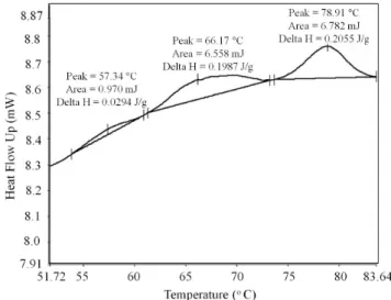
The thermograms obtained were analyzed in the temperature range of 30 °C to 90 °C, using three different software tools: (i)); (ii) OriginPro v.8 (OriginLab Corp., USA); and (iii) Solver tool from MS-Excel (Microsoft Corp., USA). Such software tools were used for estimating the thermal denaturation temperature (Td) of the myosin (TI), sarcoplasmic proteins (TII), and actin (TIII), as well as the value of denaturation enthalpy of these proteins (ΔHI, ΔHII and ΔHIII). Regarding the Pyris 7, the thermal denaturation temperature of the proteins was determined as the maximum temperature of the peaks and the denaturation enthalpy was calculated as the area under the endothermic curve, as shown in Figure 1. In contrast, in the case of the OriginPro software, the denaturation temperature and enthalpy were determined after a peak deconvolution operation. For such a deconvolution procedure, three peak temperatures were estimated (corresponding to the main types of proteins present) and the Gaussian analysis tool provided by OriginPro was used. Konieczny et al. (2016) used the Pyris software to study the DSC thermograms of Anodonta woodiana protein denaturation. However, in order to get deeper insight on the denaturation transition; the authors used the Origin PeakFit module for the deconvolution of the DSC thermograms.
The third software tool used to perform the deconvolution of the peaks, and thus estimate the temperatures and enthalpies of denaturation, was the Solver tool from MS-Excel. For each thermogram obtained by DSC, a least squares methodology was used to make a numerical fit considering a function given by the
sum of three Gaussian functions (Equation 1), corresponding to three major proteins present in the samples (myosin, actin and sarcoplasmic proteins), and a sigmoid function. The Gaussian functions have the form:
2 2 ( ) 2 .exp x b c
y a d
− −
= + (1)
where a is the peak height, b is the temperature (abscissa) of the maximum of the peak, c the parameter that controls the width of the peak, and d the ordinate of the asymptotic limit of the peak’s extremes. A sigmoidal function (Equation 2) was added to the three Gaussian peaks, reflecting a change in the specific heat of the sample during the denaturation transition process:
( ) 1 exp
s x r p
y= − +z
+ (2)
where p is the amplitude of the sigmoid (total ordinate variation),
r is the parameter that controls the gradient of the function, s is the temperature (abscissa) of the inflection point, and z is the ordinate value of the lower branch of the sigmoid.
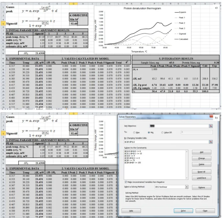
Figure 2a shows the spreadsheet that contains: (i) the experimental data (indicated by “1. Experimental Data”) measured in the DSC calorimeter (time, min; temperature, °C; ∆H, mW); (ii) each of the individually calculated functions (indicated by “2. Values Calculated by the Model”); (iii) the model parameters to be adjusted (“3. Initial Parameters/Adjustment Results”); (iv) the value of the objective function to minimize (“4. Objective Min δ2”); and finally (v) the values of the peak areas which are numerically calculated using the trapezoidal rule (“5. Integration Results”). A plot of the experimental thermogram along with the calculated curve is also included in the spreadsheet aiming to help in finding the initial set of parameters.
In order to prepare the spreadsheet illustrated in Figure 2a for performing the regression, the first step is to “paste” the
data corresponding to experimental observations made by the DSC on the columns in area “1. Experimental Data”. Then, the values of the partial functions and of the respective sum are updated automatically together with the deviations between the experimental and calculated values of the respective squared deviation, appearing in column identified by δ2. The next step is to manually adjust the fitting parameters in area “3. Initial Parameters/ Adjustment Results” in order to adjust the calculated curve as close as possible to the experimental values by properly varying the values of “peak temperature”, “width” and “amplitude”
of each peak. Thus, the manual adjustment of these values must be done based on the experimental data (experimental curve).
After this preparatory phase, the Solver tool accessible from the “Data” tab at the top of the Excel sheet must be is activated, which opens a new window superimposed on the Excel sheet (Figure 2b). In such a window, the conditions/restrictions to be observed during the nonlinear regression process must be specified. The determination of these parameters for the regression is a relatively easy task. Changing some “Options”, accessible through the respective button on the bottom right of the window, may be
necessary and may require some experimentation. To perform the regression calculations, simply press (click) the “Solve” button. After the calculation of the regression, the program asks whether accepting them by choosing “Keep Solver Solution” or rejecting by selecting “Restore Original Values”.
The process can be repeated until there is no change in the sum of the squared deviations. It is important to mention that there are often several local minima, and the solution reached may depend on the initial estimate of the parameters. It is therefore advisable to make several attempts from different “starting points” and, by analyzing the obtained solutions, it becomes possible to identify the best solution (possibly the global minimum). Moreover, it is worth mentioning that the number of attempts can be reduced by using starting points based on the experimental data. The model was prepared for five peaks, but only three are considered by Solver in the example shown. If necessary, all five may be adjusted by Solver.
3 Results and discussion
3.1 Thermograms obtained in DSC analysis
The thermograms of the raw beef and salted beef with different NaCl concentrations (20, 50, 100 and 330 g NaCl L–1 of water) are presented in Figure 3a. In this figure, the formation of three major endotherm peaks was observed. Comparing them with the peaks observed by Brunton et al. (2006) for raw beef, one can infer that they correspond to myosin (± 60 °C), sarcoplasmic proteins (± 65 °C) and actin (78-80 °C). The same authors determined denaturation temperatures of 59 °C for myosin, 66 °C for collagen, and 82 °C for actin.
The thermograms of the samples immersed in brines with different NaCl concentrations are shown in Figure 3a. The increase of NaCl concentration in the brine resulted in a change in the curve profiles with a reduction of peak amplitude, in addition to decrease of the peak temperatures. Kijowski & Mast (1988) also observed a decrease in the endothermic peaks related with myosin and actin for chicken samples when the concentration of the brine was increased from 0 to 40 g NaCl L–1. A similar behavior is reported by Quinn et al. (1980). These authors observed that the thermograms of cured beef samples showed wider peaks, superimposed (less conspicuous) and decreasing peak temperatures with increasing NaCl concentration in the sample of 0.23 M to 0.67 M. This superposition makes it difficult
to determine the denaturation temperature and enthalpy of each protein fraction.
3.2 Temperature and enthalpy of denaturation
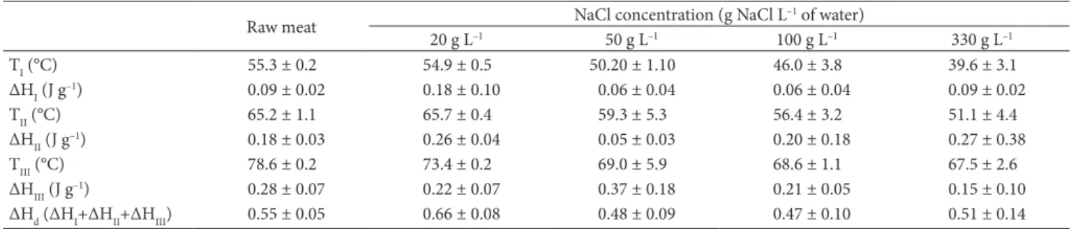
The results of the temperature and enthalpy of denaturation for myosin (TI, ∆HI), sarcoplasmatic proteins (TII, ∆HII) and actin (TIII, ∆HIII) of raw and salted beef samples estimated by the Pyris7 software are presented in Table 1.
Figure 3. Typical DSC thermograms of: (a) raw beef and salted beef with different NaCl concentrations (b) raw beef sample (experimental) with peaks deconvoluted by OriginPro software: myosin (Peak 1), sarcoplasmic proteins (Peak 2), actin (Peak 3) and their sum (calculated).
Table 1. Temperature and enthalpy of denaturation estimated by the Pyris software for proteins of raw beef and salted beef with different NaCl concentration.
Raw meat NaCl concentration (g NaCl L
–1 of water)
20 g L–1 50 g L–1 100 g L–1 330 g L–1
TI (°C) 55.3 ± 0.2 54.9 ± 0.5 50.20 ± 1.10 46.0 ± 3.8 39.6 ± 3.1
ΔHI (J g–1) 0.09 ± 0.02 0.18 ± 0.10 0.06 ± 0.04 0.06 ± 0.04 0.09 ± 0.02
TII (°C) 65.2 ± 1.1 65.7 ± 0.4 59.3 ± 5.3 56.4 ± 3.2 51.1 ± 4.4
ΔHII (J g–1) 0.18 ± 0.03 0.26 ± 0.04 0.05 ± 0.03 0.20 ± 0.18 0.27 ± 0.38
TIII (°C) 78.6 ± 0.2 73.4 ± 0.2 69.0 ± 5.9 68.6 ± 1.1 67.5 ± 2.6
ΔHIII (J g–1) 0.28 ± 0.07 0.22 ± 0.07 0.37 ± 0.18 0.21 ± 0.05 0.15 ± 0.10
As expected, the denaturation temperature of the proteins decreased with the increase of NaCl concentration in the brine, due to the destabilizing effect of the salt on them. The largest variations of denaturation temperature were observed between the raw beef and samples immersed in brine with 330 g L–1. These variations were of 15.7 °C for myosin, 14.1 °C for the sarcoplasmic proteins and 11.1 °C for actin. The value of the sum of denaturation enthalpies (ΔHd = ΔHI + ΔHII + ΔHIII) for the myosin, sarcoplasmic proteins and actin in the raw beef sample was 0.55 J g–1. This value is much lower than that reported by Kazemi et al. (2011) for pork (3.91 J g–1). Such difference can be attributed mainly to the different methods used to calculate ΔHd. For instance, in the case of the method implemented in the Pyris software, the start and the end of the peak must be marked manually and the enthalpy is calculated from the area under straight line that connects the start and the end of the peak. This procedure ignores a significant portion of the area and may thus result in lower enthalpy.
Regarding the total enthalpy of denaturation (ΔHd) of the protein, a gradual decrease with increasing NaCl concentration was not observed, contrasting with the results reported by Kijowski & Mast (1988).
As previously mentioned, the reduction of peak amplitude, as well as the possible overlapping of the peaks, may hamper the determination of the temperature and enthalpy of denaturation. To obtain more reliable results, the deconvolution of the thermogram’s peaks was performed using both the OriginPro software and a procedure developed in MS-Excel. Figure 3b shows the deconvolved thermogram of raw beef sample obtained using the Gaussian analysis tool of the OriginPro software. The calculated curve is related to the sum of the three individual peaks corresponding to each protein.
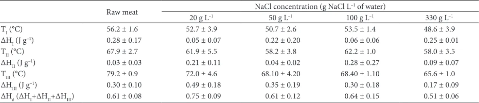
The values of denaturation temperature and denaturation enthalpy of the different proteins are presented in Table 2. These values were estimated by deconvolution of the thermograms of raw and salted beef samples using OriginPro software.
A smaller variation of denaturation temperature of myosin and sarcoplasmic proteins was observed between the raw samples and the immersed in brine with 330 g L–1 when compared with the temperatures obtained by the Pyris software. The variation of temperatures using OriginPro software was 7.6 °C for myosin, 9.9 °C for the sarcoplasmic proteins and 13.6 °C for actin. Graiver et al. (2006) also observed a greater variation in
denaturation temperature of actin (∆T = 13 °C) than for myosin (∆T = 4 °C), when the level of NaCl increased up to 50 g L–1. The value of the sum of denaturation enthalpies (ΔHd) of the myosin, sarcoplasmic proteins and actin estimated by OriginPro in the raw meat sample (0.61 J g–1) is lower than that reported by Kazemi et al. (2011) for pork (3.91 J g–1).
The same experimental data used to determine temperatures and enthalpies of denaturation of beef samples using Pyris and OriginPro software were also used in the procedure developed for the MS-Excel. The result obtained using this procedure for the deconvolution of the thermogram of the raw beef sample is presented in Figure 4.
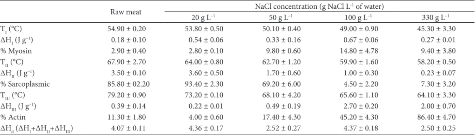
The values determined by the deconvolution of peaks using MS-Excel for denaturation temperature and enthalpy as well as the percent of each protein (myosin, actin and sarcoplasmic) present in the samples are presented in Table 3. The results show that denaturation temperature decreased with increasing NaCl concentration in the brine. The change of calculated denaturation temperature between the raw samples and those immersed in brine with 330 g L–1 was 9.6 °C for myosin, 9.7 °C for the sarcoplasmic proteins and collagen, and 15.1 °C for actin. These results (estimated by the model) are consistent with those found by Graiver et al. (2006), which points out that the increase of NaCl concentration has a greater influence on the denaturation temperature of actin. Moreover, the calculated value for total denaturation enthalpy (ΔHd) of the raw sample estimated by the model (4.07 J g–1) has a better agreement with that found by Kazemi et al. (2011) in raw pork (3.91 J g–1) than the value estimated by the Pyris and OriginPro software. Still concerning the value of total denaturation enthalpy, as expected, a decrease was observed between raw samples and those immersed in brine with 330 g L–1 (from 4.07 J g–1 to 2.50 J g–1).
The smallest values of denaturation temperature of beef protein determined using the different software tools ranged from 39.6 to 48.6 °C. Such a variation of approximately 10 °C can be considered high, especially in applications where the temperature is a critical parameter to be controlled to avoid undesirable changes in the product structure (for instance, in drying processes). This demonstrates the importance of the choice of the methodology for deconvolution of the thermograms. Based on the results obtained for denaturation temperature and denaturation enthalpy of each protein, one can conclude that the model developed and programmed in MS-Excel showed better
Table 2.Temperature and enthalpy of denaturation estimated by the OringinPro software for proteins of raw beef and salted beef with different NaCl concentration.
Raw meat NaCl concentration (g NaCl L
–1 of water)
20 g L–1 50 g L–1 100 g L–1 330 g L–1
TI (°C) 56.2 ± 1.6 52.7 ± 3.9 50.7 ± 2.6 53.5 ± 1.4 48.6 ± 3.9
ΔHI (J g–1) 0.28 ± 0.17 0.05 ± 0.07 0.22 ± 0.20 0.06 ± 0.06 0.25 ± 0.01
TII (°C) 67.9 ± 2.7 61.9 ± 5.5 58.2 ± 3.8 62.2 ± 1.0 58.0 ± 3.5
ΔHII (J g–1) 0.03 ± 0.03 0.21 ± 0.11 0.04 ± 0.02 0.28 ± 0.27 0.09 ± 0.07
TIII (°C) 79.2 ± 0.9 72.0 ± 4.6 68.10 ± 4.20 68.40 ± 1.10 65.6 ± 1.0
ΔHIII (J g–1) 0.30 ± 0.10 0.49 ± 0.18 0.35 ± 0.19 0.30 ± 0.18 0.17 ± 0.09
increase of NaCl concentration in the beef samples. The presented methodology, based on the use of MS-Excel and the Solver tool, was capable of estimating the peak temperatures and the contribution of each protein for the denaturation enthalpy in raw samples and samples immersed in brine with different NaCl concentrations. It is important to mention that the proposed calculation procedure may be easily adapted to the analysis of other overlapping spectra, containing peaks that can be described by Gaussian functions.
Acknowledgements
The authors thank to CAPES/Brazil and CNPq/Brazil for financial support.
agreement with the data found in literature than the results obtained with the Pyris and OriginPro tools.
4 Conclusions
This paper presents contributions to the estimation of denaturation temperature of beef proteins, which is of special interest for the development of industrial procedures. Moreover, this paper illustrates the application of widely available software tools for the deconvolution of DSC thermograms of beef protein denaturation. The peak deconvolution procedure facilitates the estimation of the values of the denaturation temperature and enthalpy, resulting in more consistent values. The obtained results indicate that, regardless of the software tool used, the denaturation temperature of the proteins decreased with the
Figure 4. Thermogram of raw beef sample (experimental) with peaks deconvoluted by MS-Excel Solver tool: myosin (Peak 1), sarcoplasmic proteins (Peak 2), actin (Peak3) and their sum (calculated).
Table 3. Temperature and enthalpy of denaturation estimated by the MS-Excel Solver tool for proteins of raw beef and salted beef with different NaCl concentration.
Raw meat NaCl concentration (g NaCl L
-1 of water)
20 g L–1 50 g L–1 100 g L–1 330 g L–1
TI (°C) 54.90 ± 0.20 53.80 ± 0.50 50.10 ± 0.40 49.00 ± 0.90 45.30 ± 3.30
ΔHI (J g–1) 0.18 ± 0.10 0.54 ± 0.06 0.33 ± 0.16 0.67 ± 0.06 0.27 ± 0.01
% Myosin 2.90 ± 0.40 2.80 ± 0.10 9.80 ± 0.60 14.80 ± 4.78 9.40 ± 3.80
TII (°C) 67.90 ± 2.70 64.00 ± 0.80 62.70 ± 1.20 59.90 ± 1.60 58.20 ± 0.50
ΔHII (J g–1) 3.50 ± 0.10 3.60 ± 0.50 1.70 ± 0.60 1.00 ± 0.30 0.23 ± 0.07
% Sarcoplasmic 85.80 ± 02.20 93.40 ± 2.30 69.20 ± 6.00 4.50 ± 2.20 7.30 ± 3.20
TIII (°C) 79.20 ± 0.90 73.20 ± 0.10 68.10 ± 4.20 65.60 ± 1.10 64.10 ± 3.30
ΔHIII (J g–1) 0.39 ± 0.14 0.22 ± 0.01 0.49 ± 0.19 2.70 ± 0.20 2.00 ± 0.70
% Actin 11.30 ± 1.80 4.00 ± 0.60 17.40 ± 4.30 45.20 ± 4.30 86.40 ± 4.70
Konieczny, P., Tomaszewska-Gras, J., Andrzejewski, W., Mikołajczak, B., Urbanska, M., Mazurkiewicz, J., & Stangierski, J. (2016). DSC
and electrophoretic studies on protein denaturation of Anodonta
woodiana (Lea, 1834). Journal of Thermal Analysis and Calorimetry,
126(1), 69-75. http://dx.doi.org/10.1007/s10973-016-5707-0. Quinn, J. R., Raymond, D. P. R. A., & Harwalkar, V. R. (1980). Differential
scanning calorimetry of meat proteins as affected by processing
treatment. Journal of Food Science, 45(5), 1146-1149. http://dx.doi.
org/10.1111/j.1365-2621.1980.tb06507.x.
Thorarinsdottir, K. A., Arason, S., Geirsdottir, M., Bogason, S. G., & Kristbergsson, K. (2002). Changes in myofibrillar proteins during processing of salted cod (Gadusmorhua) as determined by
electrophoresis and differential scanning calorimetry. Food Chemistry,
77(3), 377-385. http://dx.doi.org/10.1016/S0308-8146(01)00349-1. Toledo-Núñez, C., Vera-Robles, L. I., Arroyo-Maya, I. J., &
Hernández-Arana, A. (2016). Deconvolution of complex differential scanning calorimetry profiles for protein transitions under kinetic control.
Analytical Biochemistry, 509, 104-110. PMid:27402175. http://dx.doi.
org/10.1016/j.ab.2016.07.006.
Vega, S., Garcia-Gonzalez, M. A., Lanas, A., Velazquez-Camp Raymond oy, A., & Abian, O. (2015). Deconvolution analysis for classifying gastric adenocarcinoma patients based on differential scanning calorimetry
serum thermograms. Scientific Reports, 5, 1-8. PMid:25614381.
http://dx.doi.org/10.1038/srep07988.
References
Albarracín, W., Sánchez, I. C., Grau, R., & Barat, J. M. (2011). Salt
in food processing; usage and reduction: a review. International
Journal of Food Science & Technology, 46(7), 1329-1336. http://
dx.doi.org/10.1111/j.1365-2621.2010.02492.x.
Brunton, N. P., Lyng, J. G., Zhang, L., & Jacquier, J. C. (2006). The use of dielectric properties and other physical analyses for assessing protein denaturation in beef biceps femoris muscle during cooking
from 5 to 85 °C. Meat Science, 72(2), 236-244. PMid:22061550.
http://dx.doi.org/10.1016/j.meatsci.2005.07.007.
Furukawa, V. A., Sobral, P. J. A., Habitante, A. M. Q. B., & Gomes, J. D.
F. (2004). Análise térmica da carne de coelhos. Ciência e Tecnologia
de Alimentos, 24(2), 265-269.
http://dx.doi.org/10.1590/S0101-20612004000200018.
Graiver, N., Pinotti, A., Califano, A., & Zaritzky, N. (2006). Diffusion
of sodium chloride in pork tissue. Journal of Food Engineering,
77(4), 910-918. http://dx.doi.org/10.1016/j.jfoodeng.2005.08.018. Kazemi, S., Ngadi, M. O., & Gariépy, C. (2011). Protein denaturation
in pork longissimus muscle of different quality groups. Food
Bioprocess Technology, 4(1), 102-106. http://dx.doi.org/10.1007/
s11947-009-0201-3.
Kijowski, M., & Mast, M. G. (1988). Effect of sodium chloride and phosphates
on the thermal properties of chicken meat proteins. Journal of Food
Science, 53(2), 67-387. http://dx.doi.org/10.1111/j.1365-2621.1988.