Numerical experiments with the Generalized Finite Element Method based on a flat-top Partition of Unity

Numerical experiments with the Generalized Finite Element Method

based on a flat-top Partition of Unity

Abstract

The Stable Generalized Finite Element Method SGFEM is essentially an improved version of the Generalized Finite Element Method GFEM . Besides of retaining the good flexibility for constructing local enriched approximations, the SGFEM has the advantage of presenting much better conditioning than that of the conventional GFEM. Actually, bad conditioning is well known as one of the main drawbacks of the GFEM, while affecting severely the precision of the numerical scheme used for solving the linear system associated to the problem. Despite of its consistent mathematical basis, the numerical experiments so far conducted on using SGFEM are not yet clearly conclusive, especially regarding the robustness of the method. Therefore, the main purpose of the present paper is to give a contribution in this direction, through further investigating the SGFEM accuracy and stability. In particular, the so called Flat-Top SGFEM is a recent proposed version of the method hereby considered. As a flat-top Partition of Unit PoU is used for constructing the augmented approximation space with polynomial enrichments this version of the method is called SGFEM with flat-top PoU, or simply FT-SGFEM. Some computational aspects are briefly addressed, as the ones related to the implementation and integration of the flat-top for 2-D analysis. The numerical simulations consist essentially of linear analysis of panels presenting edge cracks and reentrant corners on its boundaries. Our findings from the numerical tests done are highly relevant regarding accuracy of the SGFEM versions, which present order of convergence similar to the conventional GFEM. Moreover, the measure of stability given by the scaled condition number presented in particular by the FT-SGFEM is comparable to the conventional FEM order.

Keywords: Generalized Finite Element Method. Flat-top Stable Generalized Finite Element Method. h-convergence. Scaled condition number.

1 INTRODUCTION

The Generalized Finite Element Method GFEM is a Partition of Unity PoU based Galerkin method, according to which the basic approximation space provided by a PoU is enlarged by shape functions constructed trough the product of the PoU by functions with good approximation skills, referred to as enrichment functions. The key concept behind such procedure is that the product of the PoU functions with any given enrichment function can exactly reproduce it. In fact, this concept was primarily introduced in the Partition of Unity Method

PUM framework, Melenk and Babuška 1996 .

The GFEM and the eXtended Finite Element Method XFEM , Belytschko et al. 2009 , are both PoU based methods sharing the same fundamentals. In particular, a mesh of finite elements is used to provide a PoU, which is commonly defined through the piecewise linear Lagrangian shape functions embodied in the elements. Owing to such special feature and also considering that the unity is always taken as the first component of the set of enrichment functions, the GFEM/XFEM can also be understood as an extension of the conventional Finite Element Method FEM for which the local approximations provided by the shape functions are enlarged by means of enrichment functions.

The GFEM/XFEM enrichment framework, while dispensing with costly mesh refinements, has proved to be efficient in a variety of applications, mainly when the solution’s local behavior is of major interest and, therefore, must be properly reproduced. Problems of the Linear Fracture Mechanics likely are among the most benefited by

Fernando Massami Satoa* Dorival Piedade Netoa

Sergio Persival Baroncini Proençaa

a_{Universidade de São Paulo – USP, São Carlos,}

São Paulo, Brasil. E-mail: fernandomsato@gmail.com,

dpiedade@sc.usp.br, persival@sc.usp.br * Corresponding Author

http://dx.doi.org/10.1590/1679-78254222

Received: July 07, 2017

the method. For instance, crack tip stress concentrations are better mimicked through branch functions enrichment of the approximation imposed at patches nearby the tip, as suggested for instance in Oden and Duarte 1997 , Belytschko and Black 1999 , Moës et al. 1999 , Duarte et al. 2001 , Pereira et al. 2009 , Sukumar et al. 2000 and Sukumar et al. 2003 . Furthermore, mesoscale cracking modeling of polycrystalline materials, as well as modeling of solids containing interfaces, voids and inclusions, see Simone et al. 2006 and Alfaiate et al. 2003 , are further classes of problems in which the GFEM/XFEM features are advantageous with respect to conventional FEM modeling.

Even though the GFEM is being successfully applied to solve a wide class of mechanical problems, an improper choice of the enrichment functions can cause bad conditioning of the global stiffness matrix, therefore affecting severely the precision of the numerical scheme used for solving the linear system associated to the discretized weak form of the problem. So, the conditioning of the GFEM could be much worse than that of the standard FEM and, ultimately, have a deleterious effect on the robustness of the method.

The Stable Generalized Finite Element Method SGFEM , Babuška and Banerjee 2011 , is essentially an improved version of the GFEM and was conceived to overcome the conditioning issue. In effect, besides of retaining the good flexibility for constructing local enriched approximations, the main advantage of the SGFEM is to present a much better conditioning than that of the conventional GFEM. Despite of its consistent mathematical basis, the numerical experiments so far conducted on using SGFEM are not yet clearly conclusive, especially regarding the robustness of the method. Therefore, the method still demands further practical investigation on the accuracy and stability properties compared to the standard GFEM and also to the conventional FEM approaches.

The main purpose of the present paper is to give a contribution concerning the investigation of the SGFEM accuracy and stability by means of computational experiments. In particular, the recent proposed version of the method, called higher order SGFEM, is hereby considered, Zhang et al. 2014 . In line with this reference only second degrees complete and incomplete shifted polynomial functions are used as enrichment of the approximation. Moreover, a ‘flat-top’ PoU function is used for constructing the enrichment part of the augmented approximation space instead of the usual piecewise linear hat functions, Sato 2017 , that are still preserved for the basic part of the approximation space. In order to highlight such particular feature, the SGFEM with flat-top PoU, or simply FT-SGFEM, is hereby referenced instead of the higher order SGFEM.

Some computational aspects are briefly addressed, as the ones related to the implementation and integration of a flat-top partition of unit locally at the element level. The problems considered for the computational experiments hereby reported consist of two-dimensional linear analysis of panels presenting edge cracks and reentrant corners. Actually, these problems are typically useful to demonstrate the efficacy of the GFEM for exploring special enrichments. However, as already mentioned only polynomial enrichments are considered, since the good conditioning provided by the use of the flat-top PoU is the main concern hereby emphasized.

Our findings from the computational experiments done are highly relevant while confirming the favorable features of good conditioning and order of convergence, which can be proved analytically, Zhang et al. 2014 , once certain assumptions on the augmented approximation space are satisfied. In particular, regarding the issue of numerical stability the resulting scaled condition numbers similar to the ones exhibited by the conventional FEM indicate the advantage of the FT-SGFEM compared to the standard GFEM.

The remaining of the paper is organized in the following way. In Section 2, the weak form of the Boundary Value Problem BVP is addressed followed by an introduction on the GFEM and SGFEM main features. In section 3 the SGFEM with a flat-top PoU is described. Next, some computational aspects are briefly emphasized, as the ones related to the implementation and integration of a flat-top partition of unit for constructing the augmented approximation space with polynomial enrichments. In section 4, the results of the computational experiments selected for analysis are shown. Finally, in Section 5, some important conclusions on the accuracy and numerical conditioning provided by the SGFEM using flat-top PoU are emphasized.

2 THE WEAK FORM OF THE BOUNDARY VALUE PROBLEM BVP

The weak statement of the static equilibrium problem of a linear elastic solid is hereby provided in a Galerkin approach by the Principle of Virtual Work, which reads: find the small displacement field

u



V

t such that for

u V



:

N

s s

u



u d

f u d



t u d

















 



 













1

where

V

t is the standard space of trial functions for the elasticity problem and V the space of test functions,

respectively defined as

 



1

_:

_{( , )}



t D

V



u



H



u



u X t

for X on



2

 



1

₀



V



w



H



: w



for X on



_D 3

In the relations above Ω denotes the domain occupied by the body, with boundary

  

N





Dand N D



_

  

.



N and



Ddenote the Neumann and Dirichlet boundaries, respectively. u is the virtual

displacement vector from the equilibrium position,



s

 

.

is the symmetric part of the gradient operator used to construct both compatible strain and virtual strain second order tensors,



is the linear elastic rigidity tensor of fourth order,

f

is the body forces vector and t is the vector of prescribed tractions at the static part Neumann of the solid’s boundary.

The Finite Element Method FEM provides a discretization for the weak form of the BVP through a strategy for defining trial/test approximations for the displacement fields involved. At the element level an approximation is constructed by a linear combination of

n

_ nodal element shape functions e





taking as parameters the nodal values

_u

e

 of the trial displacement field, as follows:

( )

n

( )

e e e

u x

x u



 









4

Basically, as shown on what follows, the main difference between the standard FEM and the GFEM is in the definition of the element shape functions.

2.1 The GFEM local and global approximations

To comprise the possibility that the solution can change from one part to another of the domain, in the GFEM the approximation is constructed into subdomains called patches. A mesh of finite elements linking N nodes and discretizing the solid domain is used for defining the nodal patches. The gain of approximation is achieved through augmenting the basic FEM approximation space by exploring the concept of Partition of Unity PoU for constructing the local enriched approximations. A variety of PoU can be used, however in the GFEM the PoU is directly supplied by the FEM mesh. Often piecewise linear ‘hat’ functions provided by the triangular finite element mesh or bilinear functions provided by quadrilateral elements are commonly explored as PoU for 2-D analysis purposes. One important characteristic of the GFEM is that the underlying mesh keeps unchanged.

As already mentioned before, the shape functions



i are defined locally in a domain called nodal patch

set of elements having a common node as vertex . Inside of each patch α , the shape functions are constructed by the product between the so-called enrichment functions

L

i and the partition of unity functions belonging to

the elements in the patch and attached to the vertex. Therefore, the shape functions for the GFEM are written as:

i

L

i

  







5

where







1, ,



N



_{identifies the nodal patch and}

i



1, ,



ne

 



_{identifies the enrichment function}

ne

 



is the total number of enrichment functions adopted for the patch . In the GFEM, normally the first component of the enrichment functions set is assumed as equal to the unity, i.e.

L

1



1

. Therefore, the FEM approach always

belongs to the approximation space of the GFEM.

certain complete polynomial degree is hereby used. Accordingly, the general form of the polynomial enrichment component basis can be expressed by the shifted arrangement as follows



 



( , )

m n

m n

X X Y Y

L m n

h       6

where Xα and Yα are the coordinates of the patch vertex node α and h is a scaling factor given, for instance, by the radius of the circle centered at the vertex and circumscribing the largest element of the patch. One of the most remarkable advantages of the shifted enrichment functions is that they are zero in the node where they are imposed. It follows that the physical significance of the original degree of freedom associated to the basic part of the approximation at such a node is preserved. Moreover, this feature enables one, in principle, to directly enforce displacement boundary conditions in the same way as in the FEM.

As a rule, in 2-D analysis the enrichment functions are common to both displacement components. Once the enriched approximations are set in each patch a partition of unity is used to paste the local approximations together forming a global regular approximation. Therefore, by restricting only to 2-D problems, the GFEM global approximation for each component of the displacement field is given by the following relations:

1 1 2

ˆ

N N nl i i

i

u

_{ }

u

_{ }

b

 





  



_



_

7

1 1 2

ˆ

N N nl i i

i

v

_{ }

v

_{ }

c

 





  



_



_

8

where

u

_{ and}

v

_{are parameters associated with usual degrees of freedom of the FEM,}

b

_iand

c

_{iare additional}

nodal parameters introduced by enrichment. In the previous relations a convenient splitting of the GFEM approximation space is explored, putting in evidence the basic part provided by the FEM and the enrichment part. Therefore, being S1 the basic space and S2 the enrichment space, formally the GFEM approximation space

SGFEM can be represented as follows:

1 2

GFEM

S

 

S

S

9 1 1 1 2 1 2

:

:

N N nl i i i

S

a

S

L a

      

 



 



  







_



_











_



_







 

10 Once trial/test functions given by the approximation space are inserted in the Principle of Virtual Work relation, the resulting discretized weak form provides the specific values for the set of nodal parameters, therefore associating the finite dimensional global approximation to the exact solution of the BVP.

Of course, the accuracy of the global approximate solution depends on the favorable properties of the local approximation spaces. In this regard, there are no restrictions to the type and number of enrichment functions to be attached to a given node. Hence, the number of degrees of freedom is totally flexible. Consequently, at the element level, the size of the resulting element stiffness matrix may change drastically, depending on the adopted enrichment scheme. Moreover, once a Galerkin approach is used, the element equivalent forces vectors also present variable sizes.

Notwithstanding the favorable aspects mentioned above, the polynomial enrichment approach may introduce linear dependencies in the resulting system of equations, therefore affecting the numerical stability and accuracy of the method. This kind of issue is well-known as one of the most significant drawbacks of the GFEM. However, as shown in this work, once certain assumptions are satisfied for constructing the shape functions the polynomial enrichment approach can be explored efficiently.

2.2 The SGFEM local and global approximations

More precisely, the enrichment functions for a patch α are constructed by the difference between the original enrichment function

L

i and the piecewise linear or bilinear finite element interpolant function of it

I

_ . Therefore,

 

mod

i i i

L

L

I

L











  11

At the element level the interpolant function can be written as:





1

,

n

j i j j j

I

L

X Y















_

12

where

X Y

j

,

j are the coordinates of node j of the element in question.

The conventional procedure for constructing the GFEM shape functions is then used to define the SGFEM shape functions



modi . Hence,

mod mod

i

L

i

  







13

Thus, it is convenient to represent the SGFEM approximation space as follows:

mod

1 2

SGFEM

S

 

S

S

14

  1 1 1 mod mod 2 1 2

:

:

N nl N i i i

S

a

S

L

a

       

 



 



  







_



_











_



_







 

15

The interpolant function and the resulting shape function considered in SGFEM are highlighted in Figure 1.

Figure 1: Construction of an enrichment function and a shape function used in SGFEM, adapted from Figure 2 of Gupta et al. 2013 .

3 THE SGFEM WITH FLAT-TOP PARTITION OF UNITY

As proposed in Zhang et al. 2014 , the higher order SGFEM yields higher order convergence and presents good conditioning derived from a further specific modification of the enrichment space, which is simple enough for retaining the good flexibility for constructing local enriched approximations as in the standard SGFEM.

Such an additional modification aims to guarantee that the shape functions of the enriched space be locally linearly independent. Essentially, the procedure hereby adopted consists of using another PoU for constructing the

S

2modspace, different from the piecewise hat functions that however are preserved for constructing the basic S1 space. Thus, the SGFEM with ‘flat-top’ PoU approximation space is represented as follows:

mod

1 2

SGFEM

S

 

S

S

16

  1 1 1 mod mod 2 1 2

:

:

N nl N i i i

S

a

S

N

L

a

       

 



 

  







_



_











_



_











17

In the mod 2

S

space definition,

L

mod_i is constructed just as indicated in relation 11 , while

N

_ represents the so called flat-top function, Sato 2017 , hereby adopted as PoU.

The flat-top function can be constructed element-wise. In 1-D it can be easily defined by considering a unitary domain,

 

(0,1)

discretized by N nodes equally spaced. If h is the distance between a pair of nodes, then the nodal coordinates are given by:



x

i



ih



Ni₀. For a parameter 0 0.5 and a positive integer l, the

element-wise flat-top PoU is defined as follows:

 

_

_









1

1

,

1

,

1

1 2

0

1

,

j j l

l j

Left j j

j j

x

x x

h

x

x

h

N

x

x

x

h x

h

h

x

x

h x















_







_





_



 

_

_{ }

_



 









_



_

_

_

_



_



 

_



_



_



 











 



_

_



18

 

_

_









1

0

,

1 1

,

1

1 2

1

1

,

j j l

l j

Right j j

j j

x

x x

h

x

x

h

N

x

x

x

h x

h

h

x

x

h x















_







_





_





_

_

_{ }

_

_



_

_

_

_





 

_



_

_



_

_



_



 

_







_

_









 



_

_



19

In the relations above, x is a local coordinate with origin at the left node of the element xj ,

N

Left

 

x

 _{is for}

the PoU component attached to the node xj and

N

Right

 

x



is the PoU component attached to node xj 1.

Figure 2: Flat-top partition of unity, 1-D and 2-D illustrations

To deal with the numerical integration of the stiffness matrix components as well of the equivalent nodal forces vector with flat-top functions, an appropriate strategy is hereby conceived, Sato 2017 . Therefore, subdomains are attributed in agreement with the piecewise definition of the flat-top function inside the element. Then, standard quadrature integration rules are applied in each subdomain.

Accordingly, four characteristics subdomains of the flat-top PoU component can be revealed when considering the master element domain, as shown in Figure 3 a , each one being expressed by a polynomial function. The areas 1 and 4 have constant values 1 and 0 respectively, the areas 2 are described by a ‘ramp’ function, and the area 3 is described by a higher order polynomial function.

Therefore, the element can be split in nine parts, as shown in Figure 3 b , next applying the Gauss quadrature rule to each subdomain for computing the components of the stiffness matrix and equivalent nodal force vector. Moreover, the numerical integration encompasses only the regions 1 to 3. Essentially, this is the strategy hereby adopted for generating the results of the examples presented later on.

The implementations were done using a Python based computational code for the GFEM following the object-oriented programing paradigm, described in Piedade Neto et al. 2013 .

4 NUMERICAL EXAMPLES

In what follows, two numerical examples are presented. In each of them, only structured meshes and enrichment schemes with shifted polynomial functions were investigated.

The first example is an L-shaped panel. The main aim is to verify accuracy of results in displacements and stress provided by the SGFEM with flat-top PoU. Moreover, convergence order and scaled condition number are presented by confronting the results of the standard GFEM and SGFEM.

The second example aims to illustrate the potential of the GFEM versions even if a crack is included at one edge of a panel. Again, the accuracy and stability of the method are shown through the analysis of the convergence order and scaled condition number.

Despite of local non-smoothness implicit in both examples, it is shown that the method provides asymptotic convergence with mesh refinement.

4.1 L-shaped panel

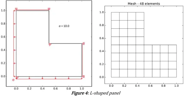
The first example consists of an L-shaped panel under uniform distributed loading at the longer edges, as depicted in Figure 4. Sliding supports are prescribed at the Dirichlet’s boundaries. The material has a linear elastic response, being adopted Young’s Modulus of 100 and Poisson’s ratio of 0.3 as elastic parameters. Moreover, unitary thickness and plane stress conditions are assumed.

Six structured meshes varying from coarse to fine and composed by bilinear quadrilateral elements are used in this case. These meshes present the following grid sizes, indicated according to the number of elements in the longer and shorter edges, respectively as: 4 X 2 , 8 X 4 , 16 X 8 , 32 X 16 , 64 X 32 and 128 X 64 .

Figure 4: L-shaped panel

In this example, a comparison between the GFEM versions is presented. The main aspects evaluated are rate of convergence based on the estimate errors on displacements and scaled condition number.

The relative error on displacements is computed using the L2 norm as follows:

2

2

ref _L ref _L

u

u

relative error

u







20

In the relation above, uref is for the reference solution computed by FEM using a very refined mesh 2048 X 1024 and ũ is for the approximate solution.

Firstly, since the split strategy of numerical integration described in the last section is adopted for the SGFEM with flat-top PoU, values for



between limits 0 and 0.5, as well the number of integration points can be chosen arbitrarily. Therefore, a preliminary study considering different values of



is presented next to verify its efficacy.

The analysis of the results is made by confronting the convergence rates of relative error on displacements for



values equal to 0.1, 0.2, 0.3 and 0.4.

Another important measure to compare is the scaled condition number SCN . Following Babuška and Banerjee 2011 , this value is given by the ratio between the highest and the lower eigenvalues of the scaled stiffness matrix of the linear system associated to the GFEM version chosen. Representing by K the stiffness matrix, the scaled one is defined as:

ˆ

K



D K D

₂₁

where D is a diagonal matrix in which the diagonal terms are computed as:

D

ii

K

ii1/ 2 



.

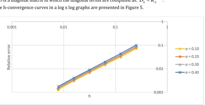
The h-convergence curves in a log x log graphs are presented in Figure 5.

Figure 5: L-shaped panel: h-convergence for different values of



It can be concluded that the lower the



value is, the better the solution becomes. Actually, by strongly decreasing the



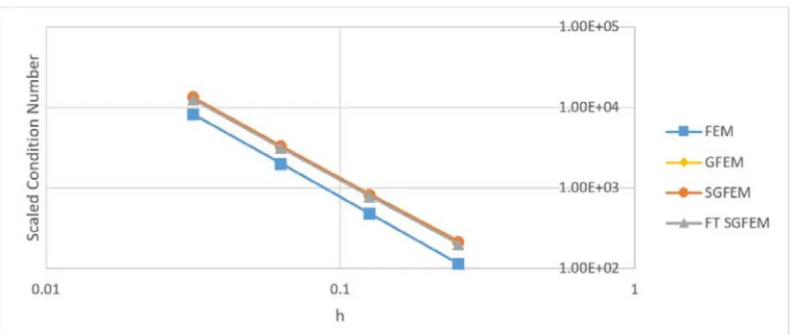
value, the flat-top approaches to the hat-function PoU. Consequently, the FT-SGFEM turns into the SGFEM.

On the opposite sense, the scaled condition number increases once the complete polynomial enrichment is used. To illustrate such an effect, the SCN is presented in Figure 6. It can be seen that there is practically no difference when comparing the SCN values for different parameters



adopted, therefore the h-convergence curves result practically coincident. Moreover, the SCN values are of order h-2_{, i.e., for h decreasing of one order}

Figure 6: L-shaped panel: scaled condition number for



analysis

In conclusion, since





0 1

.

_{was shown to have the lowest value of relative error, this value will be selected}

for the next analyses.

The relative errors obtained for the case of incomplete enrichment are reported in Table 1.

Table 1: L-shaped panel. Relative error for incomplete polynomial

Mesh h FEM GFEM SGFEM FT SGFEM _{ 0.1}

4x2 0.25 0.1423 0.08988 0.07063 0.078560718

8x4 0.125 0.06743 0.03542 0.032 0.034963031

16x8 0.0625 0.03046 0.01567 0.01483 0.016122405

32x16 0.03125 0.0137 0.00711 0.00682 0.007415862

64x32 0.01563 0.00615 0.00318 0.00306 0.003339863

128x64 0.00781 0.00271 0.00135 0.0013 0.001429723

The log x log graphs depicted in Figure 7 show the h-convergence of the relative error for the case of incomplete enrichment. It must be pointed out that this is not a regular problem, once the reentrant corner of the L-shaped panel induces stress singularity. Even so, it can be observed that comparing GFEM and SGFEM versions to the FEM, the convergence rates are pretty much of the same order.

In terms of comparative gains, the relative errors provided by the GFEM versions are very close in values to the ones obtained through FEM, however, demanding a mesh one level coarser. Therefore, when analyzing the number of degrees of freedom involved in this example, the GFEM versions have spent less DoF for obtaining the same relative error, as shown in Table 2. Of course, such reduction in the DoF implies in a low processing time.

Table 2: L-shaped panel. Degrees of freedom for incomplete polynomial

Mesh h FEM GFEM/SGFEM

4x2 0.25 42 126

8x4 0.125 130 390

16x8 0.0625 450 1350

32x16 0.03125 1666 4998

64x32 0.01563 6402 19206

128x64 0.00781 25090 75270

The Figure 8 shows the SCN for the methods using the incomplete enrichment. It is observed that the values obtained for the GFEM versions are close to the FEM values. Moreover, the SGFEM versions do not present any advantage over the GFEM, since the incomplete enrichment verifies the linear independence condition already for the GFEM.

Figure 8: L-shaped panel. Scaled condition number for incomplete polynomial

However, as reported in Table 3, when a complete enrichment is considered, the SCN is strongly affected in the SGFEM, which remains comparable to the bad condition level shown by GFEM. This is evidence that the resulting enriched space lacks of linear independence property. On the other hand, linear independence property is recovered by the enrichment space when using flat-top PoU. Such good advantage is well marked in Table 3 by the corresponding dropping of the SCN values comparable to the level presented by the FEM ones.

Table 3: L-shaped panel. Scaled condition number for complete polynomial

Mesh h FEM GFEM SGFEM FT SGFEM _{ 0.1}

4 x 2 0.25 2.16E 02 3.87556E 16 4.00E 16 4.02E 02

8 x 4 0.125 9.43E 02 1.37449E 17 2.19E 15 1.59E 03

16 x 8 0.0625 3.87E 03 1.69705E 17 8.10E 15 6.34E 03

Although the employment of the flat-top PoU results in a well-conditioned matrix, as consequence of its limited capacity of approximation, the relative error is a little higher than that obtained through SGFEM. Despite of that, the SGFEM using flat-top PoU benefits from the mesh refinement.

However, in face of results, as the FT-SGFEM with complete quadratic polynomials and the SGFEM with an incomplete set both provide good condition numbers and accuracy, it is interesting to compare their plots. This is precisely what is shown in Figure 9.

Figure 9: Effect of mesh refinement for the incomplete SGFEM above and complete FT-SGFEM below

4.2 Panel with an edge crack

The selected problem for analysis is presented in Figure 10.

Sliding supports are prescribed at the Dirichlet’s boundaries. The material has a linear elastic response, being adopted Young’s Modulus of 100 and Poisson’s ratio of 0.3 as elastic parameters. Moreover, unitary thickness and plane stress conditions are assumed.

Six structured meshes varying from coarse to fine and composed by bilinear quadrilateral elements are used in this case. These meshes present the following grid sizes, indicated according to the number of elements in the horizontal and vertical directions, respectively as: 4 X 4 , 8 X 8 , 16 X 16 , 32 X 32 , 64 X 64 and 128 X 128 .

Analogous to the previous example, shifted complete and incomplete second degree polynomial options of enrichment are considered and applied to the whole set of nodes. Again, a comparison between GFEM versions is presented. The main aspects evaluated are rate of convergence based on the estimate errors on displacements and scaled condition number. In particular a reference solution was computed by FEM using a very refined mesh

2048 X 2048 .

The relative errors on displacements computed using the L2 norm for the case of incomplete enrichment are reported in Table 4.

Table 4: Edge cracked panel. Relative errors for incomplete polynomial enrichment

Mesh h FEM GFEM SGFEM FT SGFEM  0 1.

4x4 0.25 0.26134 0.17022 0.15184 0.166581834

8x8 0.125 0.14344 0.08548 0.08275 0.089600582

16x16 0.0625 0.07421 0.04378 0.04392 0.047327711

32x32 0.03125 0.03741 0.02209 0.02247 0.024203718

64x64 0.01563 0.01853 0.01088 0.01113 0.012011457

128x128 0.00781 0.00898 0.00515 0.0053 0.005740655

The log x log graphs depicted in Figure 11 show the h-convergence of the relative errors. Even if this is not a regular problem, as the crack tip induces heavy stress singularity, it can be observed that the convergence rates are pretty much of the same order comparing GFEM versions with FEM.

Figure 11: Edge cracked panel: relative error values for incomplete polynomial and mesh refinement

Figure 12: Edge cracked panel: scaled condition number for incomplete polynomial and mesh refinement

However, when considering complete second degree polynomial enrichment, the SCN for SGFEM is strongly affected, becoming comparable to the bad condition level shown by GFEM, as reported in Table 5. This is a consequence of the linear dependence among the shape functions introduced by the crossed term of the enrichment functions vector. However, linear independence is preserved when using Flat-Top PoU for constructing the enrichment space. Such an advantage is remarkable when noticing the low SCN values, which are comparable in order to the values obtained through FEM.

Table 5: Edge cracked panel. Scaled condition number for complete polynomial

Mesh h FEM GFEM SGFEM FT SGFEM  0 1.

4 x 4 0.25 1.16E 02 1.02282E 16 3.07E 17 2.44E 02

8 x 8 0.125 4.89E 02 2.89938E 15 1.75E 16 8.58E 02

16 x 16 0.0625 2.05E 03 1.13806E 16 2.62E 14 3.43E 03

32 x 32 0.03125 8.42E 03 1.05935E 17 2.76E 14 1.38E 04

Figure 13: Effect of mesh refinement for the incomplete SGFEM above and complete FT-SGFEM below

4 CONCLUSIONS

The numerical investigation carried out with the GFEM versions has included the use of a flat-top partition of unity for constructing the augmented or enriched approximation space. Only shifted polynomial functions were considered for the enrichment of the partition of unity. As polynomial enrichments can introduce linear dependencies, affecting numerical stability, the main purpose of this investigation was to give a contribution in this direction by further investigating the GFEM stability through computing the condition number of the resulting system of equations.

It was shown that the construction of the approximation space through enrichment of a flat-top PoU provide scaled condition numbers of the same order as the one provided by the conventional finite element method, therefore minimizing discretization errors. Moreover, the resulting orders of convergence comparable to the conventional GFEM indicate favorably to the gains of numerical accuracy.

Acknowledgements

The authors would like to thank CNPq National Counsel of Technological and Scientific Development , CAPES Coordination for the Improvement of Higher Education Personnel and FAPESP São Paulo Research Foundation for the financial support.

References

Alfaiate, J., Simone, A. and Sluys, L.J., 2003. “Non-homogeneous displacement jumps in strong embedded discontinuities”. International Journal for Numerical Methods in Engineering, vol. 40, pp.5799-5817.

Belytschko, T. and Black, T., 1999. “Elastic crack growth in finite elements with minimal remeshing”. International Journal for Numerical Methods in Engineering, vol. 45, pp. 601-620.

Belytschko,T., Gracie, R. and Ventura, G., 2009. “A review of the extended/generalized finite element methods for material modelling”. Modelling and Simulation in Materials Science and Engineering, vol.17, 24 pp.

Duarte, C.A., Hamzeh, O.N., Liszka, T.J. and Tworzydlo, W.W., 2001. “A generalized finite element method for the simulation of three-dimensional dynamic crack propagation”. Computer Methods in Applied Mechanics and Engineering, vol. 15, pp.2227-2262.

Gupta V, Duarte CA, Babuška I, Banerjee, U. 2013. “A stable and optimally convergent generalized FEM SGFEM for linear elastic fracture mechanics”. Comput. Methods Appl. Mech. Eng., 266:23-39.

Melenk, J. M. and Babuška, I., 1996. “The partition of unity finite element method: basic theory and applications”. Computer Methods in Applied Mechanics and Engineering, vol. 39, pp.289-314.

Moës, N.,Dolbow, J. and Belythscko, T., 1999. “A finite element method for crack growth without remeshing”. International Journal for Numerical Methods in Engineering, vol. 46, pp.131-150.

Oden, J.T. and Duarte, C.A., 1997. “Cloud, cracks and FEMs”. In Recent Developments in Computational and Applied Mechanics, B. Daya Reddy, editor. CIMNE, Barcelona, Spain, pp. 302-321.

Pereira, J.P., Duarte, C.A., Guoy, D. and Jiao, X., 2009. “HP-Generalized FEM and crack surface representation for non-planar 3-D cracks”. International Journal for Numerical Methods in Engineering, vol. 77, pp.601-633.

Piedade Neto, D., Ferreira, M.D.C. and Proença, S.P.B., 2013. “An Object-Oriented class design for the Generalized Finite Element Method programming”. Latin American Journal of Solids and Structures, vol.10, pp.1267-1291.

Sato, F.M., 2017. Numerical experiments with stable versions of the Generalized Finite Element Method. M.Sc.

Dissertation, University of São Paulo, São Carlos. Available in:

http://www.teses.usp.br/teses/disponiveis/18/18134/tde-16102017-101710/pt-br.php .

Simone, A., Duarte, C.A. and van der Griessen, E., 2006. “A generalized finite element method for polycrystals with discontinuous grain boundaries”. International Journal for Numerical Methods in Engineering, vol. 67, pp.1122-1145.

Sukumar, N., Moës, B., Moran, B. and Belytschko, T., 2000. “Extended finite element method for three-dimensional crack modelling”. International Journal for Numerical Methods in Engineering, vol. 48, pp.1549-1570.

Sukumar, N., Srolovitz, D.J., Baker, T.J. and Prévost, J.H., 2003. “Brittle fracture in polycrystalline microstructures with the extended finite element method”. International Journal for Numerical Methods in Engineering, vol. 56, pp.2015-2037.