Mathematical Modeling for Shakedown Analysis of Offshore Structures

ISSN1546-9239

©2007 Science Publications

Corresponding Author: Ramin Tabatabaei, Islamic Azad University of Kerman, Iran

Mathematical Modeling for Shakedown Analysis of Offshore Structures

1_{Mohammad Javad Fadaee,} 1_{Hamed Saffari and} 2_{Ramin Tabatabaei} 1_{University of Kerman, Civil Engineering Department, Iran}

2_{Islamic Azad University of Kerman, Iran}

Abstract: The shakedown analysis process of an offshore structure having elastic-plastic material presented. The finite element model of the structure has been developed first, and then a simple method has been applied for shakedown analysis using matrix tool. Simplifying the relationships together with applying the theory concepts of shakedown analysis is one of the characteristics of the presented method for practical problems. Here, shakedown analysis formulation discussed in four steps. First, the Morison equation adopted for converting the velocity and acceleration terms into resultant forces and it extended to consider arbitrary orientations of the structural members. Then the loads due to the waves have been calculated and they have been converted to specific repeating cyclic loads on the structure nodes. In the second step, the finite element model of the structure has been developed and considered under nodal loads resulted from the specific combined wave loads. Thirdly, the shakedown multiplier has been calculated using shakedown static theorem based upon the stress domain governing the problem. Finally, in the fourth step, a graph has been developed indicating the critical sea waves domain that cause the structure shakedown.

The formulation has been applied for two types of offshore structures to verify the concept employed and its analytical capabilities.

Keywords: cyclic wave loading; elastic-plastic; shakedown multiplier; limit analysis; Morison equation

INTRODUCTION

Many structural components operate under complex variable or cyclic loading [4, 9, 10, 12]. Usually, they are in normal conditions and work in elastic regime but sometimes suffer from external loading that cause partial yielding. Such a situation may occur in some branches of engineering. In present study, offshore structures are exposed to variable loading due to the cyclic wave loading conditions. It is one of the most important items to be checked in the design of bottom- supported offshore framed structures.

Transient and asymptotic responses can be distinguished for a structure subjected to quasi-static repeated loading cycles above the elastic limit. The former is characterized by the subsequent plastic deformations during the load cycles [7, 15]. The transient phase leads to stress redistribution inside the structure and then the asymptotic cyclic response is achieved with the same time period as the external load [2, 8, 18]. The asymptotic response is independent of the initial boundary conditions and can be both elastic or elastic–

plastic depending on the intensity of loading applied to the structure [1, 16]. In the first case, elastic shakedown takes place, i.e. the plastic dissipation is finite and occur only in the transient phase of deformation. In the second case a steady plastic state is achieved and permanent deformations occur for each subsequent cycle [17, 19].

present paper is organized as follows: The shakedown loading domain based upon Airy linear wave theory and a reformulation of numerical finite element method (FEM) analysis, suitable for shakedown analysis of the offshore frames, is introduced in sections 2 and 3; in Section 4 two offshore structures has been used to show examples of the actual implementation of the method; further comments and finally, conclusions are given in section 5.

Shakedown Analysis of an Offshore StructureS

Occurring Shakedown: Based upon the static

shakedown theorems [13], the offshore structure shakedown will happen if the plastic strains increase after the first cycle of a specific load combination due to the waves such that in any cycle loading,

P

(

t

)

, the behavior of the structure is still elastic. This can be stated by the following relationship.

( )

t

( )

t

dv

dt

0

0 t B

P

T

_<













∫ ∫

∞

=

ε

σ

(1)

in which

σ

( )

t

is the stress component,

ε

P

( )

t

is the kinematics plastic strain component produced due to loading process,

P

(

t

)

, in any cycle. The time

t

=

0

indicates the non-deformed initial state

ε

P

( )

0

=

0

. The numbers of the plastic hinges become enough for the structure shakedown in an incremental manner. It is obvious from (1) and from the above mentioned definition that the shakedown happens when at least in one cycle of the loading combination and at a specific time, the domain of the residual stresses in the structure can be stated as follows,

( )

(

t

)

0

f

λσ

e

+

σ

res

≤

( )

t

stress

domain

e

∈

∀

σ

(2)

in which

σ

( )

t

and

σ

e

( )

t

are the domain of the total stress and the domain of the elastic stress due to the loading,

P

( )

t

, respectively, which are in equilibrium condition. Therefore, their difference is equal to the residual stress,

σ

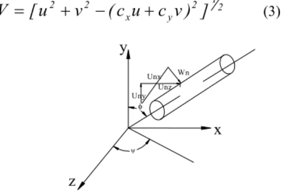
res. Now, the shakedown analysis of the offshore structure under specific combination of nodal loading equivalent to the wave loads is conducted and the shakedown load multiplier is calculated. The multiplier more than unity means the corresponding wave causes the shakedown of the structure.

Shakedown Loading Domain Based upon Airy Linear Wave Theory: Usually, the offshore structures

consist of pipe members in different directions. On the other hand, the wave force applying on an element with variable direction can be easily decomposition into horizontal and vertical components. Consider a pipe element with arbitrary direction in xyz system as shown in Fig. 1. Now, if the movement of the fluid consisting of horizontal component of velocity, v, vertical component of velocity, u, horizontal component of acceleration,

a

_x, and vertical component of acceleration,

a

_y is known, the force resulted from the waves applying on the pipe element can be calculated. In cylindrical system,

φ

and

ψ

indicate the direction of the cylinder. The component of the velocity of the water perpendicular to the cylinder axis, V, can be found using the following relationship [14].

2 1 2 y x 2

2

_v

₍

_c

_u

_c

_v

₎

_]

u

[

V

=

+

−

+

(3)

Wn

ψ Unz

z

Uny

φ y

Unx

x

Fig. 1: A typical tubular element in cylindrical coordinate

The components of the velocity in x, y and z directions are computed from the following relationships.

)

v

c

u

c

(

c

u

u

_n

=

−

_{x x}

+

_y

)

v

c

u

c

(

c

v

v

_n

=

−

_{y x}

+

_y (4)

)

v

c

u

c

(

c

w

_n

=

−

_{z x}

+

_y

where

θ

φ

Cos

Sin

c

_x

=

,

φ

Cos

c

_y

=

,

θ

φ

Sin

Sin

c

_z

=

(5) Also, the components of the wave acceleration in x, y and z directions can be determined as follows,

)

a

c

a

c

(

c

a

a

_nx

=

_x

−

_{x x x}

+

_{y y}

)

a

c

a

c

(

c

a

a

_ny

=

_y

−

_{y x x}

+

_{y y} (6)

)

a

c

a

c

(

c

The components of the force applying per unit length of the cylinder in x, y and z directions are calculated as follows, nx 2 1 n D x a 4 D C DVu C 2 1

f = ρ +ρ π

ny 2 1 n D y a 4 D C Dv C 2 1

f = ρ +ρ π (7) nz 2 1 n D z a 4 D C Dw C 2 1

f = ρ +ρ π

in which

ρ

is the density of the water, D is the diameter of the pipe element of the structure and

I

D

C

C

and

are the drag coefficient and the inertia coefficient of the water particles, respectively. The force perpendicular to the unit length of the pipe element is 2 1 2 z 2 y 2

x f f )

f (

f =± + + (8)

The sign of the force is chosen concerning the signs of

z y

x

f

f

f

,

and

components. So, typically an offshore structure element is under a non-uniform distributed loading along the length of the member based upon (8).

Finite Element Formulation for Shakedown Analysis: Consider a prismatic pipe element to be used for analyzing the offshore structure as shown in Fig. 2. In the modeling, the near and far ends of the element are indicated by i and j, respectively. In the member coordinate system,

{ }

x

,

y

, the x axis is the axis of the member, and the components of the displacement is stated by the movement perpendicular to the cross section of the member in xy plane, such that u(x) is the axial displacement, w(x) is the transverse displacement and

θ

( )

x

is the rotation component. Also, the stresses are corresponding to the axial force, N(x), shear force, V(x), and bending moment, M(x), applying at the cross sections of the member.

θi ui

i

φ_s j φa φs φe φe θj W j uj

Fig. 2: Kinematics parameters and natural modes for element of structure

The axial and shear components are constant but the moment varies linearly. Therefore, the components can be shown as follows [3],

)) 2 1 ( m m ( 2 1 ] x [ M , l m ] x [ V , l m ] x [

N s e

e

a _{=− = + −} ξ

= (9)

So, j i e j i s

a Nl, m M M , m M M

m = = + = − (10)

where

l

=

x

_j

−

x

_i is the member length and

(

x

−

x

_i

)

l

=

ξ

is a dimensionless coordinate which varies in the interval [0,1]. The strain energy of the member can be calculated as follows,

ξ Π d EI M GkA V EA N 2 l 1 0 2 2 2

b

∫



     + +

= (11)

in which A, k and I are the cross sectional area, the shear multiplier of the section and the moment of inertia of the section, respectively. E and G are elasticity and shear modulus, respectively. Moreover, the strain energy can be obtained using Clapeyron theorem as follows,

) M M ) w w ( V ) u u ( N ( 2 1 i j j i i j i j

b θ θ

Π = − + − + − (12)

On the other hand, the natural strains can be defined as follows, l w w l l u

u_{j i s j i e j i j i}

a=( − )/ , φ =(θ −θ)/ , φ =(θ −θ)/2−( − )/

φ

(13)

So, using (9) through (13) the strain energy can be found as follows,

                              = e s a e s a T e s a b k 0 0 0 k 0 0 0 k 2 1 φ φ φ φ φ φ

Π (14)

where 2 e s a GkAl EI 12 , ) 1 ( l EI 12 k , l EI 4 k , EAl k = + = = = β β (15) Based upon Fig. 2, the components of the displacement field for the two ends of the member are,

{

}

T

j j j i i i

b u w u w

u = θ θ (16)

Using the transform matrix of the X and Y coordinate, the relationship between the natural strains and the components of the displacement field can be indicated in the form of the following formula [6].

α α φ φ φ Cos C Sin S 2 / 1 l C l S 2 / 1 l C l S 2 / 1 0 0 2 / 1 0 0 0 l S l C 0 l S l C T , u Tbb b e s a = =           − − − − − = =         

 (17)

b T b b b T b

b

u

K

u

u

F

2

1

_≡

=

Π

(18)

The elastic stiffness matrix and the vector of the internal forces are determined as follows,

          =           = e s a T b b T b e s a T b b m m m T F , T k 0 0 0 k 0 0 0 k T K (19)

So, the total elastic stiffness matrix,

K

_s, and the internal forces vector,

F

_s, in global coordinate system for an offshore structure is found by assembling the values concerning each element as follows,

∑

∑

= = b b b s b

s K , F F

K (20)

Admissible Shakedown Domain: Defining an

admissible domain for yield condition and for forming the plastic hinge in the member is one of the main points in shakedown analysis. For simplicity of the analysis, the bending moment, M, is considered for plastic state only. So, the problem is defined as follows,

) x ( M M ) x (

M_y= ≤ ≤ _y+ (21)

in which

x

∈

[ ]

0

...

l

and

M

_y+

( )

x

and

M

_y−

( )

x

are the positive and negative yield moments, respectively. The response of the basic external elastic moments is as follows, max i i min i P 1 i E i i E ), x ( M ) x (

M =

∑

α α ≤α ≤α

=

(22) Therefore, the maximum and minimum of the responses of the elastic moments are as follows,

)) x ( M max( ) x ( M )), x ( M min( ) x ( M E E E

E = =

+ −

(23)

Now, using the values as determined in the above, the admissible shakedown analysis domain for a member of an offshore structure with i and j ends can be easily defined by the following relationships

+ + − −

₋

_≤

_≤

₋

Ei yi i Ei

yi

M

M

M

M

M

λ

λ

(24)

+ + − −

₋

_≤

_≤

₋

Ej yj j Ej

yj

M

M

M

M

M

λ

λ

(25)

The following relationship can be found using (10),

2

/

)

m

m

(

M

_i

=

_s

+

_e ,

2

/

)

m

m

(

M

_j

=

_s

−

_e (26)

Finally, the largest admissible load multiplier is as follows,         − − = _{+ −} − + Em Em ym ym S M M M M min

λ (27)

Where

m

relates to the control at the end section of all elements of the offshore structure.

Calculation of Shakedown Multiplier under Nodal Equivalent Wave Forces: A collapse mechanism for the plastic rotation,

θ

_m, at the section

m

is defined first. The plastic hinge will be formed under one of the following conditions.     < − = − > = + − + 0 if M M m 0 if M M m m pm min m m m pm max m m θ θ (28)

where

M

_pm+ and

M

−_pmare the maximum and minimum values of plastic moment, respectively, and parameter

m

_m is the residual moment at the sections

{

m

=

1

,

2

,

3

,...

}

and are under equilibrium condition. Therefore, the following relationship can be obtained based upon the virtual work [11].

∑

=

=

⋅

1 m m m

0

m

θ

(29)

Substituting (28) into (29) the following general equation is obtained.

∑

= − + = ⋅         + − − 1 m m min m pm max m pm 0 M M M M

θ (30)

Using transform variable

θ

_m

=

θ

_m+

−

θ

_m− the following relationship is determined.

∑

∑

= = − − + + − +_{+ ⋅ = ⋅ + ⋅} ⋅ 1

m m1

m pm m pm m min m m max

m M ) (M M )

M

( θ θ θ θ (31)

and the parameters of maximum and minimum elastic moment can be indicated as follows,







⋅

=

⋅

=

⋅

=

⋅

=

− +

))

x

(

M

min(

)

x

(

M

M

))

x

(

M

max(

)

x

(

M

M

E a E a min m E a E a max m

λ

λ

λ

λ

(32)

Substituting (32) into (31) the following equation is obtained.

∑

∑

= = − − + + − − + + _{⋅ + ⋅ = ⋅ + ⋅} ⋅ 1

m m1

m pm k pm m E m E

a (M (x) θ M (x) θ ) (M θ M θ )

λ

m )

) x ( M ) x ( M (

) M M

( min

1 m

m E m E 1 m

m pm m pm

a ∀

    

    

⋅ + ⋅

⋅ + ⋅ =

∑

∑

=

− − + + =

− − + +

θ θ

θ θ

λ

(34)

Now, considering the equivalent nodal loads due to the waves obtained in section 2.2 of this paper and applying Quadratic Programming optimization algorithm the relationship (34) is controlled for all the members of the structure and finally the multiplier of the shakedown load,

λ

_S, is computed. It must be noted if the multiplier of the shakedown load is more than unity the multiplier obtained will be the same as a collapse load multiplier.

Domain of the Shakedown Unsafe Waves: For any offshore structure it is necessary to find a repeating wave loads domain under which shakedown of the structure certainly happens. Here, after shakedown analysis of the structure, if the multiplier of the shakedown load is more than unity, the corresponding load combination will be consider as critical shakedown load. In this study, the domain of the waves which cause shakedown is called "unsafe waves domain" for offshore structure shakedown. Now, having different water depth to wave length ratios,

h

L

, and different wave height to wave length ratios,

H

L

, for the critical shakedown load waves, the graph of the domain of the shakedown unsafe waves can be drawn.

Numerical Studies

Example 1: An offshore platform Frame with X Bracings: Fig. 3 shows the characteristics of the offshore platform structure. The structure has been divided into 14 elements. The crest of the wave amplitude is taken such that the maximum shear force and bending moment is developed in the structure. Then, the forces caused by a wave with specific characteristics are determined using Airy wave theory and converted into equivalent nodal loads.

6 8 3 5 1 2

4

7

y x

l

l

l

Fig. 3: Offshore platform frame considered in numerical example 1

l=6943 Cm

D=120 Cm Column Diameter D1=60 Cm Beam & Bracing Diameter t=2.5 Cm thickness of D

t1=1.25 Cm thickness of D1

2

2400 Kg_Cm y

F =

2

6 10 03 .

2 Kg_Cm

E= ×

Afterwards, the shakedown analysis has been done using static Melan theorem and an optimization algorithm and the shakedown multiplier has been found for the specific wave. If the shakedown multiplier is more than or equal to unity, the wave is critical and its characteristics will be recorded. This process is repeated for all the waves that are possibly encountered the structure. At the end, the critical region in which the shakedown happens is assigned on a graph. The details of the information obtained for example 1 is shown in Fig. 4. As it can be seen, the graph has been drawn for all the values of ratios

h

L

and

H

L

obtained from Airy theory. The hashed region shows the waves that if apply on the structure repeatedly, the collapse mechanism forms and the structure shakedown happens. So, a part of the region is critical. For other values, the region is called "safe for shakedown".

Fig. 4: Critical region for shakedown in example 1

wave load

l

l

ll

1 4 2

3 7 5

6 8

Fig. 5: Offshore structure considered in numerical example 2

l=7000 Cm

D=30 Cm Column Diameter D1=20 Cm Beam & Bracing Diameter t=1.5 Cm thickness of D

t1=1.0 Cm thickness of D1

2

2400 Kg_Cm y

F =

2

6 10 03 .

2 Kg_Cm

E= ×

-60 -40 -20 0 20 40 60

-50 -30 -10 10 30 50

1e3 (rad) M(ton-m)

(a) beam and bracing member

-15 -10 -5 0 5 10 15

-40 -20 0 20 40

1e3 (rad) M(ton-m)

(b) column

Fig. 6: Material behavior models for structure considered in numerical example 2

The finite element model of the structure including members and nodes has been prepared first, and then the wave loading defined by Airy theory has been

applied on the structure. In the next step, the shakedown multiplier for the equivalent nodal load due to the maximum wave amplitude has been calculated using shakedown analysis. Then, the unsafe region for critical shakedown load multiplier has been drawn as shown in Fig. 7. As mentioned before, the dashed region indicates the waves characteristics that cause the structure shakedown when they arise.

Fig. 7: Critical region for shakedown in example

CONCLUSION

In this paper a simple and practical formulation for shakedown analysis of offshore structures under wave loads has been developed. The static Melan theorem for shakedown analysis of the structures having elastic-plastic behavior have been stated first. Then a simple finite element model with pipe type elements have been used for analyzing the structure frames of the offshore structure. In the next step, the loads due to the sea waves that may arise during the structure life have been evaluated using Airy wave theory. The maximum forces that may be applied on the structure members regarding the velocity and acceleration of the pick waves using Morison relationships. The equivalent nodal loads due to the maximum of the sea waves have been used for shakedown analysis of the structure in order to find the shakedown load multiplier. Finally, the waves that cause forming the collapse mechanism in the members and so, the structure shakedown, when they arise and are repeated, have been distinguished from the other waves by a graph.

previously must be evaluated for shakedown and if the unsafe waves concerning shakedown may happen at the site that those structures are located, they must be strengthen in this regard. The method developed in this paper is suitable for large offshore structures because of its simplicity. Also, the proposed method can help the designers for designing the geometry of the structure and choosing the materials characteristics.

REFERENCES

1. Borino G., Polizzotto C., 1995. Dynamic shakedown of structures under repeated seismic loads. Journal of Engineering Mechanics. 1306– 1314.

2. Capurso M., 1974. A displacement bounding principle in shakedown of structures subjected to cyclic loads, International Journal of Solids & Structures. 10: 77–92.

3. Casciaro R., Garcea G., 2002. An iterative method for shakedown analysis, Computer Methods in Applied Mechanics and Engineering. 191: 5761-5792.

4. Corradi L. and Zavelani A., 1974. A linear programming approach to shakedown analysis of structures. Computer Methods in Applied Mechanics and Engineering. 3: 37–53.

5. Dawson T. H., 1983. Offshore structural engineering. 1 st. ed. , Prentice Hall, Englewood Cliffs, N.J., USA

6. Garcea G., Armentano G., petrolo S. and Casciaro R., 2005. Finite element shakedown analysis of two-dimensional structures, International Journal of Numerical Methods in Engineering. 1174-1202 7. Janas M., Pycko S. and Zwolinski J., 1995. A min–

max procedure for the shakedown analysis of skeletal structures. International Journal of Mechanics Science. 37 (6): 629–643

8. Koiter W.T., 1956. A new general theorem on shakedown of elastic–plastic structures. Proc. Koninkl. Ned. Akad. Wet. B 59, 24-34

9. Konig A., Maier G., 1981. Shakedown analysis of elasto plastic structures: a review of recent developments. Nuclear Engineering Design. 66: 81-95

10. Konig A., 1987. Shakedown of elastic–plastic structures, Fundamental Studies in Engineering 7, Elsevier

11. Maier G., Shakedown analysis, in: Cohn M. Z., Maier G., 1979. Engineering Plasticity by Mathematical Programming, Pergamon Press. 107– 134

12. Maier G., Carvelli V. and Cocchetti G., 2000. On direct methods for shakedown and limit analysis, Plenary Lecture, 4th Euromech Solid Mechanics Conference, Metz, June 2000, European Journal of Mechanics and Solids. 19 (special issue): S79– S100

13. Melan E., 1938. Zur Plastizitat des raumlichen continuum, Ing. Arch. 9: 116–126

14. Noorzaei J., Bahrom S. and Saleh jaafar M., 2005. Simulation of wave and current forces on template offshore platforms, Suranaree Journal of Science & technology. 12(3): 193-210

15. Pham D.C., 2001. Shakedown kinematic theorem for elastic-perfectly plastic bodies. International Journal of Plasticity. 17: 773-780

16. Ponter A.R.S. and Karter K.F., 1997. Shakedown state simulation techniques based on linear elastic solutions, Computer Methods in Applied Mechanics and Engineering. 140: 259–279

17. Ponter A.R.S., Engelhradt M., 2000. Shakedown limits for a general yield condition: implementation and application for a von Mises yield condition. European Journal of Mechanics and Solids. 19: 423–445

18. Polizzotto C., 1993. On elastic plastic structures under cyclic loads. European Journal of Mechanics and Solids. 149–173