Edgard Poiate Jr.
[email protected] PETROBRAS - Brazilian Petroleum S.A Scientific Methods Group at R&D Center 21941-598 Rio de Janeiro, RJ. BrazilJosé Luiz Gasche
Senior Member, ABCM [email protected] State University of São Paulo - UNESP Department of Mechanical Engineering 15385-000 Ilha Solteira, SP. BrazilFoam Flow of Oil-Refrigerant R12
Mixture in a Small Diameter Tube
This paper presents an experimental investigation of the mineral oil ISO VG10-refrigerant R12 mixture flow with foam formation in a straight horizontal 3.22 mm ID, 6.0 m long tube. An experimental apparatus was designed to allow the measurement of both pressure and temperature profiles along the tube as well as the visualization of the flow patterns. Tests were performed at different mass flow rates, several refrigerant mass fractions at the inlet of the flow, and inlet mixture temperatures around 29.0 °C. At the inlet of the tube a liquid mixture flow was visualized. In this region, both temperature and pressure gradient were constant. As the flow proceeded towards the exit of the tube the pressure drop produced a reduction of the refrigerant solubility in the oil yielding to the formation of the first bubbles. Initially, small and few bubbles could be noticed and the flow behaved as a bubbly flow. Eventually, the bubble population increased and foam flow pattern was observed at the exit of the tube. Due to the large formation of bubbles, both the temperature and the pressure of the mixture were substantially reduced in this region. Visualization results also showed that both flow regimes (bubbly and foam) were intermittent.
Keywords: Oil-refrigerant mixture, foam flow, two-phase flow pattern, flashing flow
Introduction
Regarding the refrigeration cycle a good miscibility of the refrigerant in the lubricating oil is required in order to allow easy return of circulating oil to the compressor through the reduction of the oil viscosity. However, inside the compressor this miscibility considerably modifies the leakage of the refrigerant gas through the clearances, the lubrication of sliding parts, and the performance of journal bearings. The solubility of the refrigerant in the lubricating oil depends on the oil temperature and refrigerant vapor pressure, diminishing as the temperature increases or the pressure decreases. Consequently, as the mixture flows through the several types of channels inside the compressor, the refrigerant evaporates from the oil-refrigerant mixture (outgassing) due to the reduction of the solubility caused by the friction pressure drop.
As an example of this type of problem one can use the work of Costa et al. (1990), who performed a visualization experiment to study the refrigerant gas leakage through the radial clearance in a rolling piston compressor running in regular operational condition. They showed the existence of bubbles just after the minimal clearance and observed that the number of bubbles was so large that they seemed to form a foam. Kraynik (1988) defines foam as a structured fluid in which gas bubbles are separated by thin liquid films and the volume fraction of the continuous liquid phase is small. Winkler et al. (1994) commented that void fraction value typically of about 0.7 is very common for foams. What is important about this issue is that foam flow behaves in a different way from the conventional (bubbly, slug, annular, etc.) two-phase flows, Calvert (1990), mainly because it flows as a non-newtonian fluid.
Therefore, from the point of view of the compressor, a general understanding of the oil-refrigerant mixture flow with foam formation through small channels is crucial in order to develop a knowledge basis onto which lubrication and gas leakage models can be built.1
Mainly in the 80’s and 90’s, several studies related to oil-refrigerant mixture started being developed. Some of these works were directed towards the determination of the thermophysical properties of the new mixtures (Martz et al.; 1996, Grebner and Crawford., 1993; Thomas and Pham, 1992; Baustian et al., 1986; Thome, 1995; and Van Gaalen et al., 1990, 1991a, 1991b). Other
Paper accepted June, 2006. Technical Editor: Aristeu da Silveira Neto.
researchers concentrated their studies on the behavior of refrigerant flows contaminated with lubricating oil (refrigerant-rich mixtures) with the objective of analyzing the influence of the oil in the mixture flow and heat transfer dynamics in evaporators and condensers. In these studies the emphasis was placed in oil-refrigerant mixtures with low oil concentration. Some examples of these researchers are Schlager et al. (1987), Jensen and Jackman (1984), and Wallner and Dick (1975), Hambraeus (1995).
Motta et al. (2001) provided a good literature review on oil-refrigerant mixture flows. It is very interesting to note from their analysis that most of the studies are related to mixture flows with a low oil mass fraction (less than 5%), that is, the oil is treated as the contaminant. There have been very few studies of oil-refrigerant flow in which the oil is contaminated by the refrigerant, which is an important issue when one intends to analyze the compressor behavior.
One of these works was accomplished by Lacerda et al. (2000), who presented an experimental research on oil-refrigerant two-phase flow through a long tube using mineral oil and R12 as refrigerant. They measured the pressure and temperature profiles of the flow through a 2.86 mm-diameter Bundy type tube. Furthermore, they visualized the flow patterns of the same mixture flowing through a 3.03 mm-diameter glass tube. The visualization results showed a foam flow at the end of the tube, where they observed a large reduction in both temperature and pressure.
Recently, Barbosa Jr. et al. (2004) presented an analysis of the available prediction methodologies for frictional pressure drop in two-phase gas-liquid flows of oil-rich refrigerant-lubricant oil mixtures in a small diameter tube. Several correlations and methods for the calculation of the frictional two-phase pressure drop were investigated by the authors, some of them being state-of-art methods developed based on data for small diameter channels. They found none of the methodologies perform satisfactorily over the range of conditions covered during R12-mineral oil mixture flow tests in a 5.3 m long 2.86 mm diameter tube. Then, they proposed a new correlation to predict the frictional pressure drop for this mixture.
ID tube will be presented. In addition, the flow patterns will also be presented.
Nomenclature
ID = inner diameter of the tube, m f = friction factor, dimensionless p = pressure, bar
Re = Reynolds number, dimensionless V = average velocity, m/s
w = refrigerant mass fraction, kg of refrigerant/kg of mixture x = quality, dimensionless
z = longitudinal coordinate, m Greek Symbols
α = void fraction, dimensionless = dynamic viscosity, kg/(m s)
ρ
= density, kg/m3
Subscripts i = inlet in = initial t = test g = vapor phase l = liquid mixture
Experimental Method
The experimental apparatus was designed to produce steady flows of an oil-refrigerant mixture through two 6 m long tubes in such a way that three types of flow patterns could be observed along the flow: a liquid mixture flow at the entrance of the tube, an intermediary two-phase region, and a foam flow in a region near the end of the tube. A metallic tube was instrumented with pressure transducers and thermocouples in order to measure the pressure and temperature distribution along the flow. A glass tube was used to allow for the visualization of the flow patterns.
Apparatus and Instrumentation
A scheme of the experimental apparatus is depicted in Fig. 1. The main components of the test facility are the four tanks, the test section (two horizontal tubes), a vapor return line, an oil return line, instrumentation, and a data acquisition system. All these equipments are connected with each other in order to produce the flow through either of two 6 m long horizontal tubes. The first tube is made of borosilicate glass (3.0 mm ID) and allows flow visualization. The other tube is a metallic 3.22 (±0.03) mm ID tube equipped with 10 absolute pressure transducers based in strain-gauge sensor -type P8AP made by HBMTM- and 14 AWG 36 type-T thermocouples. The pressure transducers were calibrated using a dead weight calibrating machine, resulting in a 2-σ uncertainty of ±2 kPa, and were installed along the tube through 0.3 mm pressure taps. The type-T thermocouples were calibrated using a 0.1°C-resolution mercury-in-glass thermometer and the 0°C-electronic reference of the data acquisition system, resulting in a 2-σ uncertainty of ±0.5°C. They were installed through a superficial role made on the tube surface. Thermocouple and pressure readings were hardwired into a HBMTM data acquisition system (Spider8 and MGCplus) and routed directly to a personal computer. Data interpretation and manipulation was performed using the software package CatmanTM by HBMTM. Specific details regarding the experimental apparatus,
instrumentation, calibration procedure, and data acquisition system can be obtained from the study of Poiate Jr. (2001).
The main objective of the four tanks is to maintain constant the pressure difference between the high and the low-pressure tanks
(HPT, LPT), which are connected by the two tubes. The HPT is filled with oil and refrigerant, and an equilibrium liquid mixture at the bottom of the tank coexists with the refrigerant vapor at the top for the desired temperature and vapor pressure. Pressure and temperature sensors monitor the conditions of the gas and liquid in both tanks. High and low pressure accumulators (HPA, LPA) operating at pressures higher and lower than those at HPT and LPT, respectively, keep the pressure at constant levels in both tanks using two automatic solenoid valves controlled by a desktop computer. During operation the equilibrium liquid mixture existing in HPT is driven into either of the two tubes. The experimental apparatus runs on the blow down mode.
Auxiliary equipment consist of a compressor, an oil pump, and two heat exchangers (HE1, HE2). The compressor is employed to return the gas to the HPA and the pump returns the oil back to the HPT for undertaking other tests. The heat exchangers are used to cool both fluids if necessary before reaching the HPA and HPT.
Experimental Procedure
Firstly, the necessary parts of the apparatus were cleaned with a solvent fluid to remove impurities, and the system was evacuated to 10 Pa. After that, 80 kg of mineral oil ISO VG10 were introduced into the HPT and heated until 60ºC for three hours in order to remove impurities (mainly water), while the vacuum pump was kept running. Next, 60 kg of R-12 were introduced partly into the HPT and HPA.
All tests started with the saturation of the oil in the HPT at the desired test temperature and 100 mbar above the desired test pressure, pt, that is, at an initial pressure, pin=pt+0.100 bar. In order
to increase the rate of absorption, the refrigerant was bubbled in the HPT by employing the compressor, which sucked the refrigerant gas from the top and compressed it at the bottom of the HPT. As the liquid mixture absorbed gas, the pressure tended to decrease, activating the automatic solenoid valve (SV1), which released refrigerant from HPA to HPT in order to maintain the pressure in the HPT constant. This process continued until saturation was achieved in the HPT at pin. The saturation process could last until six
hours. After saturation was reached at pin some amount of gas was
released from the top of HPT to decrease the pressure to pt, the
desired test pressure. This pressure reduction promoted a fast outgassing and assured that saturation was indeed established at pressure pt (±1% of the value). This new saturation state was
reached within 30 to 60 minutes, which was observed when pressure stopped increasing because of the gas release. The temperature was controlled at the desired value (±1°C) during all this process.
Depending on whether flow visualization or measurement run was desired, after the saturation process is finished, the test section valves were arranged so that the mixture was forced into the glass or the metallic tube, respectively. During the experimental runs the compressor remained running in order to circulate gas from the LPA to the HPA. Data acquisition was initiated after the steady flow was reached. The steady state regime was characterized by observing the time variation of the mixture temperature in all measuring position. When the variation temperature was of the order of 0.5°C it was assumed that the steady state flow was reached.
the validation of the experimental apparatus can be found in Poiate Jr. (2001).
HPT
HPA LPA
pump
compressor
HE1
HE2
SV1 SV2
glass tube metallic tube
LPT refrigerant
vapor
mixture
Figure 1. Experimental apparatus.
Data Reduction and Interpretation
A mass flow meter could be installed just after the HPT to measure the mass flow rate of the flow. However, this device would cause a pressure drop in the flow so that an undesired outgassing could happen before the liquid mixture flow reached the tube (the test facility was conceived so that the outgassing started inside the tubes). In order to avoid this problem the mass flow rate was not measured. Instead, the mass flow rate was calculated by using the pressure gradient measured at the inlet region of the flow, where the mixture was still in the liquid state and the flow could be considered as completely developed, because the pressure gradient measured in that region was constant. The average velocity used to determine the mass flow rate was calculated using Equation (1):
2 / 1
l dz
dp f D 2
V
− ρ
= (1)
where D is the tube diameter, ρl is the density calculated at the inlet
temperature of the mixture, f is the friction factor calculated by the equation proposed by Churchill (1977), and (dp/dz) is the pressure gradient along the flow direction measured at the linear region of the pressure distribution.
The Reynolds number is defined as,
l lVD
Re µ ρ
= (2)
where µl is the absolute viscosity of the liquid mixture at the inlet of
the tube. Both properties, µl and the saturation mass fraction of the
refrigerant in the oil, w, were taken from the oil manufacturer. It would be interesting to have an idea about the order of magnitude of the void fraction along the flow. In order to do that a very simple model was developed to calculate this variable using the experimental data of the pressure and temperature profiles as primary variables. First of all, it was assumed that the liquid mixture remained always saturated along the flow, that is, it was considered that the local thermodynamics equilibrium existed. This assumption seemed to be reasonable since the outgassing usually occurs almost instantaneously.
Using this hypothesis one can determine the local quality at any position z along the flow, x, by applying the mass conservation principle to the mixture flow, which results in the following equation:
w 1
w w
x e
− −
= (3)
where w is the local mass fraction at the position z, calculated at the local experimental pressure and temperature condition, and we is the
mass fraction at the beginning of the bubble nucleation, which was assumed to happen when the temperature started to decrease, therefore, determined at this temperature and pressure.
The local void fraction can be easily estimated by Equation (4), assuming that the homogeneous two-phase flow model is adequate to represent the flow. The homogeneous model considers the two-phase flow as a single-two-phase flow possessing mean fluid properties. The basic premises upon the model is based are the assumptions of equal vapor and liquid velocities, and thermodynamic equilibrium between the phases. The homogeneous model was chosen here because, besides being the simplest model, the predominant flow patterns visualized in this work were the bubbly and foam flow, which are more adequate to this type of model. The void fraction is, therefore,
1 x l
) x 1 ( g
1
− ρ
− ρ
+
=
α (4)
where ρg is the refrigerant density in the vapor state at the local
pressure and temperature (to this condition, the thermodynamic state of the gas is superheated vapor for the local pressure and temperature), and ρl is the liquid mixture density at the same
condition. The liquid mixture was assumed to be an ideal solution with a correction factor suggested by ASHRAE (1998).
The local density of the two-phase flow can be estimated using the following equation:
l g+(1−α)ρ
ρ α =
ρ (5)
Reduced Data Uncertainty
The uncertainties of the reduced data were determined by propagating the measurement uncertainties using standard methods (Moffat, 1988). The uncertainty of the average velocity was ±5%, while the uncertainty of the Reynolds numbers was ±10%. The uncertainty of the average velocity depends on the pressure gradient at the inlet of the flow and was estimated by the uncertainty of the pressure curve fitting accomplished in that region, taking in account the uncertainties of the temperature (± 0.5°C) and pressure (±2 kPa).
Results
More than thirty tests were undertaken using a mixture composed by a mineral oil ISO VG10 and refrigerant R12. Pressure and temperature profiles were measured, and visualization results were accomplished for all tests. The results for 18 tests are presented in order to show the main characteristics of the flow. The test 18 was chosen as a representative visualization result among all them. The operational conditions of the tests are depicted in Table 1. The HPT pressures were chosen in such a way that foam flow could be observed at the exit region of the tube.
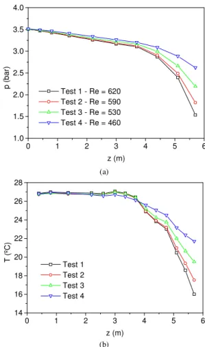
Pressure and temperature distribution for tests 1 to 4 are shown in Figs. 2(a) and 2(b), respectively. Pressure and temperature results are average values from measurements taken during about 3 minutes after steady state was established.
presence of few small bubbles in this region, which could be visualized in a similar flow through the glass tube, was not sufficient to change the single-phase flow characteristics. The constant temperature measured in this region, which is shown in Fig. 2(b), confirms the single-phase flow characteristics. Downstream the position z=3.5 m, the pressure gradient starts to increase also due to the outgassing from the liquid mixture, which causes density reduction at each cross section along the flow. Consequently, the flow accelerates and the pressure drop considerably increases to comply with both friction and fluid acceleration. As pressure decreases and gas is released from the liquid mixture, the temperature decreases to keep up with the latent heat requirements for evaporation. Figs. 2(a) and 2(b) show that the pressure and temperature profiles are qualitatively similar. However, as could be expected, the total pressure drop increases with the Reynolds number. Fig. 2(b) shows that the larger the total pressure drop the larger the total temperature reduction due to the increasing outgassing. One can observe that the total temperature reduction varies from about 5 for Re=460 to 11 ºC for Re=620. One can notice that the Reynolds number in all these tests was kept in the range of laminar flow.
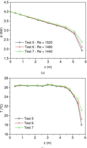
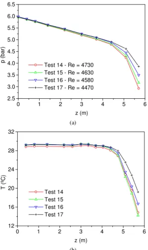
Figure 3 presents pressure and temperature profiles for the tests 5 to 7, which were accomplished for higher Reynolds numbers and inlet mass fractions. One can observe that the results are qualitatively similar and the same discussion of the Fig. 2 can apply for these tests. However, for these new conditions, one can notice that the two-phase flow starts at about z=4 m, which is the position in which the temperature starts to decrease. The total temperature reduction in these tests varies from about 5 to 8 ºC, and the Reynolds number of the tests still was kept in the range of laminar flow. Similar behavior for the pressure and temperature profiles can be observed for the tests 8 to 10 in Fig. 4, tests 11 to 13 in Fig. 5, and tests 14 to 18 in Fig. 6.
The more important conclusion from all these results is that there are two different flow regions: at the inlet of the tube, up to about 3.5 to 5 m, the pressure gradient and the temperature are constant, which indicates that the single phase flow prevails regardless of the presence of few small bubbles (these bubbles were visualized in similar flows through the glass tube); the other region at the end of the tube is characterized by large pressure and temperature reduction, suggesting that the outgassing increased substantially (this conclusion was made with the help of the visualization results through the glass tube).
Table 1. Operational conditions of all tests.
Test HPT Pressure
(bar)
LPT Pressure
(bar)
Inlet Temperature
(oC)
Inlet R12 Mass Fraction,
wi
Reynolds Number,
Re
01 1.00 26.8 0.25 620
02 1.50 26.7 0.25 590
03 2.00 26.7 0.25 530
04 3.50
2.50 26.7 0.25 460
05 1.00 26.3 0.31 1520
06 1.50 26.5 0.31 1480
07 4.00
2.00 26.5 0.31 1440
08 2.00 26.3 0.39 1930
09 2.50 26.3 0.39 1880
10 4.50
3.00 26.3 0.39 1800
11 1.00 29.7 0.41 3380
12 1.50 30.1 0.41 3030
13 5.00
2.00 29.1 0.43 3060
14 2.00 28.9 0.64 4730
15 2.50 29.2 0.63 4630
16 3.00 29.2 0.64 4580
17 6.00
3.50 29.2 0.63 4470
18 5.50 1.50 31.5 0.46 4310
0 1 2 3 4 5 6
1.0 1.5 2.0 2.5 3.0 3.5 4.0
Test 1 - Re = 620 Test 2 - Re = 590 Test 3 - Re = 530 Test 4 - Re = 460
p
(
b
a
r)
z (m)
(a)
0 1 2 3 4 5 6
14 16 18 20 22 24 26 28
Test 1 Test 2 Test 3 Test 4
T
(
ºC
)
z (m)
(b)
Figure 2. Pressure and temperature distribution for tests 1 to 4.
In order to produce at least the magnitude of other important variables of two-phase flows, Eqs. (3) to (5) were used to estimate the quality, void fraction, and flow density profiles for test 14 as a representative example. Figure 7 shows the experimental pressure and temperature profiles, plotted by the black squares. Analyzing the temperature data it was assumed that the bubble formation started at z=3.7 m, which was the last position before occurring the first significant temperature drop, called here by ze. For z≤ze it was
assumed that the temperature remained constant, given by the average value of the experimental data. These data are represented by black squares and named fitted data in Fig. 7(b). This figure also shows a point represented by a hollow triangle, which was removed from the data because it produced a physically inconsistent behavior for the other variables (w, x, α, and ρ).
As it would be expected the quality and the void fraction start increasing after the beginning of the bubble formation. Otherwise, the flow density starts decreasing from this point forward. From Fig. 9(a) one can observe that the void fraction reaches high values. Void fractions of this order of magnitude would probably indicate annular flow pattern for conventional two-phase flows. The visualization results, however, depict foam formation for high void fraction values. It is important to emphasize that this type of flow pattern is not found in conventional two-phase flows.
that foam flow is generally observed when the void fraction reaches values typically of about 0.7. This is an important conclusion one can draw from these results: from the experimental temperature and pressure profiles together with the visualization results it was possible to prove the existence of the foam flow pattern for the mineral oil-refrigerant R12 mixture flow through a straight circular tube when the void fraction reaches high values, around 0.8 for these tests. This kind of flow pattern is not observed for conventional two-phase flows.
0 1 2 3 4 5 6
1.5 2.0 2.5 3.0 3.5 4.0 4.5
Test 5 - Re = 1520 Test 6 - Re = 1480 Test 7 - Re = 1440
p
(
b
a
r)
z (m)
(a)
0 1 2 3 4 5 6
16 18 20 22 24 26 28
Test 5 Test 6 Test 7
T
(
ºC
)
z (m)
(b)
Figure 3. Pressure and temperature distribution for tests 5 to 7.
0 1 2 3 4 5 6
2.0 2.5 3.0 3.5 4.0 4.5 5.0
Test 8 - Re = 1930 Test 9 - Re = 1880 Test 10 - Re = 1800
p
(
b
a
r)
z (m)
(a)
Figure 4. Pressure and temperature distribution for tests 8 to 10.
0 1 2 3 4 5 6
12 14 16 18 20 22 24 26 28
Test 8 Test 9 Test 10
T
(
ºC
)
z (m)
(b)
Figure 4. (Continued).
0 1 2 3 4 5 6
2.0 2.5 3.0 3.5 4.0 4.5 5.0 5.5
Test 11 - Re = 3380 Test 12 - Re = 3030 Test 13 - Re = 3060
p
(
b
a
r)
z (m)
(a)
0 1 2 3 4 5 6
2.0 2.5 3.0 3.5 4.0 4.5 5.0 5.5
Test 11 - Re = 3380 Test 12 - Re = 3030 Test 13 - Re = 3060
p
(
b
a
r)
z (m)
(b)
0 1 2 3 4 5 6
2.5 3.0 3.5 4.0 4.5 5.0 5.5 6.0 6.5
Test 14 - Re = 4730 Test 15 - Re = 4630 Test 16 - Re = 4580 Test 17 - Re = 4470
p
(
b
a
r)
z (m)
(a)
0 1 2 3 4 5 6
12 16 20 24 28 32
Test 14 Test 15 Test 16 Test 17
T
(
ºC
)
z (m)
(b)
Figure 6. Pressure and temperature distribution for tests 14 to 17.
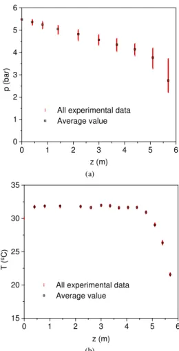
Test 18 was picked to present a typical visualization result. Fig. 10 shows the pressure and temperature profiles for test 18 including all experimental data measured at each position z. Continuous lines are used to represent these data. The average values (plotted by a hollow square) at each position z are also shown in this figure. One can notice in Fig. 10(a) the pressure variation at each position z. This pressure variation is not due to the experimental uncertainty, but an indicative of the intermittence of the flow.
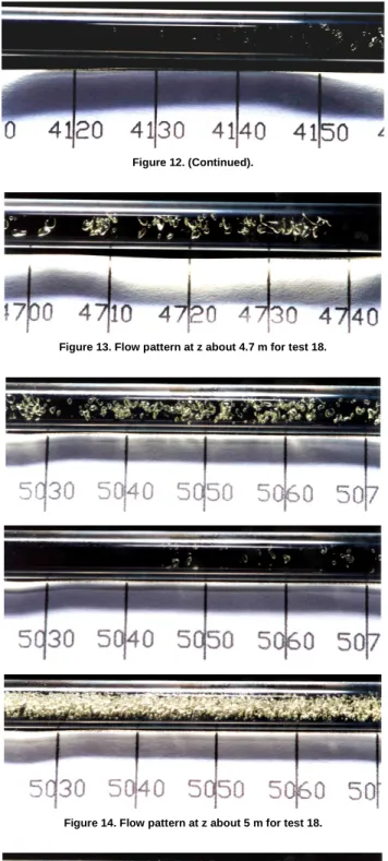
The visualization results depicted in Figs. 11 to 16, which show several photographs taken from the flow at the same position z in different times, can help to prove that the intermittence exists. It is possible to identify different flow patterns at the same position along the flow. In Fig. 11, at z about 3.6 m, one can observe that few small bubbles distributed over the entire cross section of the tube characterize the flow pattern. In Fig. 12, the same type of flow pattern can be noticed, however, with larger bubbles than in Fig. 11. The intermittent flow can be noticed in this test: the first picture shows no bubble, whereas the second depicts some small bubbles. This intermittent flow produces the pressure variation shown in Fig. 10(a). Figure 13 shows that downstream at z=4.7 m the bubbles increase in number as well as in dimension. The intermittent flow still remains at this position.
The number of bubbles continues to increase as z increases, as shown in Figs. 14 to 16. For z larger than 5 m one can notice the existence of the foam flow pattern. At times, no bubble can be visualized at this region (not depicted), showing that the intermittent flow still remains, which also explains the large pressure variation at
the end of the tube. It was possible to notice that at the end of the tube the foam flow was more stable.
From these results one can conclude that there are only two flow patterns for the oil-refrigerant mixture flow: intermittent bubbly flow and intermittent foam flow. All the results shown in this work are qualitatively similar to those obtained by Lacerda et al. (2000) for the same mixture.
0 1 2 3 4 5 6
2 3 4 5 6 7
p
(
b
a
r)
z (m)
(a)
0 1 2 3 4 5 6
10 15 20 25 30 35
Experimental data Fitted data Removed datum
T
(
O C
)
z (m)
(b)
Figure 7. Experimental pressure and temperature profiles for test 14.
0 1 2 3 4 5 6
0.25 0.30 0.35 0.40 0.45 0.50 0.55 0.60 0.65
z (m)
w
(a)
0 1 2 3 4 5 6 0.00
0.05 0.10 0.15 0.20 0.25
z (m)
x
(b)
Figure 8. (Continued)..
0 1 2 3 4 5 6
0.0 0.2 0.4 0.6 0.8 1.0
z (m)
α
(a)
0 1 2 3 4 5 6
0 200 400 600 800 1000 1200
z (m)
ρ
(
kg
/m
3 )
(b)
Figure 9. Calculated void fraction and density profiles for test 14.
0 1 2 3 4 5 6
0 1 2 3 4 5 6
All experimental data Average value
p
(
b
a
r)
z (m)
(a)
0 1 2 3 4 5 6
15 20 25 30 35
All experimental data Average value
T
(
ºC
)
z (m)
(b)
Figure 10. Pressure and temperature fluctuation for test 18.
Figure 11. Flow pattern at z about 3.6 m for test 18.
Figure 12. (Continued).
Figure 13. Flow pattern at z about 4.7 m for test 18.
Figure 14. Flow pattern at z about 5 m for test 18.
Figure 15. Flow pattern at z about 5.3 m for test 18.
Figure 15. (Continued).
Figure 16. Flow pattern at z about 5.8 m for test 19.
Conclusions
physical models to be used in analysis and simulation of lubricating and leakage processes occurring inside refrigeration compressors.
A liquid mixture flow with constant temperature and pressure gradient could be seen at the inlet of the tube. As the flow proceeded towards the exit of the tube the pressure drop produced a reduction of the refrigerant solubility in the oil, yielding to formation of bubbles. Initially, small and few bubbles could be noticed and the flow pattern could be characterized as bubbly flow. Eventually, the bubble population increased and foam flow pattern was observed at the exit of the flow, at about 5 m downstream of the inlet of the tube, where the void fraction was about 0.8. Due to the high bubble formation, both temperature and pressure of the mixture were largely reduced in this region of the flow. Visualization results also showed that both flow regimes were intermittent.
Acknowlegment
This research was supported by FAPESP - São Paulo State Research Foundation.
References
ASHRAE, 1998, Lubricants in refrigerant systems, in ASHRAE Handbook – Refrigeration, Chapter 7, p. 7.1-7.24.
Barbosa Jr., J.R., Lacerda, V.T., Prata, A.T., 2004, Prediction of pressure drop in refrigerant-lubricant oil flows with high contents of oil and refrigerant outgassing in small diameter tubes, Int. J. Refrig., Vol. 27, p. 129-139.
Baustian, J. J., Pate, M. B. and Bergles, A. E., 1986, Properties of oil-refrigerant mixtures liquid with applications to oil concentration measurements: part I – thermophysical and transport properties, ASRHAE Transactions, Vol. 92, p. 55-73.
Calvert,J.R., 1990, Pressure drop for foam flow through pipes, Int. J. Heat and Fluid Flow, Vol. 11 N° 3, p.236-241.
Churchill, S.W. 1977, Friction-factor equation spans all fluid-flow regimes, Chem. Eng., n.7, p. 91-92.
Costa, C.M.F.N., Ferreira, R.T.S., Prata, A.T., 1990, Considerations about the leakage through the minimal clearance in a rolling piston compressor, International Compressor Conference at Purdue, West Lafayette-IN, Vol. II, p. 853-863.
Grebner, J. J., Crawford, R. R., 1993, Measurement of pressure temperature-concentration relations for mixtures of R12/mineral oil and R134a synthetic oil, ASHRAE Transactions, Vol. 99, Part 1, p. 387-396.
Hambraeus, K. 1995, Heat transfer of oil-contaminated HFC134a in a horizontal evaporator, Int. J. Refrig. Vol. 18, N. 2, p. 87-99.
Jensen, M.K., Jackman, D.L., 1984, Prediction of nucleate pool boiling heat transfer coefficients of refrigerant-oil mixtures, J. Heat Transfer, Vol. 106, p. 184-190.
Kraynik, A.M., 1988, Foam flows, Annual Review of Fluid Mechanics, Vol. 20, p. 325-357.
Lacerda, V.T., Prata, A.T., Fagotti, F., 2000, Experimental Characterization of oil-refrigerant two-phase flow, Prof. ASME-Adv. En. Sys. Div., San Francisco, p. 101-109.
Martz, W.L., Burton, C.M., Jacobi, A.M., 1996, Local composition modelling of the thermodynamic properties of refrigerant and oil mixtures, Int. J. Refrig., Vol. 19, No 1, p. 25-33.
Moffat, R.J., 1988, Describing the uncertainties in experimental results, Exp. Thermal Fluid Sci., Vol. 1, p 3-17.
Motta, S.F.Y., Braga, S.L., Parise, J.A.R., 2001, Experimental study of adiabatic capillary tubes: critical flow of refrigerant/oil mixtures, HVAC & R. Research, No 7, p. 331-344.
Poiate Jr., E., 2001, Two-phase flow of the mineral oil-refrigerant R12 through a straight round tube, MEng. Dissertation (in Portuguese), São Paulo State University, Ilha Solteira-SP, Brazil, 216 p.
Poiate Jr., E., Gasche, J.L., 2002, Pressure and temperature distribution and flow visualization of the two-phase mineral oil-R12 mixture (in Portuguese), Brazilian Cong. of Thermal Eng. Sci., paper code CIT02-0843.
Schlager, L. M., Pate, M. B., Bergles, A. E., 1987, A survey of refrigerant heat transfer and pressure drop emphasizing oil effects and in-tube augmentation, ASHRAE Transactions, Vol. 93, Part 1, p. 392-415.
Thomas, R. H. P., Pham, H. T., 1992, Solubility and miscibility of environmentally safer refrigerant/lubricant mixtures, ASHRAE Transactions, Vol. 98, Part 1, p. 783-788.
Thome, J.R., 1995, Comprehensive thermodynamic approach to modeling refrigerant-lubricant oil mixtures, HVAC & R. Research, Vol. 1, No 2, p. 110-126.
Van Gaalen, N.A., Pate, M.B., Zoz, S.C., 1990, The measurement of solubility and viscosity of oil/refrigerant mixtures at high pressures and temperatures: test facility and initial results for R22/naphthenic oil mixtures, ASHRAE Transactions, Vol. 96(2), p.183-190.
Van Gaalen, N.A., Zoz, S.C., Pate, P.E., 1991a, The solubility and viscosity of solutions of R502 in a naphthenic oil and in an alkylbenzene at high pressures and temperatures, Vol. 97(2), p. 100-108.
Van Gaalen, N.A., Zoz, S.C., Pate, P.E., 1991b, The solubility and viscosity of solutions of HCFC-22 in a naphthenic oil and in an alkylbenzene at high pressures and temperatures, Vol. 97(1), p. 285-292.
Wallner, R., Dick, H.G., 1975, Heat transfer to boiling refrigerant-oil mixtures, Proc. Int. Cong. Refrig., Vol. 2, p. 351-359.