Georg Rill
[email protected] FH Regensburg, University of Applied Sciences Galgenbergstr. 30 D-93053 Regensburg, GermanyVehicle Modeling by Subsystems
Computer simulations have become very popular in the automotive industry. In order to achieve a good conformity with field test, sophisticated vehicle models are needed. A real vehicle incorporates many complex dynamic systems, such as the drive train, the steering system and the wheel/axle suspension. On closer inspection some force elements such as shock absorbers and hydro-mounts turn out to be dynamic systems too. Modern vehicle models consist of different subsystems. Then, each subsystem may be modeled differently and can be tested independently. If some subsystems are available as a set of nested models of different complexity it will be even possible to generate overall vehicle models which are well tailored to particular applications. But, the numerical solution of coupled subsystems is not straight forward. This paper shows that the overall vehicle model can be solved very effectively by suitable interfaces and an implicit integration algorithm. The presented concept is realized in the product ve-DYNA, applied worldwide by automotive companies and suppliers.
Keywords: Vehicle dynamics, vehicle model, axle modeling, drive train, multibody systems
Modeling Concept
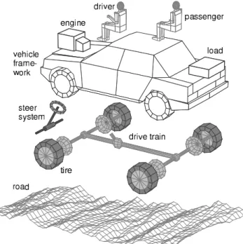
For dynamic simulation the vehicles are usually modeled by multi body systems (MBS), van der Jagt (2000). Typically, the overall vehicle model is separated into different subsystems, Rauh (2003). Fig. 1 shows the components of a passenger car model which can be used to investigate handling and ride properties. The vehicle model consists of the vehicle framework and subsystems for the steering system and the drive train. 1
The vehicle framework represents the kernel of the model. It at least includes the module chassis and modules for the wheel/axle suspension systems. The vehicle framework is supplemented by modules for the load, an elastically suspended engine, and passenger/seat models. A simple load module just takes the mass and inertia properties of the load into account. To describe the sloshing effects of liquid loads dynamic load models are needed, Rill and Rauh (1992). The subsystems elastically suspended engine, passenger/seat, and in heavy truck models a suspended driver’s cabin can all be handled by the presented generic free body model. For standard vehicle dynamics analysis the chassis can be modeled by one rigid body. For applications where the chassis flexibility has to be taken into account a suitable flexible frame model is presented. Most wheel/axle suspension systems can be described by typical multi body system elements such as rigid bodies, links, joints and force elements, Rill (1994). Using a modified implicit Euler algorithm for solving the dynamic equations, axle suspensions with compliancies and dry friction in the damper element can be handled without any problems, Rill (2004). Due to their robustness leaf springs are still a popular choice for solid axles. They combine guidance and suspension properties which causes many problems in modeling, Fickers and Richter (1994). A leaf spring model is presented in this paper which overcomes these problems.
The steering system at least consists of the steering wheel, a flexible steering shaft, and the steering box which may also be power-assisted. Neureder (2002) has developed a very sophisticated model of the steering system which includes compliancies, dry friction, and clearance.
Presented at XI DINAME – International Symposium on Dynamic Problems of Mechanics, February 28th - March 4th, 2005, Ouro Preto. MG. Brazil. Paper accepted: June, 2005. Technical Editors: J.R.F. Arruda and D.A. Rade.
Figure 1. Vehicle model structure.
Tire forces and torques have a dominant influence on vehicle dynamics. The semi-empirical tire model TMeasy has mainly been developed to meet both the requirements of user-friendliness and sufficient model accuracy, Hirschberg et. al. (2002). Complex tire models such as the FTire Model provided by Gipser (1998) can be used for special applications. The module tire also includes the wheel rotation which acts as input for the drive train model. The presented drive train model is generic. It takes lockable differentials into account, and it combines front wheel, rear wheel and all wheel drive. The drive train is supplemented by a module describing the engine torque. It may be modeled quite simply by a first order differential equation or by the enhanced engine torque module en-DYNA developed by TESIS.
Road irregularities and variations in the coefficient of friction present significant impacts on the vehicle. A road model generating a two-dimensional reproducible random profile was provided by Rill (1990).
Module Flexible Frame
Multi Body Approach to First Eigenmodes
The chassis eigenmodes of most passenger cars start at f >20Hz. Hence, for standard vehicle dynamic analysis the chassis can be modeled as one rigid body. The lower chassis stiffness of trucks and pickups results in eigenmodes starting at f ≈10Hz, Fig. 2.
Figure 2. Chassis eigenmode of a pickup at f=11.2 Hz.
The first eigenmodes consist of torsion and bending of the chassis. These modes can be approximated by a multi body chassis model where the chassis is divided into three parts, Fig. 3.
Figure 3. Flexible frame model.
Free Body Motions
The position and orientation of the reference frame x , C y , C z C which is fixed to the center body with respect to the inertial frame
0
x , y0, z0 is given by the rotation matrix
0C 0C 0C 0C
0C 0C 0C
0C 0C
0C 0C
0C 0C
cos -sin 0 cos 0 sin
A = sin cos 0 0 1 0
0 0 1 -sin 0 cos
0 0 0
0 cos -sin
1 sin cos
γ γ β β
γ γ
β β
α α
α α
× ×
×
(1)
and the position vector
0
0 0 0
0 C
C C
C
x
r y
z
,
= , (2)
where the comma separated subscript 0 indicates that the coordinates of the vector from 0 to C are expressed in the inertial frame. The generalized coordinates roll, pitch, and yaw angle α0C,
0C
β , γ0C as well as the coordinates x0C, y0C, z0C of the vector
0C0
r , describe the free body motion of the vehicle.
Modal Coordinates
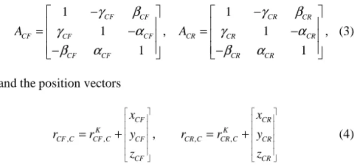
The motions of the front and rear body relative to the center body are small compared to the free body motions of the center part. Hence, the linearized rotation matrices
1 1
1 1
1 1
CF CF CR CR
CF CF CF CR CR CR
CF CF CR CR
A A
γ β γ β
γ α γ α
β α β α
− −
= − , = − ,
− −
(3)
and the position vectors
CF CR
K K
CF C CF C CF CR C CR C CR
CF CR
x x
r r y r r y
z z
, , , ,
= + , = + (4)
are used to describe the orientation and position of the front and rear body relative to the center part. The vectors K
CF C
r , and rCR CK, denote
the initial position of the front and rear body. The generalized coordinates
[
]
[
]
T
F CF CF CF CF CF CF
T
R CR CR CR CF CR CR
y x y z
y x y z
α β γ
α β γ
= , , , , , ,
= , , , , (5)
describe the motions of the front and rear body relative to the center body. These motions are approximated by n eigenmodes M e , 1 e , 2
... ,
M
n
e now
1
2
1 2
1
2
1 2
, ...
, ...
=
=
⋮
⋮
F F F FnM
E f
nM
F F R RnM
ER
nM m m
y e , e e
m
m m
y e , e e
m
(6)
where m1, m2, ...,
M
n
m are modal coordinates, and EF and ER
represent 6×nM matrices containing the eigenmodes.
Generalized Coordinates
The flexible chassis is modeled by 3 rigid bodies here. The orientation and the position of the bodies are described by free body motions and modal coordinates
[
]
TnM C
C x m m m
y = 0 Z0Cα0Cβ0Cγ0C 1 2… (7)
where the 6 free body motions and the nM modal coordinates are collected in the vector yC. The dimension of yC depends on the
number nM of modal coordinates, ny= +6 nM.
Equations of Motion
m rigid bodies it results in a set of two first order differential equations
K y z
M z q
= ,
= .
ɺ
ɺ (8)
The kinematic matrix K follows from the definition of the generalized speeds. The elements of the mass matrix M are given by
0 0 0 0
1
T T
m
k k k k
ij k k
k i j i j
v v
M m
z z z z
ω ω
=
∂ ∂ ∂ ∂
= + Θ ,
∂ ∂ ∂ ∂
∑
(9)where mk is the mass and Θk the inertia tensor of body k . Finally, the components of the generalized forces and torques are defined by
0 0
0 0 0 0
1
T T
n
R R
k k
i Ak k k Ak k k k k k
k i i
v
q F m a T
z z
ω α ω ω
=
∂ ∂
= − + − Θ − × Θ ,
∂ ∂
∑
(10)where F , Ak T denote the forces and torques applied to body Ak k
and 0 R k
a , 0
R k
α are remaining parts of the accelerations which do not depend on the derivatives of the generalized speeds.
Applied Forces and Torques
The forces and torques applied to the bodies can be written as
ext cmp cmp
C C CF CR
ext cmp
F F CF
ext cmp
R R CR
F F F F
F F F
F F F
= + + ,
= − ,
= −
(11)
and
ext cmp cmp
C C CF CR
ext cmp
F F CF
ext cmp
R R CR
T T T T
T T T
T T T
= + + ,
= − ,
= − ,
(12)
where the superscripts ext and cmp denote external and
compliance forces and torques.
Applying Jordain’s Principle, one part within the equations of motion describes the whole chassis motion. The compliance forces and torques are internal forces for the whole chassis and, therefore, do not show up in the corresponding parts of the generalized force vector.
If we assume that the compliance forces and torques are proportional to the motions of the front and rear body then, we will get
and
cmp cmp
CF CR
CF F CR R
cmp cmp
CF CR
F F
c y c y
T T
= = , (13)
where cCF and cCR mark 6 6× stiffness matrices. The modal coordinate approximation Eq. 6 results in
1 1
2 2
and
cmp cmp
CF CR
CF F CR R
cmp cmp
CF CR
nF nF
m m
m m
F F
c E c E
T T
m m
= = .
⋮ ⋮ (14)
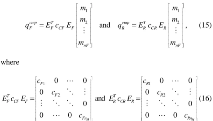
Within Jordain’s Principle the compliance forces and torques are reduced to generalized forces which are calculated by
1 1
2 2
and
cmp T cmp T
F F CF F R R CR R
nF nF
m m
m m
q E c E q E c E
m m
= = ,
⋮ ⋮ (15)
where
1 1
2 2
0 0 0 0
0 0
and
0 0
0 0 0 0
= =
⋯ ⋯
⋱ ⋮ ⋱ ⋮
⋮ ⋱ ⋱ ⋮ ⋱ ⋱
⋯ ⋯
M M
F R
F R
T T
F CF F R CR R
Fn Rn
c c
c c
E c E E c E
c c
(16)
are nM×nM stiffness matrices. which are defined by the modal
stiffnesses cF1, cF2, ... cFnM and cR1, cR2, ... cRnM. Thus, to
describe the motions of a flexible chassis only some eigenmodes and modal stiffnesses have to be provided.
Results
Depending on the vehicle layout, a flexible frame has a significant influence on the driving behavior, Fig 4. The rear axle of the considered bus is guided by four links. Here, the arrangement of the links generates a steering effect which depends on the roll angle of the rear part of the chassis and, therefore, also on the torsional stiffness of the chassis.
Module Leaf Spring
Modeling Aspects
Poor leaf spring models approximate guidance and suspension properties of the leaf spring by rigid links and separate force elements, Matschinsky (1998). The deformation of the leaf springs must be taken into account for realistic ride and handling simulations.
Within ADAMS leaf springs can be modeled with sophisticated beam-element models, ADAMS/Chassis 12.0. But, according to Fickers (1994) it is not easy to take the spring pretension into account. To model the effects of a beam, ADAMS/Solver uses a linear 6 -dimensional action-reaction force (3 translational and 3 rotational) between two markers. In order to provide adequate representation for the nonlinear cross section, usually 20 elements are used to model one leaf spring. A subsystem consisting of a solid axle and two beam-element leaf spring models would have
6 2 (20 6) 246
f = + ∗ ∗ = degrees of freedom. In addition, the beam-element leaf spring model results in extremely stiff differential equations. These and the large number of degrees of freedom slow down the computing time significantly.
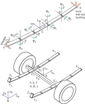
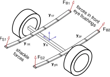
For real time applications the leaf springs must be modeled by a simple, but still accurate model. Fig. 5 shows a model of a solid axle with leaf spring suspension, which is typical for light truck rear axle suspension systems. There are no additional links. Hence, only the forces and torques generated by leaf spring deflections guide and suspend the axle.
Y
C
X
Z
P Q
S R
ϕ3
ψ3
ϕ4
ψ4
ϕ1
ψ1
ϕ2
ψ2
front leaf eye bushing
shac kle
xL zL yL
B xB
zB
yB
x, y, z α, β, γ Y1
C1
X1
Z2
Y2
Z1
X2
A CA
xA
zA
yA
C2
Figure 5. Axle model with leaf spring suspension.
The position of the axle center A and the orientation of an axle fixed reference frame x , A y , A z are described relative to a chassis A
fixed frame x , B y , B z by the displacements B ξ, η, ζ and the rotation angles α, β, γ which are collected in the 6 1× axle position vector
[
]
TA
y = , , , , ,ξ η ζ α β γ . (17)
Similar to Fickers (1994) each leaf spring is modeled by five rigid bodies which are connected to each other by spherical joints, Fig. 5.
Each leaf spring is connected to the frame via the front leaf eye
X. Furthermore each leaf spring is attached to the shackle at Y , and again to the frame at Z . In C the center part of each leaf spring is rigidly connected to the axle. The front eye bushings are modeled by spring/damper elements in x -, y -, and z -direction. The shackles are modeled by radial and a lateral spring/damper elements. Within each leaf spring the angles ϕ1, ψ1, and ϕ2, ψ2
describe the motions of part P - Q and part R - S relative to the center part. The outer parts Q - X and P - Y perform their rotations, ϕ3, ψ3, and ϕ4, ψ4, relative to part P Q and part R
-S . As each leaf spring element is considered as a rigid rod, the roll
motions can be neglected. The angles are collected in 4 1× position vectors
(1) (1) (1) (1) (1) (1) (1) (1)
1 1 1 3 3 1 2 2 4 4
T T
F R
y =ϕ ψ ϕ ψ, , , ;y =ϕ ψ ϕ ψ, , , ; (18)
(2) ( 2) (2) ( 2) (2) ( 2) (2) ( 2)
2 1 1 3 3 2 2 2 4 4
T T
F R
y =ϕ ψ, ,ϕ ψ, ;y =ϕ ψ, ,ϕ ψ, ; (19)
where y1F, y2 F and y1R, y2 R describe the momentary shape of the
front and the rear part of the left (1) and the right (2) leaf spring. A fully dynamic description of a solid axle with two five link leaf spring models would result in f= + ∗ =6 2 8 22 degrees of freedom. Compared to the beam-element model this is a really significant reduction.
But a dynamic description of the five link leaf spring model still includes some high frequent modes which will cause problems in the numerical solution of the equations of motion. As mass and inertia properties of the leaf spring model parts are small compared to the solid axle, a quasi static solution of the internal leaf spring deflection should be accurate enough within the overall vehicle model.
A quasi static solution provides the position vectors of the leaf spring parts as functions of the axle position vector,
( )
1F 1F A
y =y y ,y1R=y1R
( )
yA ,y2F=y2F( )
yA ,y2R=y2R( )
yA . Hence,the subsystem solid axle with two leaf springs has only f =6 degrees of freedom.
Initial Shape and Pretension
At first it is assumed that the leaf spring is located in the xz -plane of the leaf spring fixed frame x , L y , L z and its shape in the L design position can be approximated by a circle which is fixed by the points X , C and Y . By dividing the arc X - Y into 5 parts of equal length the position of the links P , R , S , Q and the initial values of the angles ϕ01, ψ01, ϕ02, ψ02, ϕ03, ψ03, ϕ04, ψ04 can be
calculated very easily.
In design position each leaf spring is only preloaded by a vertical load which results in zero pretension forces in the y -L
direction, 0 0 y B
F = , 0 0
y S
F = and zero pretension torques around the
l
z -axis, 0 0
z P
T = , 0 0
z Q
T = , 0 0
z R
T = , 0 0
z S
T = . In addition the torques
around the x -axis vanish, l 0 0 x P
T = , T0xQ=0, 0 0 x R
T = , T0xS=0.
To transfer the vertical preload F to the front eye bushing and 0
the y -axis, Fig. 6. The pretension forces in the front eye bushing L
0 x B
F , 0
z B
F and in the shackle F , can easily be calculated from the 0S equilibrium conditions of the five link leaf spring model,
0 0
0 0 0
0 0 0
0 0 0
x x
B S YZ
z z
B S YZ
x z x x z
XC XY S YZ XY S YZ
F F u
F F F u
r F r F u r F u
+ = ,
+ + = ,
− + − = ,
(20)
Figure 6. Pretension forces and torques.
where u refers to the unit vector in the direction of the shackle, YZ
and x XY
r , z
XY
r are the x and z components of the vector from pointing from X to Y . The pretension torques in the leaf spring joints around the y -axis, L 0
y P
T , 0 y Q
T , 0y R
T , 0 y S
T follow from
0 0 0
0 0 0
0 0 0
0 0 0
0
0
0
0
y z x x z
P PX B PX B
y z x x
Q QX B QX Bz
y z x x z
R RY S YZ RY S YZ
y z x x z
S SY S YZ SY S YZ
T r F r F
T r F r F
T r F u r F u
T r F u r F u
− + − =
− + − =
+ − =
+ − =
(21)
where r , iij = , , ,P Q R S, j= ,X Y are vectors pointing from i to
j.
Compliance
The leaf spring compliance is defined in the design position by
the vertical and the lateral stiffness,
c
V andc
L. In Fig. 7a the leaf spring is approximated by a beam which is supported on both ends and is loaded in the center by the force F .Figure 7. Leaf spring stiffness.
The deflection w and the force F are related to each other via the stiffness c
F=c w. (22)
If we transfer the beam model to the five link leaf spring model and look at the front half, Fig. 4, one will get
w=aϕ1+a
(
ϕ ϕ1+ 3)
, (23)where a defines the length of one link, and small deflections in the
L
x , z plane were assumed. The torques around the L y -axis in the L joints P and Q are proportional to the deflection angles ϕ1 and ϕ3
1 1 and 3 3
y y
P Q
T =cϕϕ T =cϕϕ . (24)
The equilibrium condition results in
2 and
2 2
y y
P Q
F F
T = a T =a : . (25)
The leaf spring bending mode due to a single force can be approximated very well by a circular arc. Hence, the relative angle between connected links is equal, ϕ1=ϕ3=ϕ and Eq. 23 can be
simplified to w=3aϕ or or ϕ = a w
3 . From Eqs. 24 and 25 follows
13 2 2 and 33 2
w F w F
c a c a
a a
ϕ = ϕ = . (26)
Using Eq. 22, one finally obtains
1 3
2 3 2
3 and
2
V V
cϕ = a c cϕ = a c , (27)
where the beam stiffness
c
was replaced by the vertical leaf spring stiffness c . Assuming symmetry, the stiffnesses in the rear joints Vare given by cϕ2 =cϕ1 and cϕ4=cϕ3. The stiffnesses around the
vertical axis 1
cψ , 2
cψ , 3
cψ and 4
cψ can be calculated in a similar
way. The torsional stiffness of the leaf spring is neglected in this approach.
Actual Shape
The energy of a flexible system achieves a minimum value,
Min
E→ , in an equilibrium position. The energy of the five link leaf spring model is given by
1 1 3 3
2 2 4 4
2 2 2 2
1 1 3 3
2 2 2 2 2 2
2 2 4 4
1 1 1 1 1
2 2 2 2 2
1 1 1 1 1 1
,
2 2 2 2 2 2
T X B X
SR SR SL SL
E w c w c c c c
c c c c c w c w
ϕ ψ ϕ ψ
ϕ ψ ϕ ψ
ϕ ψ ϕ ψ
ϕ ψ ϕ ψ
= + + + + +
+ + + + + +
(28)
where w is the 3 1X × displacement vector and c is the 3 3B ×
According to Eqs. 18 and 19, the actual shape of the leaf spring
is determined by the position vectors 1
[
1 1 3 3]
Ty = ϕ ψ ϕ ψ, , , and
[
]
2 2 2 4 4 T
y = ϕ ψ ϕ ψ, , , . If the leaf spring energy becomes a
minimum, the following equations will hold
1 1 4 4
0 0 0 0
E E E E
ϕ ψ ϕ ψ
∂ = , ∂ = , ∂ = , ∂ = .
∂ ∂ ⋯ ∂ ∂ (29)
As the shackle displacements w , SR wSL do not depend on y 1
and the front bushing displacement vector w does not depend on X
2
y the conditions in Eq. 29 form two independent sets of nonlinear
equations f y y1( 1, A)=0 and f y y2( 2, A)=0, where y denotes the A dependency of the actual position and orientation of the solid axle. These equations are solved iteratively by the Newton-Algorithm. Starting with initial guesses 0
1
y , 0 2
y one gets an improvement by
solving the linear equations
1 1
1 1 1 1
1
1 2
2 2 2 2
2
( )
0 1 2
( )
k k
A
k k
A
f
y y f y y
y
k f
y y f y y
y
+
+
∂ − = −
∂
= , , ,...
∂ − = −
∂
(30)
Here, the Jacobians 1 1 f y
∂
∂ 22
f y
∂
∂ can be calculated analytically.
Leaf Spring Reaction Forces
The actual forces in the front leaf eye bushing are given by
0 X
B B B X B
F =F +c w +d uɺ , (31)
where F0B denotes the pretension force and
c
B, d are 3 3B × matrices, characterizing the stiffness and damping properties of the front leaf eye bushing. The displacement vector w in the front leaf Xeye bushing depend on the generalized coordinates y and 1 y A which describe the actual shape of the front leaf spring part and the actual position and orientation of the solid axle. By solving Eq. 30,
1
y is given as a function of y . Hence, A w only depends on x y A and its derivative can be determined by
X
X A
A
w y u
y
∂
= ,
∂ ɺ
ɺ (32)
where yɺA describes the velocity state of the solid axle.
The radial and lateral components of the shackle forces can be calculated from
0 and 0
= T + + ɺ = T + + ɺ ,
SR SL
SR SR S SR SR SR SL SL S SL SL SL
F u F c w d w F u F c w d w (33)
where F represents the pretension force, 0S u , SR u are unit vectors SL
in the radial and lateral shackle direction, and cSR, cSL, dSR, dSL are constants characterizing the stiffness and damping properties of the shackle. The shackle displacements w and SR wSL depend on the
generalized coordinates y2 R and y which describe the actual A shape of the rear leaf spring part and the actual position and
orientation of the solid axle. Similarly to Eq. 32 the displacement velocities are given by
and
SR SL
SR A SL A
A A
u u
y y
u u
y y
∂ ∂
= = .
∂ ɺ ∂ ɺ
ɺ ɺ (34)
Finally, the shackle force reads as
FS=F uSR SR+F uSL SL. (35)
Forces Applied to the Axle
The leaf springs act like generalized force elements in this approach, Fig. 8. Guidance and suspension of the solid axle is done by the resulting force
1 2 1 2
B B S S
F=F +F +F +F (36)
and the resulting torque
1 1 2 2 1 1 2 2
AB B AB B AS S AS S
T=r ×F +r ×F +r ×F +r ×F , (37)
where rAB1=rAB1(yA), ... rAS2(yA) describe the momentary position of the front eye bushings and the shackles relative to the axle center.
Figure 8. Forces applied to the axle.
As the forces in the front eye bushings F , B1 FB2 and the
shackle forces F , S1 F depend on the axle state S2 y , A yɺA only, the
resulting force F and the resulting torque T are also functions of the axle state only. Since, hereby each leaf spring acts as a generalized force element, it can easily be integrated into the vehicle framework. By suppressing high frequent leaf spring eigenmodes, it is perfectly adopted to real-time application.
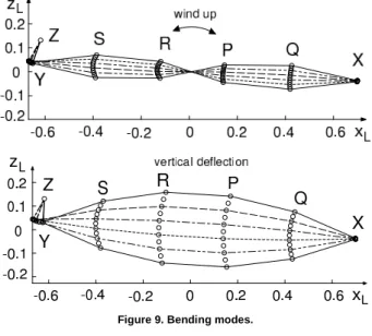
Bending Modes
Figure 9. Bending modes.
Model Performance
The five link leaf spring model was integrated into a ve-DYNA Ford Transit vehicle model.
Figure 10. Comparison to measurements.
Using this model at the rear axle instead of a poor kinematic approach means only 85% more computer run time. Hence, real time applications are still possible. The simulation results are in
good conformity to measurements, Fig. 10. The nonlinearity in the spring characteristics is caused by an additional bump stop and by the change of the shackle position during jounce and rebound. Obviously, the five link model is accurate enough.
Free Body Module
Position and Orientation
To describe the momentary state of the body E the frame x E
E
y , z located in the center of gravity is used. In addition, sensor E points S monitor position, velocity, and acceleration at specific body points, Fig. 11.
Figure 11. Elastically suspended body.
The frame B is fixed to the vehicle. The suspension of body E on the vehicle, frame B may consist of force elements and/or rubber mounts. The road-fixed frame 0 is considered as an inertial frame. The position of frame B with respect to the road-fixed inertial frame 0 is given by the position vector
0 0 B
B B
B
x
r y
z
,
= . (38)
The orientation of the frame axes is described by a rotation matrix. Three elementary rotations are put together. The sequence
0
yaw pitch roll
B B
B
B
A = Aγ Aβ Aα
(39)
results in
[
B B]
B
A0 = cosβ cosγ
+ +
+ +
=
B B B
B B
B B B B
B B B B
B B B
B
B B B B
B B
B B B B
B
B
α
α
α
A
β α β
α β
γ β α γ
β α γ β
γ γ
γ β α γ
β α
γ γ
α γ α γ β
cos cos cos sin sin
-cos sin cos cos sin sin cos cos
cos sin cos cos
cos sin cos cos sin sin
sin sin sin sin sin cos cos
cos B B B
Hence, position and orientation of the vehicle-fixed reference frame are described by 6 generalized coordinates x y zB, ,B B and
B B B
α β γ, , .
The position and orientation of the elastically suspended body with respect to the reference frame B is defined by
E BE B E E x r y z ,
= . (41)
and
1 0 0 cos 0 sin
0 cos sin 0 1 0
0 sin cos sin 0 cos
cos sin 0
sin cos 0
0 0 1
E E
BE E E
E E E E
E E
E E
A
β β
α α
α α β β
γ γ γ γ = − × × − − × − . (42) Generalized Speeds
The velocity of the reference frame B with respect to the inertial frame 0 is given by
0 0 0 0 B B
B B
B
x
v r y
z , , = = ɺ ɺ ɺ ɺ (43)
The velocity denoted in the inertial frame can be transformed to the reference frame
0 0 0 0
T B
B B B
v , =A rɺ , . (44)
By this, the orthogonality of the rotation matrix
1
0 0 0
T
B B B
A =A− =A (45)
was already taken into consideration.
The angular velocity of the reference frame B with respect to the inertial frame 0 may be expressed directly in reference frame
B
0
1 0 sin
0 cos sin cos
0 sin cos cos
B B
B B B B B B
B B B B
β α
ω α α β β
α α β γ
, − = . − ɺ ɺ ɺ (46)
The 6 components of v0B B, and ω0B B, will be chosen as
generalized speeds now. First order kinematical differential equations connect this speeds with the derivatives of the
0 0 0 0 B Bx B By B B Bz v x A v y v z = ɺ ɺ ɺ (47) and 0 0 0
1 0 sin
0 cos sin cos
0 sin cos cos
B
B Bx
B B B B By
B B B B Bz
β α ω
α α β β ω
α α β γ ω
− = , − ɺ ɺ ɺ (48)
where the solution of Eq. 48 is given by
0 0
0 0
0
( cos sin ) cos
sin cos
cos
Bz B By B B
B
Bz B By B
B
B Bx B B
ω α ω α β
γ
ω α ω α
β
ω γ α
α = + / , = − + , = + . ɺ ɺ ɺ ɺ (49)
The momentary state of the reference frame B is fully characterized by 6 generalized coordinates x y zB, , , , ,B B α β γB B B
and 6 generalized speeds v0Bx,v0By,v0Bz,ω ω ω0Bx, 0By, 0Bz.
The velocity and the angular velocity of the elastically suspended body with respect to the inertial frame 0 is given by
0 0 0
0 0
BE B
E B B B B B BE B
E B B B BE B
v v ω r r
ω ω ω
, , , , , , , , = + × + , = + , ɺ (50)
where the derivative of the position vector and the angular velocity of the elastically suspended body follow from the Eqs. 41 and 42. They read as
E
BE B E
E x y r z , = ɺ ɺ ɺ ɺ (51) and
1 0 sin
0 cos sin cos
0 sin cos cos
E E
BE B E E E E
E E E E
β α
ω α α β β
α α β γ
, = − . ɺ ɺ ɺ (52)
By using the components of the velocity
0 0
0 0x y z
T
E E
E B E
v v v v
, = (53)
and the angular velocity
0 0
0 0x y z
T
E E
E B E
ω ω ω ω
, = (54)
as generalized speeds, Eq. 50 can be written as a set of kinematical differential equations
0 0 0
0 0 0
0 0 0
x x x
y y y
z z z
E B E
E E
E B E E
E
E E B E E
v v x
x
v v y
y
z
z v v
ω ω ω − = − − × − ɺ ɺ ɺ (55) and 0 0 0 0 0 0
1 0 sin
0 cos sin cos
0 sin cos cos
x x y y z z E B E E E B
E E E E
E E E E E B
ω ω
β α
α α β β ω ω
α α β γ ω ω
− − = − . − ɺ ɺ ɺ (56)
B, the 6 generalized speeds v0Ex,v0Ey,v0Ez,ω ω ω0Ex, 0Ey, 0Ez are the
components of the absolute velocity and angular velocity of body
E .
Accelerations
The accelerations of body E with respect to the inertia frame 0 can be expressed in reference frame B . They read as
0
0 0 0
0
0 0 0
E B
E B B B E B
E B
E B B B E B
a v ω v
α ω ω ω
,
, , ,
,
, , ,
= + × ,
= + × ,
ɺ
ɺ (57)
where
0 0x 0 y 0 z
T
E B E E E
vɺ , =vɺ vɺ vɺ (58)
and
0 0 x 0 y 0z
T
E B E E E
ωɺ , =ωɺ ωɺ ωɺ (59)
follow from the Eqs. 53 and 54.
Force Elements
If a force element is attached to the chassis at point i and to the body at point j , the momentary position of force element ij will
be defined by
ij B BE B Ej B Bi K
Bj B
r r r r
r
, , , ,
,
= + − , (60)
where
Ej B BE Ej K
r , =A r , , (61)
Bi K
r , , rEj K, are given by data, and rBE B, follows from Eq. 41. The
actual length can be calculated from
a T
ij ij B ij B
u = r, r, , (62)
and the unit vector
ij B ij B a ij
r e
u
,
, = (63)
describes the momentary direction of the force element. If 0 ij
u
denotes the initial length of the force element, the displacement of the force element will be formed by
0 a ij ij ij
u =u − .u (64)
The displacement velocity follows from
T ij ij B ij B
d
v e r
dt
, ,
= . (65)
Using Eq. 60, Eq. 61, and rɺBi K, =0 one gets
T BE B
ij ij B BE B ej B
v e, r , ω , r,
= ɺ + × , (66)
where rɺBE B, and ωBE B, are given by the Eqs. 51 and 52. The forces
ij B
F, , Fji B, and the torques Tij B, , Tji B, applied to body and chassis are determined by
ij B ij ij ij B ji B ij B
F, f u v e, F, F,
= , , = − , (67)
and
ij B Ej B ij B ji B Bi K ji B
T, =r , ×F, , T , =r , ×F, , (68)
where f describes an arbitrary spring/damper characteristic.
Equations of Motion
Applying liner and angular momentum to the elastically suspended body, one obtains
0E B 0 0
E E B E B B B E B
m vɺ , =F, −m g, +ω , ×v , (69)
and
0E B 0 0 0 0
E Bω TE B ωE B E BωE B E B ωB B ωE B
,
, , , , , , , ,
Θ ɺ = − × Θ − Θ × , (70)
where m , E ΘE B, denote mass and inertia tensor of the free body,
E B
F, , TE B, are the resulting forces and torques applied to the free
body, and g,B is the vector of gravity expressed in the body fixed
reference frame. These equations are coupled with the chassis equations of motion only by the applied forces and torques. Due to the particular choice of generalized speeds, no mass or inertia coupling terms appear.
By using this modeling technique, Seibert and Rill (1998) showed that the comfort of a passenger car is significantly influenced by the engine suspension system. The free body model can also be used to model an elastically suspended driver’s cab, Rill (1993).
Subsystem Drive Train
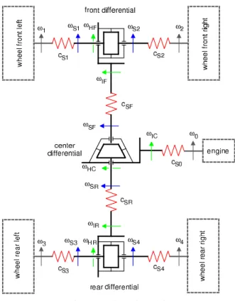
Generic Model Structure
The subsystem drive train, Fig. 12, interacts on one hand with the engine and on the other hand with the wheels. Hence, the angular velocities of the wheels ω1, …, ω4 and the engine or the
gear output angular velocity ω0 respectively are input quantities.
Figure 12. Drive train model.
The drive train model includes three lockable differentials. The angular velocities of the drive shafts ωS1: front left, ωS2: front
right, ωSF: front, ωSR: rear, ωS3: rear left, ωS4: rear right are used
as generalized coordinates.
The torque distribution of the front and rear differential is 1:1. If
F
r and r are the ratios of the front and rear differential, one will R get
1 2
1 1
2 2
HF S S
IF rF HF
ω ω ω
ω ω = + , = ; (71) 3 4 1 1 2 2
HR S S
IR rR HR
ω ω ω
ω ω
= + ,
= .
(72)
The torque distribution of the center differential is formed by
1 F R t t µ µ = , − (73)
where t , F t denote the torques transmitted to the front and rear R drive shaft, and µ is a dimensionless drive train parameter. A value of µ =1 means front wheel drive, 0< <µ 1 stands for all wheel drive, and µ =0 is rear wheel drive. If the ratio of the center differential is given by r then C
HC SF (1 ) SR
C HC
IC r
ω µω µ ω
ω ω
= + −
= (74)
holds.
Equation of Motion
The equation of motion for the drive train is derived from Jordain’s Principle, which reads as
(
Θiωi−ti)
δ ωi= ,0∑
ɺ (75)where Θi is the inertia of body i , ωɺi denotes the time derivative of the angular velocity, t is the torque applied to each body, and i δ ωi describe the variation of the angular velocity. Applying Eq. 75 for the different parts of the drive train model results in
(
)
(
)
(
)
1
1 1 1
2
2 2 2
front drive shaft left 0
front drive shaft right 0
front differential housing 0
front differential input shaft
S
S S LF S
S
S S LF S
HF HF HF IF IF t t t t δ ω ω δ ω ω δ ω ω ω
: Θ − − = ,
: Θ − + = ,
: Θ = ,
: Θ
ɺ ɺ
ɺ ɺ
(
+tSF)
δ ωIF= ,0(76)
(
)
(
)
(
)
front drive shaft 0
rear drive shaft 0
center differential housing 0
center differential input shaft
SF
SF SF LC SF
SR
SR SR LC SR
HC HC HC t t t t δ ω ω δ ω ω δ ω ω
: Θ − − = ,
: Θ − + = ,
: Θ = ,
: Θ
ɺ ɺ
ɺ
(
ICω +ɺIC tS0)
δ ωIC= ,0(77)
(
)
(
)
(
)
(
34 34 34)
34rear differential input shaft 0
rear differential housing 0
rear drive shaft left 0
rear drive shaft right
IR
IR SR IR
HR
HR HR
S
S S LR S
S
S S LR S
t t t t t δ ω ω δ ω ω δ ω ω δ ω ω
: Θ + = ,
: Θ = ,
: Θ − − = ,
: Θ − +
ɺ ɺ ɺ
ɺ = .0
(78)
Using the Eqs. 71, 74, and 72 one gets:
(
)
(
)
(
)
1
1 1 1
2
2 2 2
1 2 1 2
1 2 1 2
0 0
1 1 1 1
0
2 2 2 2
1 1 1 1
0
2 2 2 2
0 S
S S LF S
S
S S LF S
S S
HF S S
S S
IF F F SF F S F S
SF
SF SF LC SF
SR
SR SR
t t
t t
r r t r r
t t t δ ω ω δ ω ω
δ ω δ ω
ω ω
δ ω δ ω
ω ω δ ω ω ω
Θ − − = ,
Θ − + = ,
Θ + + = ,
Θ + + + = ,
Θ − − = ,
Θ − +
ɺ ɺ ɺ ɺ ɺ ɺ ɺ ɺ
(
)
(
)
(
)
(
)
(
)
0(
)
3 4 3 4
3 4
0
(1 ) (1 ) 0
(1 ) (1 ) 0
1 1 1 1
0
2 2 2 2
1 1 1
2 2 2
LC SR
SF SR
HC SF SR
SF SR
IC C C S C SF C SR
S S
IR R R SR R S R S
S S
HR
t
r r t r r
r r t r r
δ ω
µω µω µδ ω µ δ ω
µ ω µ ω µ δ ω µ δ ω
δ ω δ ω
ω ω δ ω ω ω = ,
Θ + − + − = ,
Θ + − + + − = ,
Θ + + + = ,
Θ + ɺ ɺ ɺ ɺ ɺ ɺ ɺ ɺ
(
)
(
)
3 4 33 3 3
4
4 4 4
1 0 2 0 0 S S S
S S LR S
S
S S LR S
t t t t δ ω δ ω ω δ ω ω + = ,
Θ − − = ,
Θ − + = .
ɺ ɺ
(79)
Collecting all terms with δ ωS1, δ ωS2, δ ωSF , δ ωSR, δ ωS3,
4 S
δ ω and using the abbreviations ν= −1µ, 2 HF HF rF IF ∗
Θ = Θ + Θ ,
2 HC HC rC IC ∗
Θ = Θ + Θ , and 2
HR HR rR IR ∗
Θ = Θ + Θ finally leads to three blocks of differential equations
1 2
1 1
1 2 2 2
1 1 1
4 4 2
1 1 1
4 4 2
S S
S HF HF S LF F SF
S S
HF S HF S LF F SF
t t r t
t t r t
ω ω ω ω ∗ ∗ ∗ ∗
Θ + Θ + Θ = + − ,
Θ + Θ + Θ = − − ,
ɺ ɺ
ɺ ɺ
2
0 2
0
SF SR
SF HC HC SF LC C S
SF SR
HC SR HC SR LC C S
t t r t
t t r t
µ ω µν ω µ
µν ω ν ω ν
∗ ∗ ∗ ∗
Θ + Θ + Θ = + − ,
Θ + Θ + Θ = − − ,
ɺ ɺ
ɺ ɺ
(81)
3 4
3 3
3 4 4 4
1 1 1
4 4 2
1 1 1
4 4 2
S S
S HR HR S LR R SR
S S
HR S HR S LR R SR
t t r t
t t r t
ω ω ω ω ∗ ∗ ∗ ∗
Θ + Θ + Θ = + − ,
Θ + Θ + Θ = − − ,
ɺ ɺ
ɺ ɺ
(82)
which describe the dynamics of the drive train. Due to its simple structure, an extension to a 6x6 or 8x8 drive train will be straight forward.
Drive Shaft Torques
The torques in the drive shafts are given by
1 1 1 1 1 1
2 2 2 2 2 2
0 0 0 0 0
3 3 3 3 3 3
4 4 4
where where where where where where where
S S S S S
S S S S S
SF SF SF SF IF SF
S S S S IC
SR SR SR SR IR SR
S S S S S
S S S
t c t c t c t c t c t c t c
ϕ ϕ ω ω
ϕ ϕ ω ω
ϕ ϕ ω ω
ϕ ϕ ω ω
ϕ ϕ ω ω
ϕ ϕ ω ω
ϕ = , : = − ; = , : = − ; = , : = − ; = , : = − ; = , : = − ; = , : = − ; = , : △ △ △ △ △ △ △ △ △ △ △ △
△ △ϕS4 = ω ω4− S4;
(83)
and cS0, c , S1 cS2, cS3, cS4, cSF, cSR denote the stiffnesses of the drive shafts. The first order differential equations can be arranged in matrix form
0
K
ϕɺ= ω+ Ω ,
△ (84)
where
1 2 3 4
T
S S SF SR S S
ω ω ω ω ω ω ω
= , , , , , (85)
represents the vector of the angular velocities,
1 2 0 3 4
T
S S SF S SR S S
ϕ ϕ ϕ ϕ ϕ ϕ ϕ ϕ
= , , , , , ,
△ △ △ △ △ △ △ △ (86)
contains the torsional angles in the drive shafts,
0 1 2 0 0 0 3 4
T
ω ω ω ω ω
Ω = , , , − , , , (87)
is the excitation vector, and
1 0 0 0 0 0
0 1 0 0 0 0
1 1
1 0 0 0
2 2
0 0 0 0
1 1
0 0 0 1
2 2
0 0 0 0 1 0
0 0 0 0 0 1
F F
C C
R R
r r
K r r
r r µ ν − − − = − − − (88)
forms a 7x6 distribution matrix.
Locking Torques
The differential locking torques are created by an enhanced dry friction model consisting of a static and a dynamic part
S D
LF LF LF
S D
LC LC LC
S D
LR LR LR
t t t
t t t
t t t
= + ,
= + ,
= + .
(89)
The dynamic parts are modeled by a torque proportional to the differential output angular velocities
(
)
(
)
(
)
2 1 4 3 DLF LF S S
D
LC LC SR SF
D
LR LR S S
t d t d t d ω ω ω ω ω ω = − , = − , , = − (90)
where dLF, dLC, dLR are damping parameters which have to be chosen appropriately. In steady state operating conditions, the static parts S
LF
t , S LC
t , S LR
t will provide torques, even if the differential output angular velocities are equal. From the Eqs. 80, 81, and 82, one gets
(
)
(
)
(
)
2 1 0 4 3 1 2 1 (2 1) 2 1 2 DLF S S
D
LF SR SF C S
D
LR S S
t t t
t t t r t
t t t
µ
= − ,
= − + − ,
= − .
(91)
By this locking torque model, the effect of dry friction inside the differentials can also be taken into account.
Numerical Solution
The equations of motion 80, 81, and 82 can be combined in a matrix differential equation
( )
Mωɺ=q△ϕ ω, , (92)
where ω, △ϕ are given by the Eqs. 85, 86, and the mass matrix M is built by three 2x2 submatrices
0 0 0 0 0 0 F C R M M M M
= , (93)
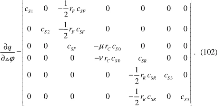
where the elements of M , F M , and C M follow from the Eqs. 80, R 81, and 82. The vector of the generalized torques is written as
1 2 0 0 3 4 1 2 1 2 (1 ) 1 2 1 2
S LF F SF
S LF F SF
SF LC C S
SR LC C S
S LR R SR
S LR R SR
t t r t
t t r t
t t r t
q
t t r t
t t r t
t t r t