ISSN 0101-8205 / ISSN 1807-0302 (Online) www.scielo.br/cam
Numerical solution of the variational PDEs
arising in optimal control theory
VICENTE COSTANZA1∗, MARIA I. TROPAREVSKY2 and PABLO S. RIVADENEIRA1,3
1Grupo de Sistemas No Lineales, INTEC, CONICET-UNL, Santa Fé, Argentina 2Departamento de Matemática, Facultad de Ingeniería, UBA, Buenos Aires, Argentina
3IRCCyN, 1 Rue de la Noë, 44321 Nantes Cedex 03, France
E-mails: [email protected] / [email protected] / [email protected]
Abstract. An iterative method based on Picard’s approach to ODEs’ initial-value problems
is proposed to solve first-order quasilinear PDEs with matrix-valued unknowns, in particular, the recently discovered variational PDEs for the missing boundary values in Hamilton equations of optimal control. As illustrations the iterative numerical solutions are checked against the ana-lytical solutions to some examples arising from optimal control problems for nonlinear systems and regular Lagrangians in finite dimension, and against the numerical solution obtained through standard mathematical software. An application to the(n+1)-dimensional variational PDEs associated with then-dimensional finite-horizon time-variant linear-quadratic problem is dis-cussed, due to the key role the LQR plays in two-degrees-of freedom control strategies for non-linear systems with generalized costs.
Mathematical subject classification: Primary: 35F30; Secondary: 93C10.
Key words:numerical methods, first-order PDEs, nonlinear systems, optimal control,
Hamil-tonian equations, boundary-value problems.
1 Introduction
Hamilton’s canonical equations (HCEs) are key objects in optimal control theory when convexity is present. If the problem concerning an n -dimensional con-trol system and an additive cost objective is regular, i.e. when the Hamiltonian
H(t,x, λ,u)of the problem is smooth enough and can be uniquely optimized with respect touat a control valueu0(t,x, λ)(depending on the remaining vari-ables), then HCEs appear as a set of 2nfirst-order ordinary differential equations whose solutions are the optimal state-costate time-trajectories.
In the general nonlinear finite-horizon optimization set-up, allowing for a free final state, the cost penaltyK(x)imposed on the final deviation generates a two-point boundary-value situation. This often leads to a rather difficult numerical problem. In the linear-quadratic regulator (LQR) case there exist well-known methods (see for instance [3, 19]) to transform the boundary-value into a final-value problem, giving rise to the differential Riccati equation (DRE).
For a quadratic K(x), in this paper it will always be K(x) = skxk2, the
implementing two-degrees-of-freedom (2DOF) control in the Hamiltonian con-text (see [15]), because the P˜(t) enters the compensation gain of the control scheme, and it can be obtained on-line from knowledge of P˜(0)(see [4, 9]).
When the variational PDEs were solved using standard software as MAT-LABr or MATHEMATICAr, some inaccuracies have appeared, which has made it necessary to develop robust integration methods. In this work, a novel iterative scheme based on Picard’s approach to ODEs’ initial-value problems is proposed to numerically integrate these variational PDEs. This convergent iterative method actually applies to general first-order quasilinear PDEs of the form
n X
i=1
ai(x,z) ∂z ∂xi =
b(x,z), (1)
wherex ∈Rn, zis the unknown real function ofx, and the{ai,i =1, . . . ,n;b}
areC1functions. The ‘Cauchy problem’ is to find theC1function (denoted for
simplicity z(x)) that satisfies Eq. (1) in a neighborhood of a given C1 ‘initial hypersurface’S⊂Rnwhere the ‘initial data’ are prescribed, i.e.
z(x)=g(x)∀x ∈S, (2)
for a givenC1functiong
:S→R.
the McLaurin series reached in each iteration. It is shown that this new method actually applies to first-order quasilinear PDEs with matrix-valued unknowns. As illustrations the iterative method is checked against: (i) the analytical so-lutions to examples in dimension one and higher, some arising from optimal control problems for nonlinear systems and regular Lagrangians, and (ii) the numerical solution obtained from straightforward use of standard mathematical software. An application to the(n+1)-dimensional variational PDEs associ-ated with then-dimensional finite-horizon time-variant linear-quadratic problem is specially discussed due to its relation to 2DOF control strategies for non-linear systems with generalized costs.
The paper is organized as follows: In Section 2, the proposed method for solving quasilinear PDEs is substantiated. The PDEs for boundary conditions of the Hamilton canonical equations are introduced in Section 3. A solution to these equations by means of the proposed iterative scheme is also included. In Section 4 some examples are discussed and illustrated. Finally, the conclusions are presented.
2 An iterative method for first-order quasilinear PDEs
Let us consider first-order quasilinear PDEs of the form given in Eq. (1) and its related Cauchy problem. Under the usual hypothesis thatSis non-characteristic, i.e., the vector(a1(x,g(x)),a2(x,g(x)) . . . ,an(x,g(x)) is not tangential to S
at anyx ∈ S, there exists a uniqueC1 solutionz(x)of Eq. (1), defined on a neighborhood ofS(see [13] for details). The graph of z(x)is the union of the parametric family of integral curves of
∂xi
∂t (v,t)=ai(x,y) , xi(v,0)=hi(v) (3) ∂y
∂t(v,t)=b(x,y) , y(v,0)=g(h(v)) (4)
wherevis a vector-parameter running alongS, i.e.Sis assumed to be given in parametric form
x ∈S⇒x =h(v) , (5)
For each value ofvthe Eqs. (3-4) are actually ODEs with independent variable
t. Then the Cauchy problem for the original quasilinear PDEs is basically an-swered by the theorem on existence and uniqueness of solutions for ODEs (see [14]), which in the positive case anticipates a uniqueC1solution(x(v,t),y(v,t))
for small|t|. TheC1 dependence of the ODE solutions in a bounded setOof
parametersv, guarantees that the solution curves are defined for|t| ≤t0for some
positivet0, i.e. uniformly, for allv∈O. In addition, sinceSis non-characteristic,
by the inverse-function theorem the function(v,t)→x(v,t)can be inverted in a neighborhoodofSto obtainvandtasC1functions ofxinso as to meet the initial condition
t(x)=0, h(v(x))=x , ∀x ∈S.
Therefore the desired solution to the original problem will be
z(x)= y(v(x),t(x)) , (6)
as can be checked by taking derivatives, using the chain rule and the matrix equality (see [13])
∂ (v,t) ∂x =
∂x ∂ (v,t)
−1 .
The problem remains formally the same when theai,i = 1, . . . ,n aren×n
-matrix-valued, andz,baren-vector-valued mappings.
For a fixedv, Eqs. (3-4) can be solved by using the Picard method for auto-nomous ODEs [14]. The extension of the Picard algorithm to treat Eqs. (3-4) as PDEs reads as follows.
For eachv0∈Owhere the functionx(v,t)is invertible, the ODE system (3-4) can be written
dY
dt = ˙Y = F(Y); (7) Yv0(0)=Y0(v0)=(h1(v0),h2(v0), . . . ,hn(v0),g(h(v0))), (8)
where Y def= (x1,x2, . . . ,xn,y) , F def= (a1,a2, . . . ,an,b), and F : Rn+1 → Rn+1isC1.
then the Picard sequence, for allt ∈ Jv0
def
= (−εv0, εv0)andv0fixed, is denoted
by{Yn(v0,∙), n=0,1, . . .}, and
Yn(v0,t)=(x1(v0,t), . . . ,y(v0,t))n =Y0+ Z
0 t
F(Yn−1(v0,s))ds, (9)
whereεv0 can be chosenεv0 < min n
1 Mv0,
1 Kv0
o
, where Kv0 is a Lipschitz
con-stant forF inB(v0) .
It is well-known that Picard iterations converge to the solution Y in some neighborhood oft = 0 whenever the solution to Eq. (7) exists and is unique, then by choosing a compact (as big as possible) set O0 ⊂ O, and using the
fact thatY0 is continuous, it follows thatW def
= S
v0∈O0 B(v0)is bounded, and
therefore there will exist a Lipschitz constant K, and a bound M for F in the closure ofW, with
K ≥ Kv0, M ≥Mv0 ∀v0∈O0. (10)
Then, it turns possible to choose an ε < minM1,K1 ensuring that Eq. (9) will be valid for all t ∈ J def= [−ε, ε] and for all v0 ∈ O0. Therefore, in the
compact setO0× J, the Picard sequenceYn(v0,∙)will converge uniformly to Y(v0,∙), the solution of the ODE (7), implying that the last coordinate yn(v0,t)
of Yn(v0,∙) will converge (uniformly) to y(v0,t) = z(x(v0,t)). By calling 0def= x(O0×J), the following proposition becomes true.
Proposition 2.1. Let consider a first-order PDE
n X
i=1
ai(x,z) ∂z ∂xi =
b(x,z) (11)
z(x)=g(x)x ∈ S (12)
where x ∈ Rn and S is an hypersurface in
Proposition 2.1 states that the sequence yn(v,t) generated by the proposed
iterative scheme converge uniformly toy(v,t)for(v,t)∈O0×J. In addition,
for eachx ∈0there is a unique(v,t)∈ O0×J such thatx =x(v,t). Then yn(v,t) = zn(x)converges uniformly on0to the solution z(x) = y(v,t)of
the PDE, i.e.,∀ε > 0,∃ n0such that n ≥ n0 ⇒ |yn(v(x),t(x))−z(x)| < ε,
∀x ∈0(i.e., ∀(v,t)∈O0×J).
Since the convergence is uniform, this means that the graphs surfaces of the iterated yn(x)uniformly approximate the graph (surface) of the solution z(x)
to the PDE. Thus, the difference|zn−z(x)|for each n is uniformly bounded
for everyx ∈0, i.e. the accuracy of the approximated values forz(x)can be
controlled.
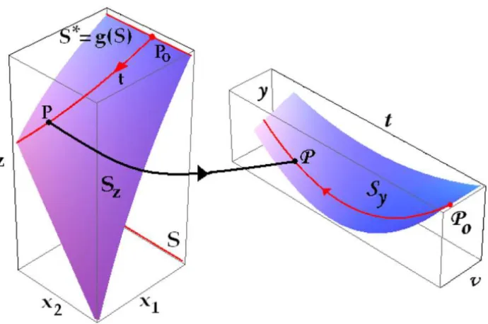
Figure 1 illustrates some of the objects appearing in the proof of Propo-sition 2.1 for n = 2. The label Sz denotes the graph of the unique
solu-tion z(x) to (1) defined on , i.e. Sz = {(x,z(x)),x ∈}. The initial data S∗ def= {(x,z(x)),x ∈S} ⊂ S
z can be described by means of the parametrization
of S as S∗ = {(x,g(x)):x ∈ S}. The left subplot in Figure 1 shows the set
(x1,x2,z(x1,x2)). The initial point P0∈S∗of the curveCx , and a typical point P =(x1,x2,z(x1,x2))∈ Sz, can be observed. On the right, the corresponding
surface solution Sy = {(v,t,y(v,t)):v∈O,t ≥0}, in the(v,t)space is
pre-sented. We show the pointsP,P0 ∈ Sy whereP =(ν,t,y(ν,t))corresponds
toP, i.e. y(ν,t)=z(x,y)).
Concerning the rate of convergence of Picard’s sequences in the first-order PDEs’ context, the following inequality can be advanced for all(v,t)inO0×J:
Yn(v,t)−Y(v,t)
∙ ∙ ∙ =Y0+ Z
0 t
F(Yn−1(v,s))ds−(Y0+ Z
0 t
F(Y(v,s))ds) (13)
≤
Z
0 t
K
Yn−1(v,s)−Y(v,s)
ds≤ K|t|mn−1(v)≤ Kεmn−1(v),
wheremn(v)def= maxt∈J0|Yn(v,t)−Y(v,t)|. Then, by induction
Figure 1 – Surface solution and integral curves.
3 Application to PDEs for boundary values of the Hamilton canonical equations
This section relates first-order PDEs to optimal control problems defined by autonomous, nonlinear systems
˙
x = f(x,u); x(0)=x0∈Rn ; u :[0,T]→Rm ; (15)
coupled to cost functionals of the form
J(T,0,x0,u(∙))= T Z
0
L(x(τ ),u(τ ))dτ+skx(T)k2 , (16)
with smooth LagrangiansLand piecewise continuous admissible control strate-giesu(∙).
The problems will be assumed regular and smooth, i.e. that the value (or Bellman) function
V(t,x),inf
satisfies the Hamilton-Jacobi-Bellman (HJB) equation with boundary condition
∂V
∂t (t,x)+H 0 x, ∂V ∂x ′
(t,x)
=0 (18)
V(T,x)=skxk2 (19)
whereH0is the minimized Hamiltonian defined as
H0(x, λ),H(x, λ,u0(t,x, λ)) , (20) H being the usual Hamiltonian of the problem, namely
H(x, λ,u),L(x,u)+λ′f(x,u) , (21)
andu0is the uniqueH-minimal control satisfying u0
(x, λ),arg min
u H(x, λ,u) , (22)
or equivalently,
H(x, λ,u0(x, λ))≤ H(x, λ,u) ∀u∈U =Rm . (23) Under these conditions, the optimal costate variableλ∗results in
λ∗(t)=
∂V
∂x ′
(t,x∗(t)) , (24)
and the optimal state and costate trajectories are solutions to the Hamiltonian Canonical Equations (HCE)
˙
x =
∂H0 ∂λ
′
,F(x, λ); x(0)=x0, (25)
˙
λ = −
∂H0 ∂x
′
,−G(x, λ); λ(T)=2sx(T), (26)
which in concise form read as one 2n-dimensional ODE
˙
v =X (v) , (27)
v(t), x(t) λ(t)
!
, X (v), F(v)
−G(v) !
with two-point mixed boundary conditions
x(0)=x0, λ(T)=2sx(T) . (29)
When the problem is not completely smooth, i.e. when the resulting value func-tion V is not differentiable, it is still possible to generalize the interpretation of the costate (in Eq. 24) in terms of ‘viscosity’ solutions (see discussion and references quoted in [19], pages 394, 443); but those cases will not be explored here.
The following notation for the missing boundary conditions will be used in what follows:
ρ(T,s) , x∗(T) , (30)
σ (T,s) , λ∗(0) . (31)
The introduction of the variational PDEs is done through the following objects. First of allφ : [0,T] ×Rn×Rn →Rn×Rnwill denote the flow of the Hamil-tonian equations (25-26), i.e.
x(t) λ(t) !
=φ(t,x0, σ )∀t∈ [0,T] ; φ (0,x, λ)= x λ !
, (32)
andφt is thet-advance map defined for eachtas
φt(x, λ),φ (t,x, λ) . (33)
The flow must verify the ODEs of Hamiltonian dynamics, i.e.:
D1φ(t,x, λ)= ∂φ
∂t(t,x, λ)=X(φ t
(x, λ)) . (34)
Let us denote then, for a fixeds,
V(t,s),Dφt(x0, σ (T,s)) . (35)
It can be shown, by deriving ODE condition in Eq. (34) with respect to the
(x, λ)-variables, that the following ‘variational (ODE) equation’ (see [14]) applies:
˙
where
A(t,s), DX◦φt(x0, σ (T,s))=DX(ρ(T,s),2sρ(T,s)) , (37)
and V˙(t,s) stands for ∂V∂t(t,s). Now it should be noted that V(t,s) is the fundamental matrix8(t,0)of the linear system
˙
y =A(t,s)∙y, (38)
i.e. its solution is y(t) = 8(t, τ )y(τ ), 8(τ, τ ) = I, and it can be shown (see [19]) that the matrixV(T,s)=8(T,0)verifies
VT =A(T,s)V , V(0,s)=I , (39)
a first-order PDE which, given the form of Eq. (37), must be solved together with a pair of equations forρ(T,s), σ (T,s). It turns out that several equivalent equations may play this role, for instance [6]
V′
1(2sρT +G)+V3′(F−ρT)=σT (40) V′
1(2ρ+2sρs)−V3′ρs =σs (41)
where theVi,i=1, . . .4 are the partitions inton×nsubmatrices of
V = V1 V2 V3 V4 !
,
and
F(ρ,s),F(ρ,2sρ), G(ρ,s),G(ρ,2sρ) . (42)
In the one-dimensional case Eqs. (39, 40, 41) can be replaced [5] by
ρρT −
s F(ρ,s)+G(ρ,s)
2
ρs =ρF(ρ,s), ρ(0,s)=x0 (43)
ρσT −
s F(ρ,s)+G(ρ,s)
2
σs =0, σ (0,s)=2sx0. (44) It is possible first to calculate ρ(T,s) by solving Eq. (43), and afterwards
Now, the iterative method proposed in Section 2 will be applied to solve Eq. (43). The Picard scheme uses an arbitrary guess ρ0(T,s) for the solution and attempts to solve
ρT − s F
(ρ0,s) ρ0 +
G(ρ0,s)
2ρ0
ρs =F(ρ0,s) , (45)
where only the variableρ is replaced byρ0(T,s)the derivatives of ρ
remain-ing unknown. It is enough to search for the integral curves of the vector field
C(T,s)=(1, Ŵ(ρ0,s),F(ρ0,s)), where
Ŵ(ρ0,s),− s F
(ρ0,s) ρ0 +
G(ρ0,s)
2ρ0
, (46)
i.e. to solve the system of ODEs
dT dt =1,
ds
dt =Ŵ(ρ0,s) , dy
dt =F(ρ0,s). (47)
The first equation impliesT =t, then
ds
dt =Ŵ(ρ0(t,s),s) , s(0)=s0 (48)
can be solved alone, to finds(t,s0), and finally the ODE forytakes the form dy
dt = F(ρ0(t,s(t,s0)),s(t,s0)) , y(0)=x0. (49)
A grid (Ti,sk) can be constructed on the (T,s) space but with s(Ti) = sk.
Afterwards Eq. (49) can be numerically solved and the value y(Ti,s(Ti)) is
picked up. According to (6)
ρ(Ti,sk)= y(Ti,s(Ti)) . (50)
Finally an interpolation is made to obtain an approximation of ρ(T,s). The result of this interpolation is ρ1, and so on. Were the calculations exact, the constructed sequence of functions{ρn}should then converge toρ.
4 Numerical examples
Three examples are treated in this section. One of them is just an abstract PDE whose analytical solution is known. The remaining examples come from optimal control problems (regularity and smoothness properties hold, as can be checked in the references quoted for each case).
4.1 Case-study 1: a one-dimensional nonlinear control system with a quad-ratic cost
The results of the previous sections will be applied here to the following initial-ized dynamics
˙
x = −x3
+u ; x(0)=x0=1, (51)
subject to the quadratic optimality criterion
J(u)= T Z
0
x(t)2+u2(t)
dt+Sx(T)2. (52)
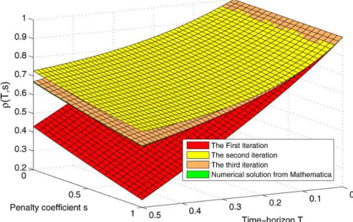
The problem presented in this subsection has been treated in [18] as a hyper-sensitive boundary value problem (HSBP), since small perturbations seriously affect its numerical solution for long time-horizonsT. The corresponding vari-ational PDEs were posed in [11] and they were solved numerically by using the
MATHEMATICAr software package (specifically, the command “NDSolve”) andMATLABr(using the command “pdepe”). For the regulation case they read as follows
ρT =(−4sρ2−s2+1) ρs−(ρ3+sρ); ρ(0,s)=1 (53)
σT =(−4sρ2−s2+1) σs; σ (0,s)=2sx0=2s (54)
Figure 2 – Picard scheme applied to a one-dimensional case for which standard software is acceptable.
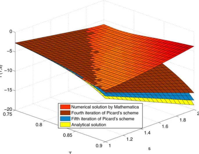
4.2 Case-study 2: a one-dimensional PDE with analytical solution
This is an example that can be solved analytically. The PDE and its initial condition are the following:
rt +rs(s(t−1)+r−1)= −2s, r(0,s)=1∀s ,
whose exact solution reads
r(t,s)=1+s
1−t− 1 1−t
.
Figure 3 – Several Picard iterations converging to the analytical solution (yellow)vs. numerical solution using the command “NDSolve”.
system (3-4) takes the form
∂T
∂t (v0,t) = 1, T(v0,0)=0 ∂s
∂t(v0,t) = s(T −1)+r −1, s(v0,0)=v0 (55) ∂r
∂t(v0,t) = −2s, r(v0,0)=1
and, in the notation of Section 2
Y(t)=(T(t),s(t),r(t)),
F(Y(t))= F(T(t),s(t),r(t))=(1,s(T −1)+r −1,−2s),
ForT ∈ [0,1], v ∈ [1,2],r ∈ [0,1], the Lipschitz constant can be chosen as the upper bound for the derivative. The valuesK =√10,M =√26, are found admissible, and therefore
|yn(v,t)−y(v,t)| ≤mn(v)≤(
√
10ε)n.
From the exact solutionY(v,t)=(t, v(1−t),1−v+v(1−t)2)and using
ε < 1/√26 < 1/√10, the analytical expressions of the iterations allow to check, for increasingn,
Y1(v,t) = (t, v(1−t),1−2vt), |Y1−Y| =v2t2<4ε2≪
√
10ε;
Y2(v,t) = (t, v(1−t)−vt3/3,1−2vt+vt2),
|Y2−Y| = vt3/3<2ε3/3≪ √
10ε 2
;
Y3(v,t) = (t, v(1−t)−vt5/15−vt4/12, (1−vt)2+vt4/6),
|Y3−Y| = vt4/6<2ε4/6≪ √
10ε 3
.
4.3 Case-study 3: a two-dimensional nonlinear control system with a quad-ratic cost
The well-known time-variant Linear-Quadratic-Regulator (LQR) problem is here revisited (see [12] for related results). Such a problem is defined by
˙
x = −x +e−tu
, f(t,x,u) , (56)
L(t,x,u)=u2, A(t)≡ −1, B(t)=e−t, (57)
Q(t)≡0, R(t)≡1, S=s I,s ≥0, (58)
K(x)=s[x(T)]2 . (59) The problem is transformed into an autonomous one through the usual change of variables
x →x1, t →x2 , (60)
and for simplicity the old symbolx will be maintained for the new state, i.e., in what follows,
and, in the new set-up the (autonomous) dynamics will read
˙
x = fa(x,u),(f(t,x1,u),1)′,
˙
x1= −x1+e−x2u, x1(0)=x0, (62)
˙
x2=1, x2(0)=0. (63)
The transformed cost functional, Lagrangian, and final penalty will then be
Ja(T,0, (x0,0)′,u(∙)), T Z
0
La(x(τ ),u(τ ))dτ +Ka(x) , (64)
La(x,u),u2=L(t,x1,u) , (65) Ka(x),sx12=diag(s,0)x = K(x1) . (66)
It is clear that the optimal control for both (the time-variant and the auto-nomous) problems will be the same, since
Ja(T,0, (x0,0)′,u(∙))=J(T,0,x0,u(∙)) , (67) however the new dynamics is nonlinear (actually, Eq. (62) having an exponen-tial, implies that all powers of x1 are present, and they are multiplied by the
control). New expressions for the Hamiltonian Ha, the H-minimal controlu0a,
and the minimized (or control) HamiltonianH0
a will apply, namely
Ha(x, λ,u) , La(x,u)+λ′fa(x,u) (68)
= Ru2+λ1(−x1+e−x2u)+λ2, (69) u0
a(x, λ),arg minu H(x, λ,u)= −
1 2Re
−x2λ1, (70)
H0
a(x, λ), Ha(x, λ,u0(x, λ))= −x1λ1−
1 4Re
−2x2λ2
1+λ2, (71)
and the HCE for this case will read in component-by-component form
˙
x1 = −x1−
1 2e
−2x2λ1, x1(0)=x
0, (72)
˙
x2 = 1, x2(0)=t0=0, (73)
˙
λ1 = λ1, λ1(T)=2sx1(T) , (74)
˙
λ2 = −
1 2e
−2x2λ2
This ODEs can be solved analytically, to obtain
x1(t) = e−t
x0− t
2c1
, (76)
x2(t) = t−t0=t, (77) λ1(t) = c1et ,c1=
2s
e2T +sT , (78) λ2(t) = c3−
1 2c
2
1t, c3= T
2c
2
1. (79)
X(x, λ) =
−x1−12e−2x2λ1
1
λ1
−12e− 2x2λ2
1 (80)
DX(x, λ) = A(t,s)=
−1 c1e−t −12e−2t 0
0 0 0 0
0 0 1 0
0 c12 −c1e−t 0 . (81)
Then, the linear time-variant variational equation (36) can also be integrated analytically, and its solution results
V(t,s) =
e−t c
1te−t −12te−t 0
0 1 0 0
0 0 et 0
0 c2
1t −c1t 1 . (82)
The PDEs (39)-(41) were solved numerically by usingMATHEMATICAr, and their solutions compared against the following analytical expressions
V(T,s) =
e−T 2sT e−T
e2T+sT −12T e− T 0
0 1 0 0
0 0 eT 0
0 4s2T
(e2T+sT)2 −
2sT e2T+sT 1
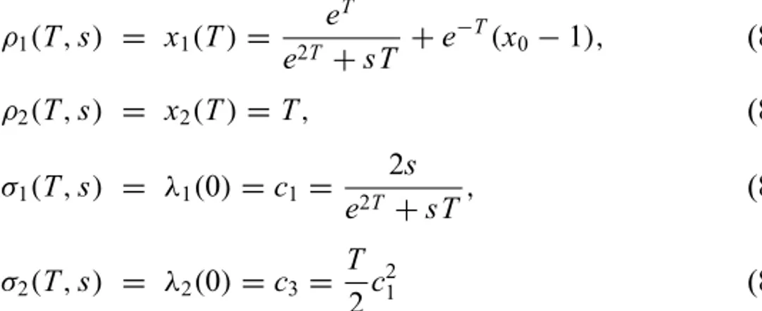
ρ1(T,s) = x1(T)= e T
e2T +sT +e− T
(x0−1), (84) ρ2(T,s) = x2(T)=T, (85) σ1(T,s) = λ1(0)=c1=
2s
e2T +sT, (86) σ2(T,s) = λ2(0)=c3=
T
2c
2
1 (87)
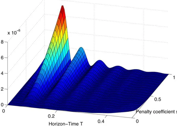
In Figure 4 the results of applying the new method to Eq. (39-41) are illustrated. The relative error of the seventh Picard iteration with respect to the analytical solution is shown in Figure 5. It is of the same order than the one reached through standard software calculations.
Figure 4 – Picard scheme applied to the two-dimensional (nonlinear) version of the time-variant LQR problem, for which standard software’s solution is acceptable.
5 Conclusions
Figure 5 – Relative error between the seventh Picard iteration and the analytical solu-tion to the LQR.
no systematic comparisons against specialized numerical approaches (like ad-vanced finite differences and finite elements schemes) have been attempted in the paper, at least the method proposed here has worked better than standard mathematical software likeMATHEMATICArandMATLABrin all cases.
The fact that the Picard’s method always converge in the ODE context (assum-ing the existence of a unique solution and precise calculations at each iteration step) was used to prove convergence of the scheme for the PDEs under study. The solution surfaces corresponding to each Picard step uniformly converge to the solution surface to the original PDE. This convergence guarantees that the accuracy of results can be improved with respect to non-iterative methods (like finite differences in their different versions). Analytical bounds for the rate of convergence have been found, and checked in a case-study whose explicit solu-tion is known.
optimal control problem for nonlinear systems have been solved numerically in a satisfactory way by the new method. This application is particularly use-ful given the hyper-sensitivity of Hamilton Canonical Equations (HCEs), whose boundary values are obtained from the variational PDEs’ solutions, and there-fore need to be highly accurate.
REFERENCES
[1] A. Abdelrazec and D. Pelinovsky, Convergence of the Adomian decomposition method for initial-value problems. Numerical Methods for Partial Differential Equations, (2009), DOI 10.1002/num.20549.
[2] R. Bellman and R. Kalaba, A note on Hamilton’s equations and invariant imbed-ding. Quarterly of Applied Mathematics,XXI(1963), 166–168.
[3] P. Bernhard, Introducción a la Teoría de Control Óptimo, Cuaderno Nro. 4, Instituto de Matemática “Beppo Levi”, Rosario, Argentina (1972).
[4] V. Costanza, Optimal two Degrees of Freedom Control of Nonlinear systems. Latin American Applied Research, (2012), to appear.
[5] V. Costanza,Finding initial costates in finite-horizon nonlinear-quadratic optimal control problems. Optimal Control Applicantions & Methods, 29(2008), 225– 242.
[6] V. Costanza, Regular Optimal Control Problems with Quadratic Final Penalties. Revista de la Unión Matemática Argentina,49(1) (2008), 43–56.
[7] V. Costanza, R.A. Spies and P.S. Rivadeneira, Equations for the Missing Bound-ary Conditions in the Hamiltonian Formulation of Optimal Control Problems. Journal of Optimization Theory and Applications,149(2011), 26–46.
[8] V. Costanza and C.E. Neuman, Partial Differential Equations for Missing Bound-ary Conditions in the Linear-Quadratic Optimal Control Problem. Latin American Applied Research,39(2008), 207–211.
[9] V. Costanza and P.S. Rivadeneira, Hamiltonian Two-Degrees-of-Freedom Control of Chemical Reactors. Optimal Control Applicantions & Methods, 32(2011), 350–368.
[11] V. Costanza and P.S. Rivadeneira,Finite-horizon dynamic optimization of nonlin-ear systems in real time. Automatica,44(9) (2008), 2427–2434.
[12] V. Costanza and P.S. Rivadeneira,Initial values for Riccati ODEs from variational PDEs. Computational and Applied Mathematics,30(2011), 331–347.
[13] G.B. Folland, Introduction to Partial Differential Equations. Second Edition. Princeton University Press (1995).
[14] M. Hirsch and S. Smale, Differential Equations, Dynamical Systems and Linear Algebra. Academic Press, New York (1974).
[15] R. Murray,Optimization Based-Control. California Institute of Technology, Cal-ifornia, in press (2009).
http://www.cds.caltech.edu/∼murray/amwiki/Supplement:_Optimization-Based_Control
[16] G.E. Parker and J.S. Sochacki, A Picard-Maclaurin theorem for initial value PDEs. Abstract and Applied Analysis,5(1) (2000), 47–63.
[17] G.E. Parker and J.S. Sochacki,Implementing the Picard iteration. Neural, Parallel and Scientific Computations,4(1) (1996), 97–112.
[18] A.V. Rao and K.D. Mease,Eigenvector approximate dichotomic basis method for solving hyper-sensitive optimal control problems. Optimal Control Applications & Methods,21(2000), 1–19.
[19] E.D. Sontag,Mathematical Control Theory. Springer, New York (1998). [20] A.I. Zenchukand and P.M. Santini, Dressing method based on homogeneous