ISSN 0101-8205 / ISSN 1807-0302 (Online) www.scielo.br/cam
A stabilized finite element method to pseudoplastic
flow governed by the Sisko relation
MARCIO ANTÔNIO BORTOLOTI1 and JOSÉ KARAM FILHO2∗ 1Departamento de Ciências Exatas, Universidade Estadual do Sudoeste da Bahia, UESB,
Estrada do Bem-Querer, Km 4, 45083-900 Vitória da Conquista, BA, Brazil 2Coordenação de Mecânica Computacional, Laboratório Nacional de Computação Científica,
LNCC, Av. Getúlio Vargas, 333, 25651-070 Petrópolis, RJ, Brazil E-mails: [email protected] / [email protected]
Abstract. In this work, a consistent stabilized mixed finite element formulation for incom-pressible pseudoplastic fluid flows governed by the Sisko constitutive equation is mathematically analysed. This formulation is constructed by adding least-squares of the governing equations and of the incompressibility constraint, with discontinuous pressure approximations, allowing the use of same order interpolations for the velocity and the pressure. Numerical results are presented to confirm the mathematical stability analysis.
Mathematical subject classification: Primary: 65M60; Secondary: 65N30.
Key words:finite element method, numerical analysis, Sisko relation, non-Newtonian flow.
1 Introduction
In modeling some kinds of fluids, the Sisko constitutive relation comes out from the Cross model [6], when the apparent viscosity lies in a range between the pseudoplastic region and the lower Newtonian plateau. A good alterna-tive constitualterna-tive equation of the Sisko type for blood flow has been proposed by [13], for example.
The nonlinearity of this relation together with the incompressibility constraint may generate numerical instabilities when some classical numerical methods are used. For classical methods, in case of velocity and pressure formulations, it is well known that, even for the linear case, different interpolation orders for these variables have to be used in order to satisfy the Babuška-Brezzi stability condition [2, 4].
In this work, to avoid the use of penalization methods or reduced integration and to recover the stability and accuracy of the solution of same interpolation orders in primitive variables, a consistent mixed stabilized finite element formu-lation is presented. It is constructed by adding the least-squares of the governing equations and the incompressibility constraint, with continuous velocity and discontinuous pressure interpolations. The present formulation is here mathem-atically analysed based on Scheurer’s theorem, [12]. Stability conditions and error estimates are established when the Sisko relation is considered. Numerical examples are presented to confirm the stability analysis.
2 Definition of the problem
Let be a bounded domain in Rn where the positive integer n, denotes the
space dimension. We consider the stationary incompressible creep flow problem governed by−divσ = f in, where σ : → Rn
×Rn denotes the Cauchy
stress tensor for the fluid andf denotes the body forces.
The governing equation, written above, is subjected to the incompressibility constraint divu=0 in, whereudenotes the velocity field.
The Sisko model is characterized by a linear supersposition between the Newtonian and the pseudoplastic effects, presenting a dependence of the viscos-ityμwith the shear-strain rate tensor, defining an apparent viscosityμ(|ε(u)|), leading to the stress tensor of the form
σ = −pI+μ(|ε(u)|)ε(u) with μ(|ε(u)|)=λ1+λ2ν(|ε(u)|) andν(s)=sα−2, whereλ
1, λ2are two positive constitutive constants,α ∈ ]1,2[ is the power index, p is the hydrostatic pressure,I ∈ Rn
×Rn is the identity
tensor,| ∙ |denotes the Euclidean tensor norm and ε(u)= 1
2
is the symmetric part of the gradient ofu.
With the above considerations, together with boundary condition of Dirichlet type, the resulting problem is: find(u,p)∈C2()×C1()such that
−div(μ(|ε(u)|)ε(u))+ ∇p = f in divu = 0 in
u = uon∂
(1)
where∂denotes the boundary of.
Physically, pseudoplastic flows are characterized by a viscosity decreasing continuously and smoothly with increasing of shear rate, and this behaviour occurs in a limited range of shear rate, generating the viscosity plateaus, where we can see that the apparent viscosityμ(s) is a bounded continuous function such that
μ∞≤μ(s)≤μ0 (2)
for 0 < g0 ≤ s ≤ g∞ with g0 and g∞ being the shear rate finite limits and μ0andμ∞corresponding to the finite limiting Newtonian plateaus for low and high shear rate, respectively, [3].
It can be seen that from continuous classical Galerkin formulation associated with problem (1), we can obtain
kε(u)k0 ≤
C
μ∞kfk0 (3)
for allu∈W01,2(), whereC is the constant in Poincaré’s inequality.
3 Petrov-Galerkin-Like formulation
To generate the stabilized finite element method proposed here, the following definitions will be used.
Let Lp()
= {u|uis measurable, R|u(x)|pd <
∞} be the class of all
measurable functionsu, such that,uis p-integrable inand letL0p()= {u∈ Lp(), R
u d =0}be the class of functions in L
p()such thatu has null
mean. Let Wm,p() be the Sobolev space Wm,p() = {u ∈ Lp()|Dβu ∈ Lp(),0
≤ |β| ≤m}with
Dβu= ∂
whereβi is a natural integer and|β| =β1+ ∙ ∙ ∙ +βm. TheW m,p
0 ()is defined as the space of functionsu∈Wm,p()such thatDβu
=0 on∂, for allβwith
|β| ≤m−1, [1].
The norm in the spaceWm,p()is defined as
kukm,p=
X
|β|≤m
kDβukp
1/p
, 1≤ p<∞,
wherekukpis theLp()norm defined as
kukp= Z
|u(x)|pd x 1/p
, x ∈.
In this paper, we will denotekuk1= kuk1,2andkuk0 = kuk2.
We assume for simplicity ⊂ Rn, a polygonal domain discretized by a classical uniform mesh of finite elements with Neelements, such that
=
Ne
[
e=1
e, ei
∩ej
= ∅ for all i 6= j
wheree denotes the interior of the et helement andeis its closure.
Let Shk() be the finite element space of the Lagrangean continuous poly-nomials inof degreekandQlh()the finite element space of the Lagrangean discontinuous polynomials inof degreel. Thus we can define the
approxima-tion spacesVh =(Shk()∩W
1,2
0 ())n andWh = Qlh()∩L2()to velocity
and pressure respectively, that can be generated by triangles or quadrilaterals.
Remark 3.1. For the Galerkin method,kandlmust be different orders even for k ≥ 2 and one can follow [7, 8] and [9], for example, to see the limitations for
the combinations ofkandl.
Remark 3.2. With the present consistent stabilized formulation, all the
combi-nations of different orders are possible, optimal and suboptimal, but it is possible to use same orders fork andl, with complete polynomials, providingk ≥2, as
follows.
of the linear momentum and of the continuity equations to the Galekin formula-tion, generating the following problem with homogeneous boundary condition considered without lost of generalities:
Problem PGhd. Givenf ∈W−1,2(), the dual ofW1,2(), findUh ∈Vh×Wh, such that
(Ah(Uh),Vh)+Bh(ph,vh)=Fh(Vh) ∀ Vh∈Vh×Wh
Bh(qh,uh)=0 ∀ qh ∈Wh where
(Ah(Uh),Vh)=(μ(|ǫ(uh)|)ε(uh), ε(vh))+δ2ϑ (divuh,divvh)
+δ1h
2
ϑ (−1μuh+ ∇ph,−1μvh+ ∇qh)h,
(4)
Bh(ph,vh)= −(ph,divvh), (5)
Fh(Vh)=f(vh)+δ1h
2
ϑ (f,−1μvh+ ∇qh)h, (6) withhdenoting the mesh parameter,μ(|ε(uh)|)the apparent viscosity,
(u, v)=
Z
uvd x, (u, v)h= Ne
X
e=1
Z
e
uvd x,
δ1 and δ2 being positive constants denoted as stability parameters, 1μuh = div(μ(|ε(uh)|)ε(uh)),Uh = {uh,ph},Vh= {vh,qh}andϑbeing a dimensional
parameter. We can note that when δ1 = δ2 = 0, Problem PGhd reduces to
the Galerkin formulation which, for interpolations of same order, is unstable exhibiting spurious pressure modes or presenting the locking of the velocity field, [9]. The nonlinear Problem PGhd preserves the good properties of the
linear analogous of [11] in the sense that it accommodates, for k ≥ 2
equal-order interpolations for velocity and pressure as will be shown in the following analysis and confirmed later by the obtained numerical results.
4 Finite element analysis
The finite element analysis is developed here by considering solutions in Hilbert Spaces, as in [10]. We start the analysis by rewriting the discontinuous pres-sure approximationphas
ph = ph∗+ ph, (7)
with p∗
h ∈ W∗h and ph ∈ Wh where W∗h = {p∗h ∈ Wh ∩ L20(e),∇peh = ∇ph}∗ is the subspace of the pressure with zero mean at the element level and Wh = {ph ∈ Wh; ∇peh = 0,p
e h =
R
e pehde/
R
ede}is the subspace of the piecewise constant pressure, where phe represents the constraint of ph in
elemente.
The discontinuous pressure allows the satisfaction of the incompressibility constraint at element level in contrast to the continuous approximations, which satisfies the constraint only in global sense. Considering this segregation, the Problem PGhdcan be rewritten as the following variational form, which
consid-ers the pressure variablephwritten as functions of p∗
h ∈W∗h()and ph ∈Wh,
as was described above:
Problem PG∗
hd. Given f ∈ W−
1,2(), find
{uh,p∗
h,ph} ∈ Vh×W∗h×Wh, such that
(A∗
h(Uh∗),Vh∗)+Bh(ph,vh)= Fh∗(Vh∗) ∀ Vh∗∈Vh×W∗h
Bh(qh,uh)=0 ∀ qh∈Wh where
(A∗h(Uh∗),Vh∗)=(μ(|ε(uh)|)ε(uh), ε(vh))+Bh(p∗h,vh)+Bh(qh∗,uh)
+δ2ϑ(divuh,divvh)+δ1h 2
ϑ (−1μuh+ ∇p ∗
h,−1μvh+ ∇qh∗)h,
(8)
Bh(p∗h,vh)= −(ph∗,divvh), (9) Bh(ph,vh)= −(ph,divvh), (10) Fh∗(Vh∗)=f(vh)+δ1h
2
ϑ (f,−1μvh+ ∇q ∗
h)h, (11)
U∗
Lemma 4.1. Forμ(s)bounded, continuous and smooth real function such that |dμ(s)/ds| ≤M, there exists a positive constant C, independent of h, such that hk1μuhk0h≤Ckε(uh)k0wherekuk20h =(u,u)h.
Proof. From the inverse estimate
hkdivε(uh)k0h≤Chkε(uh)k0, (12) typical of finite element methods, [5], 0 < μ∞ ≤ μ(s) ≤ μ0 and|dμ(s)/ds|
≤ M, we have the inverse estimate proposed, withC =μ0Ch+M.
Lemma 4.2. Assuming the same considerations of Lemma 4.1, there is a positive constant Cl, independent of h, such that, hk −1μuh +1μvhk0h ≤ Clkε(uh)−ε(vh)k0for alluh,vh ∈Vhwith h>0.
Proof. From the triangular inequality, the Lemma 4.1 and (12) we have h2k −1μuh+1μvhk20h ≤4[(μ
2
0Ch2+M
2)
kε(uh−vh)k20
+(1+Ch2)kε(vh)k02kμ(uh)−μ(vh)k20h]. The mean value theorem yields
h2k −1μuh+1μvhk20h≤4
(μ20Ch2+M
2
)kε(uh)−ε(vh)k20
+(1+Ch2)kε(vh)k20 sup 0≤θ≤1 k∇
μ(|ε((1−θ )uh+θvh)|)k20hkuh−vhk20h
.
Since |dμ(s)/ds| ≤ M for all uh ∈ Vh and from Korn’s inequality, we can conclude the result, with the constantCl given by
Cl =4 "
(μ20Ch2+M2)+(1+Ch2)M2C2K sup
vh∈Vh k ε(vh)k20
#
whereCK is the constant of the Korn’s inequality. The lemma is obtained as a
consequence of
kε(uh)k0≤C(λ1, λ2, μ∞,C, δ1, )kfk0 for all uh ∈Vh, (13)
that is, naturally, obtained from Problem PGhd and consequently yieldsCl as a
Definition 4.3. Letk|Uh|k = kUhk +h(kdivε(uh)k0h+ kε(uh)k0h+ k∇phk0h) be a mesh-dependent norm on the product space H01()× L2(), where h denotes the mesh parameter andkUhk2= kuhk21+ kphk20is the norm defined in
Vh×Wh.
Lemma 4.4 (Equivalence of the norms). There exists a positive constantκ
such thatkUhk ≤ k|Uh|k ≤κkUhkfor all Uh∈Vh.
Proof. The inequalitykUhk ≤ k|Uh|kis immediate. In other hand, from the
definition ofk|Uh|k, from the inverse estimate (12) and from the inverse estimate
for the pressure, see [5],
hk∇p∗hk0h≤Cpkp∗hk0,
we havek|Uh|k ≤ kUhk +(Ch+1)kε(uh)k0+Cpkphk0. Using the classical inequality,
1
√
nkdivuk0≤ kε(u)k0≤ kuk1, (14)
we complete the proof of Lemma 4.4, withκ =1+max{Ch+1,Cp}.
With the above results we can establish the following result that will be needed later to generate the estimates in Theorem 4.9.
Theorem 4.5.There exists a positive constantγcsuch that
|(A∗h(U∗)−Ah∗(Vh),Uh∗−Vh∗)| ≤γck|U∗−Vh∗|k kUh∗−Vh∗k
for all U∗∈W01,2()×L2()and Uh∗,Vh∗ ∈Vh×W∗h.
Proof. By the consistency of the problem PG∗hdand from (4) we have |(A∗h(U∗)−A∗(Vh∗),Uh∗−Vh∗)| ≤λ1|(ε(u−vh), ε(uh−vh))|
+λ2|(ν(|ε(u)|)ε(u)−ν(|ε(vh)|)ε(vh), ε(uh−vh))| + |Bh(ph∗−qh∗,u−vh)| +δ2ϑ|(divu−divvh,divuh−divvh)| + |Bh(p∗−qh∗,uh−vh)|
+δ1h
2 ϑ
−1μu+1μvh+ ∇(p
∗
−qh∗),−1μuh+1μvh+ ∇(ph∗−qh∗)
From the continuity of the two first terms in the right hand side above, [12], and using the inequality (14) we have
|(A∗h(U∗)− A∗h(Vh∗),Uh∗−Vh∗)| ≤ [(λ1+λ2+nϑ δ2)ku−vhk1
+√nkp∗−qh∗k0]kuh−vhk1+δ1
h
ϑ
× kν(|ε(u)|)divε(u)−ν(|ε(vh)|)divε(vh)k0h + k∇p∗− ∇qh∗k0h+ kε(u)∇μ(u)−ε(vh)∇μ(vh)k0h
× kuh−vhk1+ kp∗h−qh∗k0
.
By using Lemma 4.2 and identifying thek| ∙ |knorm, we can conclude
|(A∗h(U∗)−Ah∗(Vh∗),Uh∗−Vh∗)| ≤γck|U∗−Vh∗|k kUh∗−Vh∗k,
whereγc=max{λ1+λ2+nϑ δ2,√n,δϑ1}.
Theorem 4.6. Let Kh = {vh ∈ Vh,Bh(qh,vh) = 0, for all qh ∈ Wh}. Then,
there exists a positive constantγe such that(A∗h(Uh∗)− A∗h(Vh∗),Uh∗−Vh∗) ≥
γekUh∗−Vh∗k
2for all U∗
h,Vh∗∈ Kh×Wh∗. Proof. From (8) we obtain
(A∗h(Uh∗)−A∗h(Vh∗),Uh∗−Vh∗)≥λ1kε(uh−vh)k20
+δ2ϑkdivuh−divvhk20h+2Bh(p∗h−qh∗,uh−vh)
+δ1h
2
ϑ k −1μuh+1μvh+ ∇(p ∗
h−qh∗)k
2 0h +λ2 ν(|ε(uh)|)ε(uh)−ν(|ε(vh)|)ε(vh), ε(uh−vh)
.
From the ellipticity of the last term in the right hand side above, presented in [12], and using the Young inequality withξ = δ1
2ϑ we have
(A∗h(Uh∗)−A∗h(Vh∗),Uh∗−Vh∗)≥(γ λ2+λ1)kε(uh)−ε(vh)k
2 0
+δ1h
2
ϑ k1μuh+1μvh+ ∇(p ∗
h−qh∗)k
2 0h−
1 δ2ϑk
Applying again the Young inequality it yields
(A∗h(Uh∗)−A∗h(Vh∗),Uh∗−Vh∗)≥(γ λ2+λ1)kε(uh)−ε(vh)k20
−δ1
2ϑk
ph∗−qhk∗ 20+δ1h
2 ϑ (1−
1
η)k −1μuh+1μvhk 2 0h
+δ1h
2
ϑ (1−η)k∇p ∗
h− ∇qh∗k
2 0h,
withη > 0. From Lemma 4.2 and consideringr1andr2 as two positive con-stants, such that 1
r1 + 1
r2 =1, we can rewrite the previous inequality as (A∗h(Uh∗)−A∗h(Vh∗),Uh∗−Vh∗)≥ γ λ2+λ1
r1 k
ε(uh)−ε(vh)k20
+h2
γ λ2+λ1
r2Cl + δ1 ϑ
1− 1 η
k −1μuh+1μvhk20h
+δ1h
2
ϑ (1−η)k∇p ∗
h−qh∗k
2 0h−
1 δ2ϑkp
∗
h−qh∗k
2 0. Choosingη= δ1r2Cl
(γ λ2+λ1)ϑ+δ1r2Cl), we obtain
(A∗h(Uh∗)−A∗h(Vh∗),Uh∗−Vh∗)≥ γ λ2+λ1
r1 kε(uh)−ε(vh)k 2 0
− 1
δ2ϑk
p∗h−qh∗k20+ δ1(γ λ2+λ1)h
2
ϑ (γ λ2+λ1)+δ1r2Cl)k∇(
ph∗−qh∗)k20h.
By using the inequality
h2k∇qh∗k20h≥ kqhk∗ 20, (15) as in [10], and the Korn’s inequality, we have
(A∗h(Uh∗)−A∗h(Vh∗),Uh∗−Vh∗)≥γe(kuh−vhk21+ kph∗−qh∗k
2 0) with
γe =min
(γ λ2+λ1)C
r1 ,
δ1(γ λ2+λ1) ϑ (γ λ2+λ1)+δ1r2Cl −
1 δ2ϑ
,
since
δ1(γ λ2+λ1) ϑ(γ λ2+λ1)+δ1r2Cl −
1 δ2ϑ
>0. (16)
The inequality (16) gives a sufficient condition, providing a useful relation to be used to choose the stabilizing parameters.
Theorem 4.7. There exists a positive constantγB such that
Bh(p− ph,uh−vh)≤γBkp−phk0kUh∗−Vh∗k for all p∈ L2(),U∗
h,Vh∗∈Vh×W∗h.
Proof. This result comes from the application of the Hölder-Schwarz
inequal-ity and by the use of (14).
Theorem 4.8. For k ≥ 2 and since Vh ∈ Vh ×Wh, there exists a positive
constantβh, independent of h, such that
sup vh∈Vh
|Bh(qh,vh)|
kvhk1 ≥βhkqhk0 for all qh∈Wh.
Proof. This result may be seen in [7].
With the above results, we can establish the following error approximation estimates.
Theorem 4.9. There exists a positive constantζh, independent of h, such that the following estimate holdsk|U −Uh|k ≤ζhk|U−Vh|k.
Proof. From the definition of(A∗h(∙),∙)and the consistency of the formula-tion we can write
A∗h(Uh∗)−A∗h(Vh∗),Uh∗−Vh∗= A∗h(U∗)−A∗h(Vh∗),Uh∗−Vh∗
+ A∗h(Uh∗)−Ah∗(U∗),Uh∗−Vh∗
(17)
with
A∗h(Uh∗)−A∗h(U∗),Uh∗−Vh∗
= Bh p−qh,uh−vh
. (18)
Replacing (18) in (17) we have
A∗h(Uh∗)−A∗h(Vh∗),Uh∗−Vh∗= A∗h(U∗)−A∗h(Vh∗),Uh∗−Vh∗ +Bh p−qh,Uh∗−Vh∗
From Theorem 4.5, Theorem 4.6, Theorem 4.7 and considering the norm equiv-alence betweenk| ∙ |kandk ∙ kestablished in Lemma 4.4, we have
k|U∗−Uh∗|k ≤
1+γc γe
k|U∗−Vh∗|k +
γB
γek
p−qhk0. (19) In order to obtain an estimate tokp− phk0, we note that from PGhd problem,
we have
Bh ph,uh−vh
= A∗h(U∗)−A∗h(Uh∗),Uh∗−Vh∗+Bh p,uh−vh
.
Sincevh ∈ Kh, then
Bh ph−qh,uh−vh
= A∗h(U∗)−A∗h(Uh∗),Uh∗−Vh∗
+Bh p−qh,uh−vh
.
Using Theorem 4.5 and Theorem 4.7 we have sup
wh∈V∗h
Bh(ph−qh,wh)
kwhk1+ kp∗h−qh∗k0
≤ k|U∗−Vh∗|k + kp−qhk0. By the use of Theorem 4.8, we can see that
kp−phk0≤ 1 βhk
U∗−Vh∗kh+
1+ 1 βh
kp−qhk0. (20) Combining (19) and (20) we have
k|U∗−Uh∗|k ≤ζhk|U∗−Vh∗|k,
where
ζh=1+
1 βh +
1 γe
max
γc, γB ,
sincekphk20= kph∗k20+ kphk20. From Theorem 4.9, applying inverse estimates and the very classical interpo-lation results presented in, for example, Chapter 3 of [5], we obtain the following error estimate
kU−Uhk ≤ζh(2+Ch)c1hk|u|k+1+ζh(1+Cp)c2hl+1|p|l+1 (21) withc1,c2 ∈ R, uh ∈ Shk()and ph ∈ Q
l
5 Numerical results
In order to obtain numerical results for the finite element method presented here to nonlinear problem, the following numerical algorithm will be used. There are many methods to solve nonlinear equations. In this case, we lag nonlinear terms in the system of equations and start with an initial guess generating a sequence of functions that is expected to converge for the solution. In this sense, our scheme is constructed by: givenuh0∈Vh, lets find(uhn,p
n
h)∈Vh×Wh,n=1,2,3, . . . such that
(μ(|ε(unh)|)ε(unh+1), ε(vh))+Bh(phn+1,vh)+Bh(qh,u
n+1 h )
+δ1h
2
ϑ (−div(μ(u n h)ε(u
n+1
h ))+ ∇p∗
n+1
h ,−1μvh+ ∇qh)h
+δ2ϑ(divuhn+1,divvh)= Fh∗(Vh∗),∀Vh ∈Vh×Wh.
0 0.2 0.4 0.6 0.8 1
-0.4 -0.2 0 0.2 0.4 0.6 0.8 1
y
Horizontal Velocity
λ1 =0.1, λ2 = 1.0, α = 1.3 λ1 =1.0, λ2 = 0.1, α = 1.3 λ1 =1.0, λ2 = 1.0, α = 1.3 Newtonian Flow
Figure 1 – Horizontal velocity atx=0.5
(a) Velocity field (b) Pressure field
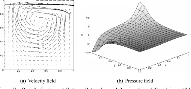
Figure 2 – Results forλ1=1.0,λ2=0.1 andα=1.3 usingδ1=1.0 andδ2=10.0.
(a) Velocity field (b) Pressure field
Figure 3 – Results forλ1=1.0,λ2=1.0 andα=1.3 usingδ1=1.0 andδ2=10.0.
(a) Velocity field (b) Pressure field
0 5 10 15 20 25 30
1.3 1.4
1.5 1.6
1.7 1.8
1.9 2.0
It
era
ti
ons
α λ1 = 1 and λ2 = 1 λ1 = 1 and λ2 = 10
λ1 = 1 and λ2 = 100 λ1 = 1 and λ2 = 1000
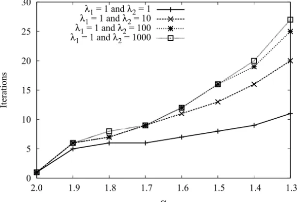
Figure 5 – Number of iterations withT ol ≤ 10−6for 17×17 nodes with biquadratic elements in the case of various combinations betweenλ1andλ2.
mesh of 17×17 nodes and 8×8 biquadratic quadrilateral elements has been used. The numerical results were performed using the following stabilizing parameters: δ1 = 1.0 and δ2 = 10.0. For the convergence of the algorithm, we imposed a tolerence of 10−6. Numerical results are shown for some com-binations of the constitutive parameters λ1 andλ2. In Figure 1 we can note the characteristic of the pseudoplastic behavior comparing the velocity profiles on x = 0.5 for the λi combinations presented. Velocity and pressure fields
are shown in Figures 2-4 for the sameλi combinations of those in Figure 1.
Petrov-Galerkin-like formulation PGhd, is shown in Figure 5, as a function of the α
power index for four Sisko fluids. It can be seen that the greater is the non-Newtonian effect, the larger is the number of iteractions required to achieve convergence, as expected for a fixed mesh. Note that even for a higher nonlin-earity (higher power indexα) convergence and stability are achieved.
6 Summary and conclusions
In this work, a consistent stabilized mixed Petrov-Galerkin-like finite element formulation in primitive variables, with continuous velocity and discontinuous pressure interpolations, has been mathematically analyzed for flows governed by the nonlinear Sisko relation. Stability, convergence and error estimates have been proven for same order interpolations of the primitive variables for any combinations whenk ≥2.
To generate the mathematical stability conditions, it was possible to split the discontinuous pressure. Only the constant by part pressure resulted as respon-sible to fulfill the LBB condition. The other part, the null mean pressure part, contributed to achieve the required ellipticity in the Scheurer’s theorem sense together with the stabilizing terms. For this formulation ellipticity was the key for the stability, since the constant part of the pressure fulfills in standard ways the LBB. It was possible from the ellipticity to provide a sufficient condition to choose the stabilizing parameters not only as a function of the quasi-newtonian constitutive parameter but considering both constitutive constants coming from the Sisko relation.
Numerical results have been presented for the benchmark driven cavity flow problem to confirm the mathematical analysis.
From the results, stability and convergence have been reached for several com-binations of the constitutive parameters of the Sisko relation, ranging from lower to highly pseudoplastic (lowα and/or highλ2) effects, although with more in-teractions in the last case.
REFERENCES
[1] R.A. Adams,Sobolev Spaces. Academic Press (1975).
[2] I. Babuška, Error bounds for finite element method. Numerische Mathematik, 16(1971), 322–333.
[3] R.B. Bird, R.C. Armstrong and O. Hassager, Dynamics of Polimeric Liquids. Wiley,Vol 1(1987).
[4] F. Brezzi,On the existence, uniqueness and approximation of saddle-point prob-lems arising from Lagrange multipliers. Revue Française d’Automatique Informa-tique et Recherche Opérationnelle, Ser. Rouge Anal. Numér.,8(1974), 129–151. [5] P.G. Ciarlet, The finite element method for elliptic problems. North-Holland
(1991).
[6] M.M. Cross, Rheology of non-Newtonian fluids: a new flow equation for pseu-doplastic systems. Journal of Colloid Science,20(1965), 417–437.
[7] M. Fortin, Old and new finite elements for incompressible flows. International Journal for Numerical Methods in Fluids,1(1981), 347–431.
[8] V. Girault and P.A. Raviart, Finite Element Methods for Navier-Stokes Equations. Theory and Applications. Springer-Verlag, Berlin (1986).
[9] T.J.R. Hughes, The Finite Element Method: Linear Static and Dynamic Finite Element Analysis. Dover Publications (2000).
[10] A.F.D. Loula and J.N.C. Guerreiro,Finite element analysis of nonlinear creeping flow. Computer Methods in Applied Mechanics and Engeneering, 79 (1990), 87–109.
[11] J. Karam Filho and A.F.D. Loula,A Non-standard application of Babuška-Brezzi theory to finite element analysis of Stokes problem. Computational and Applied Mathematics,10(1991), 243–262.
[12] B. Scheurer, Existence et approximation de points selles pour certains prob-lems non Lineaires. Revue Française d’Automatique Informatique et Recherche Opérationnelle, Ser. Rouge Anal. Numér.,11(1971), 369–400.