SELF-BOUNDED
(
A
,
B
)
-INVARIANT POLYHEDRA AND CONSTANT
REFERENCE TRACKING IN CONSTRAINED LINEAR SYSTEMS
Carlos E. T. Dórea
∗∗
Universidade Federal da Bahia, Escola Politécnica, Departamento de Engenharia Elétrica Rua Aristides Novis, 2, 40210-630 Salvador, BA, BRAZIL.
ABSTRACT
In this work the concept of self-bounded (A, B)-invariant sets is analyzed, as well as its implication in constrained controllability of discrete-time systems subject to state con-straints. Self-bounded(A, B)-invariant sets are defined and characterized. It is shown that the class of self-bounded sets contained in a given region has an infimum, that is, a self-bounded set which is contained in any set of this class. The infimal set is characterized and a numerical method is psented for its computation in the polyhedral case. These re-sults are then used to analyze the problem of constant refer-ence tracking for state constrained systems. The results are illustrated by a numerical example.
KEYWORDS: Linear systems, invariance, geometric
ap-proaches, feedback control.
RESUMO
Neste trabalho, analisa-se o conceito de conjuntos(A, B) -invariantes auto-limitados e sua implicação na restrição de controlabilidade de sistemas de tempo discreto sujeitos a res-trições lineares nos estados. Conjuntos auto-limitados são definidos e caracterizados. Mostra-se que a classe de con-juntos auto-limitados contidos em uma dada região possui um elemento ínfimo, ou seja, um conjunto auto-limitado que é contido em qualquer outro desta classe. Este conjunto ín-fimo é caracterizado e um método numérico é apresentado
Artigo submetido em 12/12/02 1a. Revisão em 10/06/03
Aceito sob recomendação do Ed. Assoc. Prof. Liu Hsu
para seu cálculo no caso poliédrico. Estes resultados são en-tão usados para se analisar o problema de rastreamento de sinais de referência constantes para sistemas sujeitos a restri-ções nos estados. Os resultados são ilustrados através de um exemplo numérico.
PALAVRAS-CHAVE: Sistemas lineares, invariância,
aborda-gem geométrica, controle por realimentação.
1
INTRODUCTION
Linear systems subject to point-wise-in-time constraints are an object of great interest for both theoreticians and prac-titioners in control systems, as constraints often arise from physical limitations on input and/or output variables. In par-ticular, the positive invarianceapproach has been success-fully used to solve a large number of problems on constrained dynamical systems. A set in the state space ispositively invariantif any trajectory originated from this set does not leave it. An overview of the literature concerning positively invariant sets and their application to the analysis and syn-thesis of control systems can be found in (Blanchini, 1999).
A key concept of this approach is that of(A, B)-invariant(or
controlled invariant) sets, which are sets that can be made positively invariant through the choice of a suitable control law (Blanchini, 1994; Dórea and Hennet, 1999) (see also (Bertsekas, 1972; Glover and Schweppe, 1971)). A typical objective in constrained control problems is to force the state trajectory to evolve inside a given region. A possible solu-tion is then to guarantee that the initial state belongs to an
and to apply a control law such that this set is positively in-variant. In general, a controlled state trajectory can leave an
(A, B)-invariant set to reach another one. However, there is a class of (A, B)-invariant sets which cannot be exited by trajectories contained in the given region. Such sets charac-terize a situation of constrained controllability and are known asself-bounded(A, B)-invariant sets.
The concept of self-boundedness was first introduced in (Basile and Marro, 1982), but limited to subspaces. In (Dórea and Hennet, 2000), this concept was extended to polyhedral sets. This choice was motivated by the fact that physical limitations inherent to the operation of actual systems very often result in linear constraints on their variables. In this work, the geometrical characterization of self-bounded sets is firstly presented. Necessary and sufficient conditions un-der which a given polyhedral set is self-bounded are shown. The infimal self-bounded set contained in a given set is then characterized and a numerical algorithm is presented for its computation in the polyhedral case.
The existence of self-bounded sets characterizes a situation of constrained controllability. This is precisely the case when one tries to design a controller so that the system output tracks a reference signal, without violating state constraints. The results on self-bounded polyhedra are then used to de-termine the set of constant reference signals which can be tracked by the constrained system. The results are illustrated by a numerical example.
Notation: In mathematical expressions, the symbol “:” stands for “such that”.0represents a null matrix of appropri-ate dimension. ker(M)represents null space of matrixM. The columns of a matrixM form agenerating setof a poly-hedral coneRif and only if there exists a nonnegative vector
ξsuch thatx= M ξ, ∀x ∈ R. Each column ofM is then called ageneratorofR. A generating set ofRis said to be a
minimal generating setif it is defined by the smallest number of generators.
2
PRELIMINARIES
Consider the linear, time-invariant, discrete-time system de-scribed by:
x(k+ 1) =Ax(k) +Bu(k), (1)
y(k) =Cx(k),
where x ∈ ℜn
is the state, u ∈ ℜm
is the control input,
y∈ ℜpis the output andkis a nonnegative integer.
A nonempty closed setΩ ⊂ ℜn
is said to bepositively in-variantwith respect to a dynamic systemx(k+1) =f(x(k))
if for all initial statex(0)∈Ωthe state trajectory remains in
Ω.
A nonempty closed setΩ⊂ ℜnis said to be(A, B)-invariant
with respect to system (1) if for all initial statex(0)∈Ωthere exists a control sequence{u(k)}such thatx(k)∈Ω∀k >0. Therefore, an(A, B)-invariant set is a set which can be made positively invariant through a suitable control action.
It can be shown that, given a convex set Ω, there exists an (A, B)-invariant set which contains all those (A, B) -invariant sets contained inΩ:
C∞(Ω)△=
supremal(A, B)-invariant set contained inΩ.
(A, B)-invariance of polyhedra for discrete-time systems was studied in e.g. (Blanchini, 1994; Dórea and Hen-net, 1999), where conditions under which a given polyhe-dron is(A, B)-invariant, as well as numerical methods for computation ofC∞
(Ω)were established.
From now on, the study will be restricted to closed convex sets containing the origin, which are the most relevant for control purposes.
A trajectory of system (1) can be forced to belong toΩif and only if the initial state belongs to an(A, B)-invariant set con-tained inΩ, hence inC∞
(Ω). LetΠbe an(A, B)-invariant set contained inΩ. In general, for any initial state belonging toΠ, it is possible not only to force the state to remain inΠ
but also to leave it with a trajectory inΩand to reach another
(A, B)-invariant set contained inΩ. On the contrary, there are(A, B)-invariant sets which cannot be exited by means of any trajectory onΩ. Such sets will be studied in next section.
3
SELF-BOUNDED
(
A
,
B
)
-INVARIANT
SETS
Definition 3.1 An(A, B)-invariant setΠcontaining the ori-gin and contained in a setΩis said to beself-boundedwith respect toΩifx(k) ∈ Π∀k > 0,∀x(0) ∈ Πand for any control sequence{u(k)}such thatx(k)∈Ω∀k >0.
In words, Π is self-bounded with respect to Ω if for any
x(0) ∈ Π, the state vector cannot leave Π through trajec-tories contained inΩ. That is, there is no control sequence {u(k)}which drives the state outsideΠ while keeping the state inΩ.
This definition extends to convex sets the concept of self-bounded(A, B)-invariant (or controlled invariant) subspaces introduced by Basile and Marro (Basile and Marro, 1982; Basile and Marro, 1992).
ex-tended spaceℜn× ℜm:
I(Π,Ω)△=
x u
:x∈Π, Ax+Bu∈ C∞(Ω)
, (2)
O(Π)△=
x u
:Ax+Bu∈Π
. (3)
Theorem 3.1 The convex setΠ⊂Ωis self-bounded(A, B)-invariant with respect toΩif and only if
I(Π,Ω)⊂ O(Π). (4)
Proof: Necessity is first proved: Since Π ⊂ C∞(Ω) and C∞(Ω)
is (A, B)-invariant, then ∀x(0) ∈ Π, there always exists a control sequence {u}(C∞(Ω)) = {u(0), u(1), u(2), ...} such that x(k) ∈ C∞(Ω) ∀k > 0
.
Suppose now that there exists
xn
un
∈ I(Π,Ω)such that
Axn+Bun ∈/ Π. Then, it is clear that forx(0) =xnthere
exists a trajectory of the state completely contained inΩ, but which leavesΠ, contradicting thereby the assumption thatΠ
is self-bounded.
Sufficiency comes from the fact that if (4) is verified, then any trajectory starting fromΠand completely contained in C∞
(Ω)(hence, inΩ) will not leaveΠ.✷
Corollary 3.1 Let{u(k)}(C∞(Ω))be any control sequence {u(0), u(1), u(2), ...}such that, x(k) ∈ C∞(Ω), ∀x(0) ∈ C∞(Ω),∀k > 0. Then, any (A, B)-invariant set Π,
self-bounded with respect toΩ, is such thatx(k)∈Π,∀x(0) ∈
Π,∀k >0,∀{u(k)}(C∞(Ω)).
Proof: It suffices to notice that any vector
x(k) u(k)
,
cor-responding to the state and the control in time k, where
x(0)∈Π,x(k)∈ C∞(Ω)
andu(k)is in{u(k)}(C∞(Ω)) , is
such that
x(k) u(k)
∈ I(Π,Ω). Therefore, if condition (4) of
self-boundedness is verified, thenx(k)∈Π∀k≥0.✷
This corollary states that any control law for whichC∞(Ω) is positively invariant is such that any self-bounded set con-tained inΩis also positively invariant under this law.
The study will now be specialized to convex polyhedra con-taining the origin, represented by sets of linear inequalities:
Ω =R[W, ζ] ={x: W x≤ζ}, ζ≥0, Π =R[G, ρ] ={x: Gx≤ρ}, ρ≥0.
whereW andGare matrices andζandρare vectors of ap-propriate dimensions. Let also the supremal(A, B)-invariant set contained inΩbe a convex polyhedron represented by:
C∞
(Ω) =R[V, ν] ={x: V x≤ν}, ν ≥0.
The hypothesis above is not always verified. C∞(Ω) may be defined by an infinite number of linear inequalities. In practice, however, this is not a serious drawback: as shown in (Blanchini, 1994), under mild assumptions,C∞
(Ω)can be arbitrarily approximated by an(A, B)-invariant polyhedron
R[V, ν].
Theorem 3.2 The convex polyhedronR[G, ρ]⊂R[W, ζ]is self-bounded(A, B)-invariant with respect toR[W, ζ]if and only if there exist matricesLandM such that:
LG+M V A=GA,
M V B=GB,
Lρ+M ν ≤ρ, L≥0, M ≥0.
(5)
Proof:See (Dórea and Hennet, 2000).
The matrix relations in (5) are linear. Self-boundedness of a polyhedron can therefore be checked through the resolution of linear programming problems as for the classical positive invariance relations (see e.g. (Hennet, 1995)).
4
THE INFIMAL SELF-BOUNDED SET
The family of(A, B)-invariant sets contained in a given con-vex set, sayΩ, is an upper semilattice with respect to the op-eration “convex hull of the union”. This property guarantees the existence, in this family of the supremal setC∞(Ω)
.
The most outstanding property of the family of self-bounded
(A, B)-invariant sets contained in a given set is to be a lattice instead of a semilattice. Hence it admits both a supremum (C∞
(Ω)) and an infimum. The existence of an infimum is guaranteed by the following property:
Property 4.1 The family of all self-bounded (A, B)-invariant sets contained in a convex set Ωis closed under intersection.
Proof: It follows immediately from the Definition 3.1. Let
Π1 andΠ2 be two self-bounded(A, B)-invariant sets
con-tained inΩ. Then it is clear that any trajectory starting from
x(0) ∈ Π1∩Π2 and contained inΩcan leave neitherΠ1
SinceΩis closed by assumption, this property guarantees the existence, in the family of self-bounded(A, B)-invariant sets contained inΩ, of an infimal element (an element which is contained in all the other elements):
C∞(Ω)△= infimal self-bounded(A, B)-invariant set
contained inΩ.
C∞(Ω) is the set defined by the intersection of all self-bounded(A, B)-invariant sets inΩ. It should be noticed that C∞(Ω) cannot be empty as it was assumed that the origin belongs to any self-bounded set.
Theorem 4.1 Consider the following sequence of sets:
C0 ={0},
Ci+1={x∈ C∞(Ω) :∃xi ∈ Ci, ui:
x=Axi+Bui}.
(6)
The infimal self-bounded(A, B)-invariant set contained inΩ is given by:C∞(Ω) = limi→∞Ci(i= 0,1,2, ...).
Proof: First we prove, by induction, thatCi ⊂ Ci+1 ∀i = 0,1,2, ...SupposeCi−1 ⊂ Ci. Then, it is clear that anyx∈
C∞
(Ω) such that there exist xi ∈ Ci−1 andui for which
x=Axi+Buibelongs toCi+1. In other words, anyx∈ Ci
belongs toCi+1. Therefore, if Ci−1 ⊂ Ci thenCi ⊂ Ci+1.
Since clearlyC0 ⊂ C1, then, by induction,Ci ⊂ Ci+1 ∀i = 0,1,2, ...
Consider now an admissible trajectory starting fromx(0)∈ C∞(Ω). A trajectory will be said to be admissible if it does not leaveΩ(henceC∞
(Ω)) ∀k > 0. SinceCi ⊂ C∞(Ω)
∀i = 0,1,2, ...thenx(0) ∈ Ci for somei. Hence,x(1) ∈
Ci+1⊂ C∞(Ω). Therefore, any admissible trajectory is such
that x(k) ∈ C∞(Ω) ∀k > 0. This proves that C∞(Ω) is self-bounded(A, B)-invariant.
Let nowC ⊂Ωbe an arbitrary self-bounded(A, B)-invariant set, and supposeCi ⊂ Cfor somei. Then,Axi+Bui ∈ C
∀xi∈ C,uisuch thatAxi+Bui∈ C∞(Ω). Therefore,x=
Axi+Bui∈ C ∀xi∈ Ci,uisuch thatAxi+Bui∈ C∞(Ω).
Hence, anyx ∈ Ci+1 also belongs toC. Therefore,Ci ⊂ C
∀ihenceC∞(Ω)⊂ C. This proves thatC∞(Ω)is infimal.✷
Ci is the set of states which can be reached from the origin
inisteps by means of a control sequence such thatx(k) ∈ C∞
(Ω) ∀k ≥ 0. Therefore, one can conclude thatC∞(Ω)
is the set of reachable states from the origin insideC∞
(Ω). It can be also noticed thatCi+1is the projection ofI(Ci,Ω)
onto the state spaceℜn.
The focus is now turned towards the computation ofC∞(Ω)
when Ω is a polyhedral set represented by R[W, ζ] and C∞
(Ω) = R[V, ν]. Let the setCi be given by: Ci = {x :
Gix≤ρi}. >From (6), the setCi+1is then given by:
Ci+1={x:∃xi, ui:x−Axi−Bui= 0,
Gixi≤ρi, V x≤ν}.
The relations definingCi+1 can be written in the following
matrix form:
I
−I 0 V
x+
−A−B
A B
Gi 0
0 0
xi
ui
≤
0 0 ρi
ν
. (7)
The dependency onxi andui in the definition ofCi+1 can
be eliminated as follows. Let the rows of matrix T =
T+ 1 T
−
1 T2
form a minimal generating set of the polyhe-dral cone defined by the vectorsw =
w+1 w
−
1 w2
, with
w1+, w1
−
, w2≥0, such that:
w+ 1 w
−
1 w2
−A−B
A B
Gi 0
=
0 0
. Then, from application of Farkas’ Lemma (Schrijver, 1987; Dórea and Hennet, 1999), ∃xi, ui such
that the first three inequalities in (7) are verified if
and only if T+ 1 T
−
1 T2
I
−I 0
x−
0 0 ρi
≤ 0
. Therefore, the set Ci+1 is given by: Ci+1 =
x:
T1+−T
−
1 V
x≤
T2ρi
ν
.
As shown in (Keerthi and Gilbert, 1987), it is possible to compute matrixT by means of Fourier-Motzkin elimination technique (Schrijver, 1987).
After suppression of redundant constraints, the polyhedral setCi+1can be written in the form: Ci+1 ={x: Gi+1x≤ ρi+1}. Algorithm (6) is then run untilCi+1 = Ci up to a
given accuracy. Since all the sets in question are polyhedra, this test can be performed via linear programming through application of Farkas’ Lemma (Hennet, 1995).
IfΩ = R[W, ζ]is an unbounded symmetrical polyhedron, then the set C∞(Ω) can have infinite directions as well. In this case, the preceding procedure is not able to com-puteC∞(Ω). One is then led to decompose its computation by “subtracting” fromΩthe minimal self-bounded(A, B) -invariant subspace contained inker(W)and applying the al-gorithm above to a polyhedron defined on a reduced order space (see (Dórea and Hennet, 1999) for further details).
5
CONSTANT
REFERENCE
TRACKING
UNDER STATE CONSTRAINTS
that the output y(k) tracks a constant reference signal r, respecting at the same time the state constraints, that is, for
allx(0)∈Ω:
(
lim
k→∞y(k) =r,
x(k)∈Ω∀k≥0.
The first specification can be achieved only if r = C¯x, wherex¯is an equilibrium point, that is, there exists au¯such that:
¯
x=Ax¯+Bu.¯
LetNBbe a matrix whose rows form a basis for the left null
space of matrixB. The set of equilibrium points is then given by:
{x¯ : NB(I−A)¯x= 0}.
Also, it is clear from the development of the preceding sec-tions that the second specificasec-tions can be achieved only if:
¯
x∈ C∞(Ω).
Indeed, ifx /¯ ∈ C∞(Ω)
, then, for somex(0) ∈ Ω, any con-trol law such thatlimk→∞x(k) = ¯xwould violate the con-straintx(k)∈Ω. Moreover, ifx¯∈ C∞(Ω)
butx /¯ ∈ C∞(Ω), then, due to the self-boundedness ofC∞(Ω), for anyx(0)∈ C∞(Ω) ⊂ Ω,x¯is not reachable from trajectories which re-spect the state constraints.
Therefore, the set of trackable constant references is given by:
YR=
r : r=Cx,¯ with NB(I−A)¯x= 0
¯
x∈ C∞(Ω)
.
Consider now the polyhedral case, for which:
Ω =R[W, ζ] ={x: W x≤ζ}, ζ≥0,
C∞(Ω) =R[G, ρ] ={x: Gx≤ρ}.
In this case:
YR={r : ∃x¯ : r−C¯x= 0,
NB(I−A)¯x= 0, Gx≤ρ}.
The relations defining YR can be written in the following
matrix form: I −I 0 0 0 r+ −C C NB(I−A)
−NB(I−A)
G ¯ x≤ 0 0 0 0 ρ . (8)
Let the rows of matrix U =
U+ 1 U
−
1 U + 2 U2U3
form a minimal generating set of the polyhedral cone
defined by the vectors u =
u+ 1 u − 1 u + 2 u −
2 u3
, with u1+, u1−, u2+, u2−, u3 ≥ 0, such that:
[u1+u1−u2+u2−u3]
−C C NB(I−A)
−NB(I−A)
G ¯ x= 0.
Then, from application of Farkas’ Lemma,∃x¯such that (8) is verified if and only if:
[U+ 1 U
−
1 U + 2 U2U3]
I −I 0 0 0 r− 0 0 0 0 ρ ≤0.
Therefore, the setYRis the polyhedron given by:
YR=
r: (U+ 1 −U
−
1 )r≤U3ρ .
The focus is now turned towards the computation of a control law which forces the system to track a given referencer ∈ YR.
It is well known that the trajectory of a system can be con-fined in an (A, B)-invariant polyhedron through a piece-wise linear state feedback control law u(k) = φ(x(k))
(Blanchini, 1994; Dórea and Hennet, 1999). If the polyhe-dron is contractive, then under this control law x(k) → 0
whenk→ ∞.
In (Blanchini and Miani, 2000) it is shown that a control law which achieves asymptotic tracking can be derived from
φ(x)by applying a translation to the state and control vari-ables, so that the new variables are given by: xˆ = x−x¯,
ˆ
u = u−u¯. Clearly, a control law such that x(k)ˆ → 0
achievesx(k)→x¯(thusy(k)→r) whenk→ ∞.
6
NUMERICAL EXAMPLE
Consider the system (1) for which:
A=
−0.8 0.2 0.5 −0.9
, B=
0 1 , C=
1−1
,
and the set of state constraintsW x(k)≤ζwith
W = 0.2 0.2
−1 −1
−1 0.35 0.25−0.5 0.6 0.1
, ζ=
The computation of the supremal(A, B)-invariant set con-tained inΩ =R[W, ζ]results inC∞(Ω) =R[V, ν]
, with:
V =
W 3.0857−0.7714
, ν=
ζ 3.8571
.
The application of the algorithm presented for computation of the infimal self-bounded(A, B)-invariant set contained in
ΩyieldsC∞(Ω) =R[G, ρ]with:
G=
0.2 0.2
−1 −1
−1 0.35 0.25 −0.5 17.5 0
−5.7143 0
, ρ=
1 1 1 1 13.8095
5.4422
.
The setsΩ,C∞
(Ω),C∞(Ω)are shown in Figure 1.
−1 −0.5 0 0.5 1 1.5 2
−2 −1 0 1 2 3 4 5
C∞(Ω)
C∞
(Ω)
Ω
Figure 1:{0} ⊂ C∞(Ω)⊂ C∞
(Ω)⊂Ω.
The computation of the set of admissible reference signals gives:
YR={r : −3.7209≤r≤0.8}.
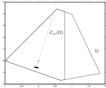
Forr= 0.5, the correspondingx¯andu¯are:
¯ x=
−0.0625
−0.5625
, u¯=−1.0375.
It turns out that, in this example, closed-loop positive invari-ance ofC∞(Ω)can be achieved through linear state feedback
u(k) =F x(k)(see in e.g. (Hennet, 1995) details on how it
−1 −0.5 0 0.5 1 1.5 2
−2 −1 0 1 2 3 4 5
C∞(Ω)
Ω
Figure 2: Ω,C∞(Ω), admissiblex¯and the trajectory of the state.
can be checked via linear programming). Then, the appli-cation of the procedure based on variable translation, sug-gested in (Blanchini and Miani, 2000) for the computation of a control law such that the system can trackr = 0.5, gives the linear state feedback: u(k) = F(x(k)−x) + ¯¯ u, with
F =
0.0079 0.8178
.
In Figure 2 the setsΩ,C∞(Ω)and the set of admissiblex¯are shown, as well as a trajectory of the state under the control law computed above, with null initial state. In Figure 3 the responsey(k)is shown.
It can be noticed that in this examplex¯andu¯are unique for the given referencer. However, this is not true in the general case. As suggested by one of the reviewers, this freedom on the choice ofx¯andu¯could be used to optimize the compu-tation of the tracking control law, in the sense of achieving other control goals.
7
CONCLUSIONS
This work presented the concept of self-bounded (A, B) -invariant sets of the state space for discrete-time systems. The existence of such sets implies limitations in the control-lability of trajectories confined in a given set. Self-bounded polyhedral sets were geometrically and analytically charac-terized.
Linear Simulation Results
Time (sec)
Amplitude
0 5 10 15 20 25 30 35 40 45 50
0 0.1 0.2 0.3 0.4 0.5 0.6
Figure 3: Time responsey(k).
characterized and a numerical method was presented for its computation in the polyhedral case.
Finally, it was shown how this concept can be applied in the study of a tracking problem for state constrained linear sys-tems. The set of the constant reference signals which can be tracked was then characterized.
Although only state constraints have been treated here, as shown in (Dórea and Hennet, 2000), control constraints as well as persistent disturbances can be easily casted in the pre-sented framework.
ACKNOWLEDGEMENTS
This work was partially supported by CNPq, Brazil, under grants # 301439/1997-4 and 471448/01-0.
REFERENCES
Basile, G. and Marro, G. (1982). Self-bounded controlled invariant subspaces: a straightforward approach to constrained controllability, J. Optimiz. Theory Appl.
38: 71–81.
Basile, G. and Marro, G. (1992).Controlled and Conditioned Invariants in Linear System Theory, Prentice-Hall.
Bertsekas, D. P. (1972). Infinite-time reachability of state-space regions by using feedback control,IEEE Trans. Automat. Contr.17(5): 604–613.
Blanchini, F. (1994). Ultimate boundedness control for un-certain discrete-time systems via set-induced Lyapunov
functions, IEEE Trans. Automat. Contr. 39(2): 428– 433.
Blanchini, F. (1999). Set invariance in control, Automatica
35(11): 1747–1767.
Blanchini, F. and Miani, S. (2000). On the tracking problem for constrained linear systems,Proc. 14th International Symposium of Mathematical Theory of Networks and Systems, Perpignan, France.
Dórea, C. E. T. and Hennet, J.-C. (1999). (A, B)-invariant polyhedral sets of linear discrete-time systems,J. Opti-miz. Theory Appl.103(3): 521–542.
Dórea, C. E. T. and Hennet, J.-C. (2000). Self-bounded
(A, B)-invariant polyhedra of discrete-time systems,
Proc. 39th IEEE Conf. Decision Contr., Sydney, Aus-tralia, pp. 3163–3168.
Glover, J. D. and Schweppe, F. C. (1971). Control of lin-ear dynamic systems with set constrained disturbances,
IEEE Trans. Automat. Contr.16(5): 411–423.
Hennet, J.-C. (1995). Discrete-time constrained linear sys-tems,inC. Leondes (ed.), Control and Dynamic Sys-tems, Vol. 71, Academic Press, pp. 157–213.
Keerthi, S. S. and Gilbert, E. G. (1987). Computation of minimum-time feedback control laws for discrete-time systems with state-control constraints,IEEE Trans. Au-tomat. Contr.32(5): 432–435.