ERROR IDENTIFICATION AND COMPENSATION IN LARGE
MANIPULATORS WITH APPLICATION IN CANCER PROTON THERAPY
Meggiolaro, M.A.
∗S. Dubowsky
†C. Mavroidis
‡∗PUC-Rio, Dept. of Mechanical Engineering - Rua Marquês de São Vicente, 225 - Gávea, Rio de Janeiro, RJ
†MIT, Dept. of Mechanical Engineering, 77 Massachusetts Ave, Cambridge, MA 02139, USA
‡Rutgers University, Dept. of Mechanical and Aerospace Engineering, 98 Brett Road, Piscataway, NJ 08854, USA
ABSTRACT
Important robotic tasks could be effectively performed by powerful and accurate manipulators. However, high accu-racy is generally difficult to obtain in large manipulators ca-pable of producing high forces due to system elastic and ge-ometric distortions. A method is presented to identify the sources of end-effector positioning errors in large manip-ulators using experimentally measured data. The method does not require explicit structural modeling of the system. Both geometric and elastic deformation positioning errors are identified. These error sources are used to predict, and compensate for, end-point errors as a function of configu-ration and measured forces, improving the system absolute accuracy. The method is applied to a large high-accuracy medical robot. Experimental results show that the method is able to effectively correct for the system errors.
KEYWORDS: Robot calibration, Flexible arms, Medical
sys-tems.
RESUMO
Importantes tarefas robóticas poderiam ser eficientemente
Artigo submetido em 02/12/02 1a. Revisão em 12/05/03
Aceito sob recomendação do Ed. Assoc. Prof. Paulo E. Miyagi
executadas por manipuladores potentes e precisos. No en-tanto, alta precisão absoluta é geralmente difícil de ser ob-tida em grandes manipuladores capazes de produzir forças de alta intensidade, devido às distorções elásticas e geomé-tricas do sistema. Um método é apresentado para identificar, através de medições indiretas, as fontes de erro de posiciona-mento da extremidade de grandes manipuladores. O método não requer uma modelagem estrutural explícita do sistema. Ambos os erros geométricos e elásticos de posicionamento são identificados. Esses valores são usados para predizer e compensar os erros da extremidade do robô em função da configuração e de forças medidas, melhorando a precisão ab-soluta do sistema. O método é aplicado a um grande robô médico de alta precisão. Resultados experimentais demons-tram que o método é capaz de corrigir eficientemente os erros de posicionamento do sistema.
PALAVRAS-CHAVE: Calibragem de robôs, manipuladores
flexíveis, sistemas médicos.
1
INTRODUCTION
medi-cal treatment (Vaillancourt et al. 1994; Flanz 1996; Hamel et al. 1997). In these applications, a large robotic system is of-ten needed to have very fine precision. Its accuracy specifica-tions may be very small fracspecifica-tions of its size. Achieving such high accuracy is difficult because of the manipulator’s size and its need to carry heavy payloads. Further, many tasks, such as space applications, require systems to be lightweight, and thus structural deformation errors can be large.
In such systems, two principal error sources create significant end-effector errors. The first is kinematic errors due to the non-ideal geometry of the links and joints of manipulators, such as errors due to machining tolerances. These errors are often called geometric errors. Task constraints often make it impossible to use direct end-point sensing in a closed-loop control scheme to compensate for these errors. Therefore, there is a need for model-based robot calibration.
The second error source that can limit the absolute accuracy of a large manipulator is the elastic errors due to the distor-tion of a manipulator’s mechanical components under large task loads or even its own weight. Classical error compensa-tion methods cannot correct the errors in large systems with significant elastic deformations, because they do not explic-itly consider the effects of task forces and structural compli-ance. Methods have been developed to deal with this prob-lem (Drouet et al. 1998), however they depend upon lenghty analytical models of the manipulator structural properties.
In this work a method that compensates for the position and orientation errors caused by geometric and elastic errors in large manipulators is discussed. The method, called here Geometric and Elastic Error Compensation (GEC), explic-itly considers the task load dependency of the errors, model-ing both deformation and more classical geometric errors in a unified and simplified manner. A set of experimentally mea-sured positions and orientations of the robot end-effector and measurements of the payload wrench are used to calculate the robot “generalized” errors without using an explicit ma-nipulator elastic model. Without the need of an explicit elas-tic model, it is feasible to completely automate the analyelas-tical derivation of the required identification matrices. General-ized are called the errors that characterize the relative po-sition and orientation of frames defined at the manipulator links. They are determined from measured data as a function of the system configuration and the task wrench. Knowing these generalized errors the manipulator end-effector errors are used to compensate for robot errors at any configuration. In the GEC method each generalized error parameter can be represented as a function of only a few of the system vari-ables. As a result, the number of measurements required to characterize the system is significantly smaller than ex-pected.
PPS
Rotating
Gantry
Proton Beam
Nozzle
Figure 1: The PPS and the Gantry
Figure 2: The Patient Positioning System
The required absolute positioning accuracy of the PPS is 0.5 mm. This accuracy is critical as larger errors may be dan-gerous to the patient (Rabinowitz 1985). The required ac-curacy is roughly 10−4
of the nominal dimension of system workspace. This is a greater relative accuracy than most in-dustrial manipulators. In addition, FEM studies and experi-mental results show that with a changing payload (between 1 and 300 pounds) and changing configuration the end-effector errors due to elastic deformations and geometric errors are of the order of 6-8 mm. Hence the accuracy is 12 to 16 times the system specification (Mavroidis et al. 1997). However, since the repeatability error of the PPS, defined here as how well the system returns to certain arbitrary configurations, is less than 0.15mm, it is a good candidate for a model based error correction method.
The GEC calibration method was applied to the PPS with a force/torque sensor built into the system to measure the wrench applied by the patient’s weight. It is found that us-ing only 450 calibration measurements the end-point errors could be reduced to well within the required specification. In fact, experimental results show that the maximum error was reduced by a factor of 18.
2
ANALYTICAL BACKGROUND
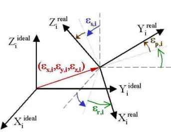
Physical errors cause the geometric parameters of a manipu-lator to be different from their ideal values (Roth et al. 1986). As a result, the frames defined at the manipulator joints are slightly displaced from their expected, ideal locations, cre-ating significant end-effector errors. The position and ori-entation of a frame Freal
i with respect to its ideal location Fideal
i is represented by a 4x4 homogeneous matrixEi. The translational part of matrixEi is composed of the 3 coordi-natesεx,i,εy,i andεz,i(along the X, Y and Z axes respec-tively, defined using the Denavit-Hartenberg representation), see Fig. 3. The rotational part of matrix Ei is the result of the product of three consecutive rotations εs,i, εr,i, εp,i around the Y, Z and X axes respectively (also shown in Fig. 3). These are the Euler angles of Freal
i with respect to F ideal i . The subscripts s, r, and p represent spin (yaw), roll, and pitch, respectively. The 6 parametersεx,i,εy,i,εz,i,εs,i,εr,i and
εp,iare called generalized error parameters, which can be a function of the system geometry and joint variables. For ann
degree of freedom manipulator, there are 6(n+1) generalized errors which can be written in the form of a 6(n+1) x 1 vector
ε= [εx,0, . . . , εx,i,εy,i,εz,i,εs,i,εr,i,εp,i,. . . ,εp,n], withi ranging from 0 ton, assuming that both the manipulator and the location of its base are being calibrated. The general-ized errors that depend on the system geometry, the system task loads and the system joint variables can be calculated from the physical errors link by link. Note that actual sys-tem weight effects can be included in the model as a simple
function of joint variables.
Figure 3: Definition of the Translational and Rotational Gen-eralized Errors for ithLink
Since the generalized errors are small, the end-effector posi-tion and orientaposi-tion error∆Xcan be defined as the 6x1 vec-tor that represents the difference between the real position and orientation of the end-effector and the ideal one:
∆X=Xreal−Xideal (1)
whereXrealandXidealare the 6x1 vectors composed of the three positions and three orientations of the end-effector ref-erence frame in the inertial refref-erence system for the real and ideal cases, respectively. After linearization, the end-effector error can be represented by the following linear equation:
∆X=Jeε (2)
whereJeis the 6x6(n+1) Jacobian matrix of the end-effector error∆Xwith respect to the elements of the generalized er-ror vectorε, also known as Identification Jacobian matrix (Zhuang et al. 1999). As with the generalized errors,Je de-pends on the system configuration, geometry and task loads.
If the generalized errors,εscan be found from calibration
measurements, then the correct end-effector position and ori-entation error can be calculated using Eq. (2) and be compen-sated. To calculate the generalized errorsεit is assumed that some components of vector∆Xcan be measured at a finite number of different manipulator configurations.
(2)mtimes:
∆Xt=
∆X1
∆X2
... ∆Xm
=
Je(q1)
Je(q2)
... Je(qm)
·
ε=Jt·ε (3)
where∆Xtis themx 1 vector formed by all measured vec-tors ∆X at m different configurations andJt is the 6m x 6(n+1) matrix formed by themIdentification Jacobian ma-trices Je at m configurations, called here Total Identifica-tion Jacobian. To compensate for the effects of measurement noise, the number of measurementsmis, in general, much larger thann.
If the generalized errorsεare constant, then a unique least-squares estimateˆecan be calculated (Roth et al. 1986):
ˆ ε=¡
JtTJt¢
−1
JtT ·∆Xt (4)
However, if the Identification Jacobian matrixJe(qi) con-tains linearly dependent columns, Eq. (4) will produce esti-mates with poor accuracy (Hollerbach et al. 1996). This oc-curs when there is redundancy in the error model, in which case it is not possible to distinguish the error contributed by each generalized error component, even if specific measure-ment configurations are considered. Orthogonal matrix de-composition can be used in these cases to improve the nu-merical accuracy of this approach. An analytical method to eliminate the redundant parameters has been presented by (Meggiolaro and Dubowsky 2000). Conventional calibration methods also cannot be successfully applied when some of the generalized errors depend on the manipulator configura-tionqor the end-effector wrenchw, namelyε(q,w), such as when elastic deflections that depend on the configuration and applied forces at the end-effector are significant. A method is presented below for finding the generalized errors (ε) in the presence of elastic deformations combined with geometric errors.
3
GEOMETRIC
AND
ELASTIC
ERROR
COMPENSATION
In the GEC method (Geometric and Elastic Error Compensa-tion), elastic deformation and classical geometric errors are considered in a unified manner. The method can identify and compensate for both types of error, without an elastic model of the system. To apply the GEC method, the error model is extended to explicitly consider the task loading wrench and configuration dependency of the errors.
For a system with significant geometric and elastic errors, the generalized errorsεare a function of the manipulator con-figurationq and the end-effector wrenchw, or ε(q,w). To
predict the endpoint position of the manipulator for a given configuration and task wrench, it is necessary to calculate the generalized errors from a set of offline measurements. The complexity of these calculations can be substantially reduced if the generalized errors are parameterized using polynomial functions. The ithelement of vectorεis approximated by a polynomial series expansion of the form:
ε∗
i = ni
P
j=1
ci,j·fi,j(q,w),
fi,j(q,w)≡(wmj)
a0,j·(qa1,j
1 ·q a2,j
2 ·...·q an,j
n ) (5)
whereniis the number of terms used in each expansion, ci,j are the polynomial coefficients, wmjis an element of the task wrenchw, and q1, q2, ..., qnare the manipulator joint param-eters. It has been found that good accuracy can be obtained using only a few terms ni in the above expansion (Meggi-olaro et al. 1998). From the definition of the generalized errors, the errors associated with theithlink depend only on the parameters of the ithjoint. If elastic deflections of link i are considered, then the generalized errors created by these deflections would depend on the weight wrench wi applied at the ithlink. For a serial manipulator, this wrench is due to the wrench at the end-effector and to the configuration of the links after theith. Hence, the wrench w
idepends only on the joint parameters qi+1,...,qn. Thus, the number of terms in the products of Eq. (5) is substantially reduced. Each general-ized error parameter is then represented as a function of only a few of the system variables, greatly reducing the number of measurements required to characterize the system using the GEC method.
The constant coefficients ci,jare grouped into one vectorc, becoming the unknowns of the problem. The total number of unknown coefficients, callednc, is the sum of the number of terms used in Eq. (5) to approximate each generalized error, i.e. nc = Σni. The nc functions fi,j(q,w) are then incorporated into the Identification Jacobian matrixJefrom Eq. (2):
∆X=Je(q)·ε(q,w)≡He(q,w)·c (6)
whereHeis the (6 xnc)Jacobian matrix of the end-effector error ∆X with respect to the polynomial coefficients ci,j. The matrixHe, called here Extended Identification Jacobian matrix, can be obtained from Eqs. (5) and (6):
He(q,w)≡[J1·f1,1, . . . ,J1·f1,n1, . . . ,
Ji·fi,1,Ji·fi,2, . . . , Ji·fi,ni, . . .] (7)
whereJiis the column of matrixJeassociated to the gener-alized error componentεi.
Eq. (4), completing the identification process, see Eq. (8). Once the constant polynomial coefficients,c, are identified, the end-effector position and orientation error∆Xcan be cal-culated and compensated using Eq. (6).
ˆ
c= (HTeHe) −1
HTe ·∆X (8)
Finally, it must be emphasized that the GEC model has the advantage of modeling non-linear elasticity, due to its poly-nomial nature. The polypoly-nomial approximation would only be a model of linear elasticity if the order of the polynomial was limited to three (relating the joint parameters, or order one relating the payload wrench), and if these polynomial coefficients were related among themselves in the same way as in the analytical results for simple beam bending. How-ever, the polynomial expansion can include additional terms, being able to model general non-linear (or linear) elasticity, combined with a general formulation for geometric errors that may vary in their own frames (and thus not limited to constant geometric errors).
4
APPLICATION TO THE PATIENT
POSI-TIONING SYSTEM
The PPS is a six degree of freedom robot manipulator (see Fig. 2) built by General Atomics (Flanz 1996). The first three joints are prismatic, with maximum travel of 225cm, 56cm and 147cm for the lateral (X), vertical (Y) and longitu-dinal (Z) axes, respectively. The last three joints are revolute joints. The first joint rotates parallel to the vertical (Y) axis and can rotate±90˚. The last two joints are used for small corrections around an axis of rotation parallel to the Z (roll) and X (pitch) axes, and have a maximum rotation angle of
±3˚. The manipulator "end-effector"is a couch, supporting the patient in a supine position, accommodating patients up to 188cm in height and 300lbs in weight in normal operation.
The intersection point of the proton beam with the gantry axis of rotation is called the system isocenter. The treatment volume is defined by a treatment area on the couch of 50cm x 50cm and a height of 40cm (see Figure 2). This area covers all possible locations of treatment points (i.e. tumor loca-tions at a patient). The objective is that the PPS makes any point in this volume be coincident with the isocenter at any orientation.
The joint parameters of the PPS are the displacements d1, d2, d3of the three prismatic joints and the rotationsθ,α,β
of the three rotational joints. A 6 axis force/torque sensor is placed between the couch and the last joint. By measuring the forces and moment at this point, it is possible to calculate the patient weight and the coordinates of the patient center of gravity. The system motions are very slow and smooth due to safety requirements. Hence, the system is quasi-static, and
its dynamics do not influence the system accuracy and are neglected.
The accuracy of the PPS was measured with a position ac-curacy of approximately 0.04mm using a Leica 3D Laser Tracking System. These measurements were to evaluate the PPS repeatability, the nonlinearity of its weight-dependent deflections, the inherent uncompensated PPS accuracy, and the method developed above.
Three targets were placed about 10mm above the couch. For more than 700 different configurations of the PPS and dif-ferent weights the location of the three targets is measured. From the system kinematic model with no errors, the ideal coordinates of the Nominal Treatment Point (NTP), defined as the location of a tumor on a patient, were calculated and subtracted from the experimentally measured values to yield the vector∆X(q,w). Then, 450 measurements were used to evaluate the basic uncompensated accuracy of the PPS and the accuracy of the compensation method described above. Two different payloads were used: one with no weight and another with a 70 kg weight at the center of the treatment area. The PPS configurations used were grouped into two sets:
Set a)Treatment Volume. The 8 vertices of the treatment volume (see Figure 2) are reached with the NTP with angle
θtaking values from -90˚ to 90˚ with a step of 30˚, for a total of 112 configurations.
Set b)Independent Motion of Each Axis. Each axis is moved independently while all other axes are held at the home (zero) values. The step of motion for d1 is 50 mm, for d220 mm, for d325mm and forθ5˚, resulting in 338 configurations.
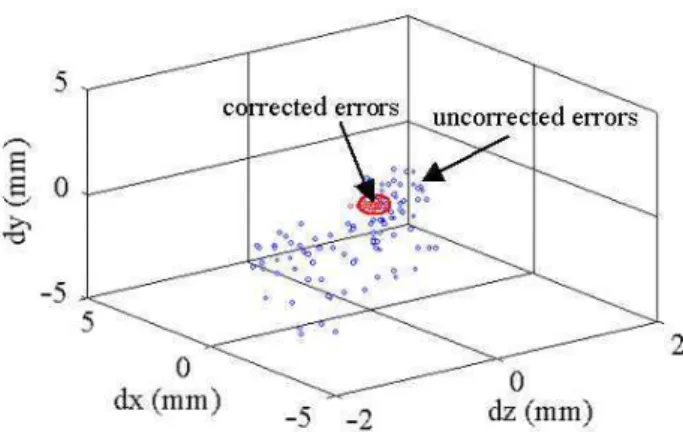
The PPS uncompensated accuracy combining the two sets is shown in Figure 4. The data points represent the position-ing errors of NTP. It is clearly seen that in spite of the high quality of the PPS physical system, its uncompensated accu-racy is on the order of 10mm. This is approximately 20 times higher than the specification of±0.50mm.
Figure 4: Measured and Residual Errors After Compensation
In implementing the computation method a general nonlin-ear function of the wrenchwcan be used. To help establish this function, the behavior of the PPS positioning errors for different payload weights was examined with measurements made at the home (zero) configuration. The weights ranged from 0 to 300 lbs in steps of approximately 25 lbs. The re-sults showed that the positioning errors of the PPS are nearly linear with the payload weight. The least square error is less than 0.1mm for the linear fit. Hence the generalized errors were taken as linear functions of the system wrench in Eq. (5).
The generalized errors are then calculated with Eq. (4) using the configurations of set (b) (independent motion of its axes) and half of the treatment volume data (set a). For a Pentium PC 300MHz, the computing time was less than one minute. The PPS is then commanded to go to compensated points for the remaining configurations of set (a). The residual posi-tioning errors of the PPS after compensation for these points are shown in Fig. 4. The residual errors are enclosed in a sphere of 0.38 mm radius which is smaller than the accuracy specification. The required number of data points for this cal-culation was less than 400. Hence the compensation method used in this paper enables the system to meet its specifica-tion. It is now a key element in MGH’s operational software. Since the remaining errors after calibration using 400 points were comfortably under 0.5mm, a significantly smaller num-ber of poses could have been used in the calibration. In fact, applying the presented calibration method to a subset of only 125 measurement poses of the Patient Positioning System re-sulted in a maximum residual error of 0.49mm. This abso-lute accuracy meets the specification, while significantly less than 400 measurement points were necessary. This number is indeed much smaller than it might be expected, considing that not only elastic deformations, but also geometric er-rors that vary in their own frames (such as a quasi-sinusoidal shape for the rail errors on the prismatic base, as discussed below), are present in the system. However, the calibration
error dependence on the number of measurement poses has not been addressed in this work.
One of the main advantages of the GEC methodology is the ability to model non-linearities or any other repeatable error source that can be represented as a function of the system parameters and of the payload wrenches. Since any differ-entiable analytical expression can be represented as a poly-nomial series, the method is able to identify errors that other calibration methods (which only model elastic deformations and geometric errors constant in their frames) can’t. In par-ticular, the errors along the Patient Positioner’s lateral rail had an approximately sinusoidal shape (as it was expected from the respective manufacturing process, due to eccentric-ities in its machining), which turned out to be an important error source in this system. These errors were identified through the presented methodology using polynomial expan-sions with relatively few terms (about 8th order).
In addition, the GEC method has an advantage of automat-ically accounting for the elastic deformations due to link masses. The polynomial terms that are a function of the system configuration (but not of the task wrench w) are the ones that account for the contribution of the link masses to the varying end-effector elastic errors. Since the link masses are constant (only the associated moments are variable), the constant polynomial coefficients associated with these terms will automatically account for these masses. These errors are clearly configuration-dependent, as expected, since the poly-nomial terms that multiply these constant mass coefficients are a function of the system configuration. Therefore, all link masses are implicitly identified, and their associated elastic errors are automatically compensated for.
5
CONCLUSIONS
In this work, a method is discussed to compensate the posi-tioning end-effector errors of large manipulators with signif-icant task loads. Both geometric and elastic errors are con-sidered without requiring an explicit elastic model of the sys-tem. The method has been applied experimentally to a high-accuracy large medical manipulator. The results showed that the basic accuracy of the manipulator exceeded its speci-fications, but after applying the method to compensate for end-effector errors the accuracy specifications are met. The method is now a key element of the software used to treat cancer patients.
ACKNOWLEDGEMENTS
REFERENCES
Drouet, P., Dubowsky, S. and Mavroidis, C. (1998). Com-pensation of Geometric and Elastic Deflection Errors in Large Manipulators Based on Experimental Measure-ments, Proceedings of the 6th Int. Symposium on Ad-vances in Robot Kinematics, Austria, pp. 513-522.
Flanz, J. (1996). Design Approach for a Highly Accurate Patient Positioning System for NPTC, Proceedings of
thePTOOG XXVandHadrontherapy Symposium,
Bel-gium, pp. 1-5.
Hamel W., Marland S. and Widner T. (1997). A Model-Based Concept for Telerobotic Control of Decontam-ination and Dismantlement Tasks, Proceedings of the 1997 IEEE International Conference of Robotics and
Automation, Albuquerque, New Mexico.
Hollerbach, J.M., Wampler, C.W. (1996). The Calibration Index and Taxonomy for Robot Kinematic Calibration Methods, International Journal of Robotics Research, Vol. 15, No. 6, pp. 573-591.
Mavroidis, C., Dubowsky, S., Drouet, P., Hintersteiner, J., Flanz, J. (1997). A Systematic Error Analysis of Robotic Manipulators: Application to a High Perfor-mance Medical Robot, Proceedings of the1997 IEEE
Int. Conference of Robotics and Automation,
Albu-querque, New Mexico, pp. 980-985.
Meggiolaro, M., Mavroidis, C., Dubowsky, S. (1998). Iden-tification and Compensation of Geometric and Elastic Errors in Large Manipulators: Application to a High Accuracy Medical Robot, Proceedings of the25th
Bi-ennial Mechanisms Conference, ASME, Atlanta.
MEGGIOLARO, M., DUBOWSKY, S. (2000). ANANALYT -ICALMETHOD TOELIMINATE THEREDUNDANTPA -RAMETERS INROBOTCALIBRATION, PROCEEDINGS OF THEInternational Conference on Robotics and
Au-tomation(ICRA ’2000), IEEE, SANFRANCISCO,PP.
3609-3615.
Rabinowitz, I. (1985). Accuracy of Radiation Field Align-ment in Clinical Practice, International Journal of Radi-ation Oncology, Biology and Physics, Vol.11, pp.1857-1867.
Roth, Z.S., Mooring, B.W., Ravani, B. (1986). An Overview of Robot Calibration,IEEE Southcon Conference, Or-lando, Florida, pp. 377-384.
Vaillancourt C. and Gosselin, G. (1994). Compensating for the Structural Flexibility of the SSRMS with the SPDM, Proceedings of the International Advanced Robotics Program, Second Workshop on Robotics in
Space, Canadian Space Agency, Montreal, Canada.