Sba Controle & Automação vol.22 número6

(1)

STABILITY ANALYSIS OF TAKAGI-SUGENO FUZZY SYSTEMS VIA

LMI: METHODOLOGIES BASED ON A NEW FUZZY LYAPUNOV

FUNCTION

Leonardo Amaral Mozelli

∗

mozelli@ufsj.edu.br

Reinaldo Martinez Palhares

‡† palhares@cpdee.ufmg.br

∗_{Universidade Federal de S˜}_{ao Jo˜}_{ao del-Rei}

Departamento das Engenharias de Telecomunica¸c˜oes e Mecatrˆonica Rod. MG 443, Km 7 - Campus Alto Paraopeba

36420-000 - Ouro Branco - MG - Brasil

†_{Universidade Federal de Minas Gerais}

Departamento de Engenharia Eletrˆonica Av. Antˆonio Carlos 6627 - Pampulha 31270-010 - Belo Horizonte - MG - Brasil

‡ _{Autor para contato.}

RESUMO

An´alise da estabilidade de sistemas fuzzy de Takagi-Sugeno via LMI: Metodologia baseda numa nova fun¸c˜ao de Lyapunov fuzzy

A análise de estabilidade de sistemas fuzzy TS pode ser aprimorada com o uso de fun¸cões de Lyapunov fuzzy, uma vez que as mesmas são parametrizadas por fun¸cões de pertinência e podem definir melhor a ca-racter´ıstica variante no tempo de tais sistemas através do uso da in-forma¸cão relacionada à primeira derivada temporal das fun¸cões de pertinência. Neste trabalho uma fun¸cão de Lyapunov fuzzy aperfei¸coada é usada com o intuito de se desenvolver condi¸cões de estabilidade que avaliam tam-bém a segunda derivada temporal das fun¸cões de per-tinência, aprimorando a caracteriza¸cão do aspecto vari-ante no tempo de sistemas TS. Novos testes no formato de LMIs são desenvolvidos usando diferentes estratégias para incorporar tais derivadas e empregando algumas ferramentas numéricas que desacoplam as matrizes do

Artigo submetido em 06/03/2011 (Id.: 01288) Revisado em 11/05/2011, 01/10/2011

Aceito sob recomenda¸c˜ao do Editor Associado Prof. Carlos Roberto Minussi

sistema daquelas da fun¸cão de Lyapunov fuzzy. Exem-plos numéricos ilustram a eficácia dessas metodologias.

PALAVRAS-CHAVE_{: sistemas fuzzy Takagi-Sugeno,}

De-sigualdades Matriciais Lineares, An´alise de Estabilidade

ABSTRACT

(2)

KEYWORDS_{: Takagi-Sugeno fuzzy systems, Linear}

Ma-trix Inequalities, Stability analysis

1 INTRODUCTION

Stability analysis and control design for Takagi-Sugeno fuzzy systems (Takagi and Sugeno, 1985) have been rou-tinely formulated as feasibility and optimization prob-lems in LMI (Linear Matrix Inequalities) form (Tanaka and Wang, 2001). Recently powerful SOS formulations have been proposed by Tanaka et al. (2009) enhancing numerical performance. Nonetheless, a source of conser-vativeness that remains is the choice of an appropriate candidate Lyapunov function.

For some time it has been noticed that parameter-ized Lyapunov functions are a good choice to deal with time-varying systems, deserving attention some semi-nal works on this subject (Gahinet et al., 1996; Feron et al., 1996; Fierro et al., 1996). The idea is to use an affine combination of quadratic functions (xT_{P x}_{), which} individually are not necessarily Lyapunov, parameter-ized by uncertain time-varying parameters. This com-bination leads to a Lyapunov function. The fuzzy Lya-punov functions proposed in Jadbabaie (1999) and Rhee and Won (2006) fall into this category but the parame-terization is given in terms of the membership functions.

The reason because this parametrization reduces con-servativeness is twofold. To guarantee stability in the Lyapunov sense the information regarding the first time-derivative of the parameters must be taken into account. This is an advantage in comparison with quadratic sta-bility where regardless the time-varying feature of a system stability is imposed to it for arbitrary rates of change. In other words, quadratic stability consid-ers only polytopic characteristic. Another reason is that using multiple Lyapunov functions more degrees of freedom are granted for the LMI problem whereas for quadratic stability a single Lyapunov function is avail-able.

The fuzzy Lyapunov function in Jadbabaie (1999) and in Tanaka et al. (2003) posses both these features whereas the function used in Rhee and Won (2006) and in Mozelli, Palhares, Avellar and dos Santos (2010) does not. Rhee and Won (2006) proposed a line in-tegral fuzzy Lyapunov function, similar to those ob-tained through the variable gradient method for nonlin-ear systems (Haddad and Chellaboina, 2008), that does not rely on the first time-derivative of the membership functions. Although it is a multiple Lyapunov func-tion, which is an improvement and includes quadratic stability as a particular case, it can be noticed that

for some systems the missing information regarding pa-rameter variation can produce more conservative results (Mozelli, Palhares, Souza and Mendes, 2009; Mozelli, Palhares and Avellar, 2009).

Motivated by the relevance inherent to information re-garding the time-derivative of the membership functions a new Lyapunov function is employed in this paper pa-rameterized not only by the membership functions but also by the first time-derivative of them. By doing that the information concerning the second time-derivative of the membership functions becomes available to de-scribe better the time-varying characteristic of TS sys-tems. The new function was previously presented in a conference paper (Mozelli and Palhares, 2010) and good results were achieved. In this paper extra numerical tools are employed to reduce conservativeness even more as the computational effort is kept low. Numerical ex-amples are performed to illustrate the advantages in us-ing this new kind of function together with the strategies discussed in Mozelli, Palhares and Mendes (2010).

1.1 Notation

The notation used throughout is standard. The super-scriptT _{indicate transposition of vectors and matrices;} for matrices M >0 (≥0) indicates that M is positive definite (nonnegative definite); M(i,j) denotes the i-th

line andj-th column element; the subsets{1,2, . . . , r} ⊂

N∗_, _{₁_,₂_{, . . . , p}_{} ⊂}_N∗ _and _{₁_,₂_{, . . . , m}_{} ⊂}_N∗ _are rep-resented byR,P andM, respectively.

2 FUNDAMENTS ON TS MODELS

Takagi-Sugeno (TS) dynamic fuzzy systems are de-scribed by means of a set of fuzzy rules (Tanscheit et al., 2007; Teixeira and Assun¸c˜ao, 2007)

Ri: If z1(t) isM1i and · · · andzp(t) isMip

Then x˙(t) =Aix(t)

(1)

where the state vector isx(t)∈Rn_{; the number of local} models and fuzzy rules Ri is given by r; Ai are real matrices of appropriate dimension; for this model, the premise variables vector isz(t) = [z1(t)· · ·zp(t)] and the input sets are indicated byMi

j, i∈ R, j∈ P.

(3)

˙

x(t) =A(h)x(t), (2)

with

A(h),

r X

i=1

hi(z(t))Ai, h= [h1(z(t)) · · · hr(z(t))],

where hi(z(t)) are the normalized membership func-tions:

hi(z(t)),

ωi(z(t)) Pr

i=1ωi(z(t))

,

withωi(z(t)) given by product fuzzy inference

ωi(z(t)), p Y

j=1

µi j(zj(t)).

The grades of membership of the premise variables in the respective fuzzy setsMi

jare given asµij(zj(t)). The normalized membership functions satisfy the following properties

hi(z(t))∈[0,1], r X

i=1

hi(z(t)) = 1,

r X

i=1

˙

hi(z(t)) = 0, r X

i=1

¨

hi(z(t)) = 0.

(3)

From now on to avoid clutter the time dependency of some variables is dropped out. For instance,hi(z(t)) is replaced byhi.

3 FUZZY LYAPUNOV FUNCTION

PA-RAMETERIZED

BY

MEMBERSHIP

FUNCTIONS

AND

THEY

TIME-DERIVATIVES

The fuzzy Lyapunov function proposed in Mozelli and Palhares (2010) is given by a double parametrization, using affine combinations of quadratic functions. One set is parameterized by the membership functions and another parameterized by they first time-derivatives:

V(x, h,h˙) =xThP1(h) +P2( ˙h)ix, (4)

where

P1(h),

r X

i=1

hiPi1, P2( ˙h), r X

i=1

˙

hiPi2. (5)

Notice that the proposed function is indeed a Lyapunov one since

• V(x, h,h˙)∈ C1_{, case}_h

i(z(t))∈ C2

• V(0, h,h˙) = 0

• kx(t)k → ∞ ⇒ V(x, h,h˙) → ∞ (radially un-bounded)

It remains to ensure thatV(x, h,h˙)>0,∀x(t)6= 0 being sufficient to meet the following conditions

P1

i +

r X

k=1

˙

hkPk2>0, ∀i∈ R (6)

3.1 On the time-derivative of the

member-ship functions

There is more than one way to recast conditions involv-ing the time-derivatives of the membership functions into the LMI framework. The simplest but more conser-vative form is to consider the worst case scenario taking only the upper bounds, as done in Tanaka et al. (2003).

Due to the properties (3), the time-derivative of the membership functions belong into the convex polytope defined by

Ωω , co{v1, v2, . . . , vm}

= {vj_∈_Rr_{| −}_φω k ≤v

j k ≤φ

ω k, c

T_vj _{= 0}_} (7)

where cT _{= [1}_,₁_{, . . . ,}_1]_∈_Rr_, _k _{being the}_k_-th coordi-nate of vj _and_|_h˙

k| ≤φ1k and|¨hk| ≤φ2k.

Therefore it is possible to include the information re-garding time-derivatives of the membership functions in a less conservative form using a finite number of vectors that indicate the vertices of the polytopes Ω1and Ω2, as

done by Geromel and Colaneri (2006) or by Chesi et al. (2009).

(4)

Table 1: Number of verticesmaccording with the dimensionr

for the politopeΩ: exponential growth.

r 2 3 4 5 6 7 8

m 2 6 6 30 20 140 70

Wω_,



   

v1_, _v2_, _{· · ·}_,



   

vj1

vj₂

.. .

vj r



   

, · · · , vm 

   

. (8)

Although this approach is less conservative than tak-ing only upper bounds1_{the price paid is an exponential}

growth in the number of vertices. An closed equation for this growth is hard to be obtained but Table 1 provides the relation between vertices and rules for some values. The results in that Table are obtained using the algo-rithm proposed in Lara et al. (2009), which is able to provided the vertices of (7), a convex polytope generated by the intersection between the hyperplanePr

k=1h˙k= 0 and the hyperrectangle imposed by the bounds on the time-derivatives, for instance the hypercube|h˙k| ≤φ1.

4 STABILITY CONDITIONS AND LMI

TESTS

In this section stability conditions based on the new Lya-punov function are given. Then finite dimension LMI tests are provided based on such conditions using the ap-proaches discussed so far concerning the time-derivative of the membership functions.

The time-derivative of the function (4) with respect to the trajectories of the TS fuzzy system (2) is given by

˙

V(x, h,h˙) =xTh_P_˙1₍_h_{) + ˙}_P2_{( ˙}_h_{) +}_AT₍_h₎_P1₍_h₎₊

AT₍_h₎_P2_{( ˙}_h_{) +}_P1₍_h₎_A₍_h_{) +}_P2_{( ˙}_h₎_A₍_h₎i_x

=xTΘ(h,h,˙ ¨h)x (9)

To ensure stability in the Lyapunov sense the following conditions must hold

1

This can be easily checked for 2 rules. From (3) it follows

that ˙h1 = −h˙2. In this case whenever a time-derivative of a

membership function reaches it maximum value the other reaches the minimum.

P1(h) +P2( ˙h)>0, (10)

Θ(h,h,˙ ¨h)<0 (11)

As discussed in Section 3.1, due to the presence of the time-derivative of the membership functios, there are some ways to recast these conditions into the LMI frame-work. The first LMI test proposed, established in the following Theorem, is obtained based on the use of up-per bounds for these time-derivatives.

Theorem 1 Let |h˙i|< φ1i,|h¨i|< φ2i ∀ i∈ R. The TS

system (2) is asymptotically stable if there exists

sym-metric matricesP1

i, Pi2, X andY that satisfy

P2

i +Y >0, i∈ R, (12)

Pi1− r X

k=1

φ1k Pk2+Y

>0, i∈ R, (13)

Pk1+A T iP

2

k +P

2

kAi+X >0, i, k∈ R, (14)

r X

k=1

φ2

k Pk2+Y

+1

2 Θi+ Θj+A T

iPj1+Pj1Ai

+AT jP

1

i +P

1

iAj

<0, i, j∈ R, i≤j (15)

with

Θi, r X

k=1

φ1

k

P1

k +A T

iPk2+Pk2Ai+X

(16)

Proof: The demonstration thatV(x, h,h˙)>0 is given first. As proposed by (Mozelli, Palhares, Souza and Mendes, 2009), based on (3) it follows that

r X

k=1

˙

hkY =Y

r X

k=1

˙

hk =Y(0) = 0, (17)

whereY is any symmetric matrix.

(5)

P1₍_h_{) +}_P2_{( ˙}_h_{) =}_P1₍_h_{) +}

r X

i=1

˙

hiPi2 (18)

=P1(h) + r X

i=1

˙

hi Pi2+Y

(19)

≥P1(h)−

r X

i=1

φ1i P

2

i +Y

(20)

Based on the convexity imposed byhi, to yeld (10) it is sufficient that constraints (13) hold. Back to condition (11), since (12) is satisfied, |¨hi| ≤ φ2i and using terms such (17) it follows that

Θ(h,h,˙ ¨h) = r X

k=1

¨

hkPk2+A

T₍_h₎_P₍_h_{) +}_P₍_h₎_A₍_h₎

+ r X k=1 ˙ hk

Pk+AT(h)Pk2+Pk2A(h) = r X k=1 ¨

hk Pk2+Y

+AT(h)P(h) +P(h)A(h)

+ r X k=1 ˙ hk

Pk+AT(h)Pk2+Pk2A(h) +X

≤

r X

k=1

φ2k P

2

k +Y

+AT₍_h₎_P₍_h_{) +}_P₍_h₎_A₍_h₎

+ r X k=1 ˙ hk

Pk+AT(h)Pk2+P

2

kA(h) +X

= ¯Θ(h,h,˙ ¨h) (21)

Guaranteeing (14) and using the fact|h˙i|< φ1 one has ¯

Θ(h,h,˙ ¨h)≤

r X

k=1

φ2

k Pk2+Y

+AT₍_h₎_P₍_h_{) +}_P₍_h₎_A₍_h₎

+ r X k=1 φ1 k

Pk+AT(h)Pk2+Pk2A(h) +X

= r X

k=1

φ2k Pk2+Y + r X i=1 r X j=1

hihj n

ATiPj

+PjAi+ r X k=1 φ1 k

Pk+ATiPk2+Pk2Ai+X o

= r X

k=1

φ2k Pk2+Y + r X i=1 r X j=1

hihj

Θi+ATiPj+PjAi (22)

with Θi defined in (16). Therefore to guarantee (11) it is sufficient to have (15), concluding the proof. ✷

Corollary 2 Theorem 6 in Mozelli, Palhares, Souza and Mendes (2009) is a particular case of Theorem 1.

Proof: By setting Y = 0 and P2

i = 0, ∀i ∈ R the constraints in Theorem 1 are the same in Theorem 6 in Mozelli, Palhares, Souza and Mendes (2009). ✷

Another LMI test is stated in the following Theorem using the vertices of the polytopes (7) that contain the time-derivatives of the membership functions instead of using only their upper bounds.

Theorem 3 Let |h˙i| < φ1i,|h¨i| < φ2i ∀ i∈ R. The TS

i andPi2 that satisfy

Pi1+ r X

k=1

W(1k,q)Pk2>0, i∈ R, q∈ M, (23)

r X

k=1

W(2k,l)P¯k+ 1 2

Θi+ Θj+ATiP

1

j +P

1

jAi

+AT

jPi1+Pi1Aj

<0, i,j∈R, i≤j, l,q∈M, (24)

where

Θi,W(1k,q)

Pk1+A

T

i Pk2+Pk2Ai

(6)

with matrices W1_{, W}2_{, having} _m _{columns, defined in}

(8).

Proof: To guarantee (10) it is sufficient to explore the convexity ofhi resulting in (6). Since ˙hi belongs to (7) which is also convex, then it is sufficient to meet the con-straints (23). The second time-derivatives of the mem-bership functions are also confined to (7) and by using similar arguments it suffices to have (24), concluding the

proof. ✷

There is another way to include the time-derivative of a time-varying parameter, as proposed in Geromel and Colaneri (2006). However Oliveira et al. (2009) dis-cuss how this task can be difficult as successive time-derivatives are considered. Another alternative, present in the conference version of this paper (Mozelli and Pal-hares, 2010), is to combined both forms employed so far to include the time-derivative of the membership func-tions. In Mozelli and Palhares (2010) the upper bounds are the choice for the second time-derivative whereas for the first time-derivative convexity of the polytope in which they lie is explored.

Nonetheless numerical tools can still be applied to im-prove Theorems 1 and 3 in terms of performance without gaging computational time. The idea is to use one of the approaches discussed in Mozelli, Palhares and Mendes (2010) that are able to decouple system matrices from Lyapunov function matrices reducing conservativeness.

The following LMI test is an improvement with respect to Theorem 1.

Theorem 4 Let |h˙i|< φ1i,|h¨i|< φ2i ∀ i ∈ R. The TS

i, Pi2, X andY and any matrices M1

andM2 that satisfy (12) to (14) and

Ξi <0, i∈ R, (26)

with

Ξi, 

 

r X

k=1

φ2k(P

2

k +Y) + Θi−M1Ai−ATiM T

1 •

Pi−M2Ai+M1T M2+M2T



 

(27)

andΘi defined as in (16).

Proof: The following equation can be verified from TS system dynamics (2)

2

xT_M

1+ ˙xTM2×[ ˙x−A(h)x] = 0, (28)

and it is used to obtain the improved conditions.

The time-derivative (9) can be rewritten as

˙

V(x, h,h˙) =

ξT _˙

P1₍_h_{) + ˙}_P2_{( ˙}_h_{) +}_AT₍_h₎_P2_{( ˙}_h_{) +}_P2_{( ˙}_h₎_A₍_h₎ _•

P1₍_h₎ ₀

ξ

(29)

withξT _{= [}_xT _x_˙T_].

Satisfying the constraints (12) and (13) condition (10) is covered. Besides if constraint (14) is satisfied, using terms as in (17) and taking into account|h˙i|< φ1i,|¨hi|<

φ2

i results in

˙

V(x, h,h˙)≤ξT r X

i=1

hi



     

Pr

k=1φ1k P

1

k +A T iPk2+P

2

kAi+X

+ r

X

k=1

φ2k Pk2+Y

•

Pi1 0



     

ξ (30)

Finally, with the sum of the null term (28) this inequal-ity remains unaltered

˙

V(x, h,h˙)≤

ξT

r X

i=1

hi 

  

Pr

k=1φ2k Pk2+Y

+ Θi

−M1Ai−ATi M1 •

P1

i −M2Ai+M1T M2+M2T



   ξ

(31)

where Θi is defined in (16). Therefore, it is sufficient that (26) hold, concluding the proof. ✷

(7)

Proof: By setting Y = 0 and P2

i = 0, ∀i ∈ R the constraints in Theorem 4 are the same in Theorem 1 in Mozelli, Palhares and Avellar (2009). ✷

Theorem 3 can also be improved by resorting to the same numerical tool.

Theorem 6 Let |h˙i|< φ1i,|h¨i|< φ2i ∀ i∈ R. The TS

i,Pi2 and any matricesM1,M2 that

satisfy (23) and

Ξq,li <0, i∈ R, q, l∈ M (32)

where

Ξq,li , 

      

r X

k=1

h W₍1k,q)P

1

k +W

2 (k,l)P

2

k i

−M1Ai−ATiM1T

•

r X

k=1

W1

(k,q)Pk2+Pi1−M2Ai+M1T M2+M2T



      

(33)

Proof: This demonstration follows the same line as for Theorem 3. Condition (10) is guaranteed if (23) is sat-isfied. The time-derivative (9) can be rewritten as

˙

V(x, h,h˙) =ξT _˙

P1₍_h_{) + ˙}_P2_{( ˙}_h₎ _•

P1₍_h_{) +}_P2_{( ˙}_h₎ ₀

ξ

=ξT r X

i=1

hi 

    

r X

k=1

˙

hkPk1+ ¨hkPk2 •

Pi1+ r X

k=1

˙

hkPi2 0



    

ξ (34)

Adding the null term and then exploring the fact thathi and ˙hi are convex, constraints (32) are sufficient, thus

concluding the proof. ✷

Remark 1 The comparison among the proposed Theo-rems reveals that the number of LMI lines reduces as the numerical tool is employed. As a compromise the num-ber of scalar variables and the size of each LMI raise. The total balance among these effects in terms of com-putational demand can be seen in Table 2. Notice that there is a small reduction in the numbers of LMI lines

Table 2: Numerical complexity of the proposed conditions: L

number of lines;V number of scalar variables;nsystem order;

r number of rules;mnumber of columns in (8).

L V

Th.1 (1,5r2_{+ 2,5}_r₎_n ₍_n2₊_n₎₍_r_{+ 2)}

Th.4 (r2_{+ 4}_r₎_n ₍_n2₊_n₎₍_r_{+ 2) + 2}_n2

Th.3 (r2₊_r₎_nm2_/_{2 +}_rnm ₍_n2₊_n₎_r

Th.6 (m2₊_m₎_rn ₍_n2₊_n₎_r_{+ 2}_n2

and a small increase in the number of variables. There-fore the improvements achieved by the proposed condi-tions do not reflect as more computational effort and in some cases can even reduce it. Bottom line is that The-orems 1 (3) and 4 (6) have the same complexity order.

5 NUMERICAL TESTS

In this section numerical examples are performed to il-lustrate the main features and effectiveness of the pro-posed LMI tests to check stability of TS systems.

Example 1 Consider the following nonlinear system (Tanaka et al., 2003; Tanaka et al., 2009)

˙

x1(t) = −

7 2+

3

2sin(x1(t))

x1(t)−4x2(t)

˙

x2(t) =

19 2 −

21

2 sin(x1(t))

x1(t)−2x2(t)

By means of the sector nonlinearity approach (Ohtake et al., 2001) an exact TS model can be obtained whose local models or vertices are

A1=

−5 −4

−1 −2

, A2=

−2 −4 20 −2

.

and the membership functions are

h1=

1 + sin(x1)

2 , h2=

1−sin(x1)

2

(8)

−1 −0.8 −0.6 −0.4 −0.2 0 0.2 0.4 0.6 0.8 1 −1 −0.8 −0.6 −0.4 −0.2 0 0.2 0.4 0.6 0.8 1

x₁(t)

x2

(

t

)

Figure 1: Phase portrait for the nonlinear system of Example 1.

Lyapunov functions that certificate stability for the sys-tem described in Example 1 are sought using the pro-posed LMI tests. To this end the upper bounds must be selected. Using a grid procedure into the space (x1, x2)

with a step of 0.1, considering the universe of discourse

|x1| ≤π/2,|x2| ≤π/2, the maximum values of the first

and second time-derivatives ofh1, given respectively as:

˙

h1=−

cos(x1)

2 1 0 2 X i=1

hiAix (35)

¨

h1=−

cos(x1)

2 1 0   2 X i=1 ˙

hiAix−

2

X

i=1

hiAi !2

x 



+sin(x1) 2 1 0 2 X i=1

hiAix !2

(36)

could be easily computed as 3.56 as and 99.93. Thus with a safe margin the choices for upper bounds are

φ1_{= 3}_._{60 and} _φ2_{= 100. The maximum value for wich}

the methodology in Tanaka et al. (2003) can guaran-tee stability is φ1 _{= 2}_._{57. The polytopes in which the}

time-derivatives of the membership functions lie have 2 vertices (they are lines). Thus for Theorems 3 and 6

m= 2 and

W1=

+3.60 −3.60

−3.60 +3.60

, W2=

+100 −100

−100 +100

The following matrices are obtained

Th. 1: P11=

»

1.2297 0.0346

0.0346 0.8584

–

, P21= »

2.3058 0.0373

0.0373 0.5917

–

,

P2 1 =

»

2.0402 −0.2968

−0.2968 0.0015 –

, P2 2 =

»

2.0393 −0.2978

−0.2978 0.0006 –

Th. 3: P1

1 = »

0.2292 0.0276

0.0276 0.1802

–

, P1 2 =

»

0.4211 0.0186

0.0186 0.0970

–

,

P12= 10− 3

»

0.1108 0.7318

0.7318 0.5271

–

, P22= 10− 12

»

0.0153 −0.1131

−0.1131 0.0408 –

Th. 4: P11=

»

1.1071 0.1181

0.1181 0.7006

–

, P21= »

1.8104 0.0550

0.0550 0.4702

–

,

P12= »

1.7686 −0.2631

−0.2631 0.0013 –

, P22= »

1.7680 −0.2639

−0.2639 0.0006 –

Th. 6: P11=

»

0.3143 0.0455

0.0455 0.1912

–

, P21= »

0.4925 0.0206

0.0206 0.1170

–

,

P12= 10− 3

»

0.4645 0.2907

0.2907 0.0947

–

, P22= 10− 14

»

0.9039 0.2009

0.2009 −0.1173

–

An interesting feature of fuzzy Lyapunov functions is shown in Figures 2 to 7. The quadratic functions that are parameterized either by the membership functions or by they time-derivatives do not need to be Lya-punov themselves, only the fuzzy combination does. In Figures 2 and 3 the individual quadratic functions

Vij(x) , xTP j

ix are shown for Theorem 1. The same functions are shown in Figures 5 and 6 for Theorem 3. Notice how the decay is not monotonic for some func-tions considered individually.

Figures 4 and 7 portrait the fuzzy Lyapunov func-tions given by Theorems 1 and 3, respectively, obtained through the combination

V(x, h,h˙) =xT₍_t₎n_h

1(x1(t))P11+h2(x1(t))P21

+ ˙h1(x1(t))P12+ ˙h2(x1(t))P22

o

x(t), (37)

whose decay is monotonic. Therefore they are indeed Lyapunov functions.

(9)

0 0.5 1 1.5 2 2.5 3 −0.5

0 0.5 1 1.5 2 2.5 3

t

V

1 (₁

x

)

,

V

1 (₂

x

)

Figure 2: Time evolution of each quadratic function considered

apart: solid lineV1

1(x); dashed line: V

1

2(x). Functions obtained

with Theorem 1. Initial conditionsx= [1 1]T_.

0 0.5 1 1.5 2 2.5 3

−0.5 0 0.5 1 1.5 2 2.5 3

t

V

2 (₁

x

)

,

V

2 (₂

x

)

apart: solid lineV2

2

0 0.5 1 1.5 2 2.5 3

−0.5 0 0.5 1 1.5 2 2.5 3

t

V

(

x

,

h

,

˙h)

Figure 4: Time evolution of the fuzzy Lyapunov function.

Func-tion obtained with Theorem 1. Initial condiFunc-tionsx = [1 1]T_.

Notice the monotonic decay.

0 0.5 1 1.5 2 2.5 3

−0.1 0 0.1 0.2 0.3 0.4 0.5 0.6

t

V

1 (₁

x

)

,

V

1 (₂

x

)

apart: solid lineV1

1

0 0.5 1 1.5 2 2.5 3

−1 0 1 2 3 4 5 6x 10

−3

t

V

2(₁

x

)

,

V

2(₂

x

)

apart: solid lineV2

2

0 0.5 1 1.5 2 2.5 3

−0.1 0 0.1 0.2 0.3 0.4 0.5 0.6

t

V

(

x

,

h

,

˙h)

Figure 7: Time evolution of the fuzzy Lyapunov function.

Func-tion obtained with Theorem 3. Initial condiFunc-tions x= [1 1]T_.

(10)

−1.5 −1 −0.5 0 0.5 1 1.5 −1.5

−1 −0.5 0 0.5 1 1.5

x2

x1

Figure 8: Level curve for the fuzzy Lyapunov functions obtained with Theorem 1.

−1.5 −1 −0.5 0 0.5 1 1.5

x2

x1

Figure 9: Level curve for the fuzzy Lyapunov functions obtained with Theorem 3.

Example 2 Consider a second order nonlinear system

˙

x1(t) = x2(t)

˙

x2(t) = −2x1(t)−x2(t)−f(t)x1(t), (38)

wheref(t)∈[0, k] is a function that is C1_.

The dynamics in (38) can be exactly modeled by a two rule TS fuzzy system

A1=

0 1

−2 −1

, A2=

0 1

−2−k −1

,

considering as membership functions

h1= k−f(t)

k , h2=

f(t)

k .

The goal is to find the maximum value of parameterk, namely k⋆_{, for which stability is guaranteed for some} bounds on the first and second time-derivative of the membership functions, respectivelyφ1 _and_φ2_.

Example 2 intends to illustrate the role of the second time-derivative of the membership functions in the pro-posed LMI tests. Toward this end the new tests are compared with conditions based on the fuzzy Lyapunov function parameterized only by the membership func-tions (Tanaka et al., 2003), which includes only the in-formation of the first time-derivative. Also there is a comparison with the quadratic Lyapunov function which does not include information regarding time-derivatives of the membership functions whatsoever.

Figure 10 shows in solid line (blue line) the values of

k⋆_{obtained with Theorem 6 in Mozelli, Palhares, Souza} and Mendes (2009) for several values ofφ1_{. It also}

de-picts in dash-dotted line (green line) the results obtained by Teixeira et al. (2003) and Montagner et al. (2009), with g = d = 5. Since they do not depend on the derivatives of the membership functions, they produce a straight line giving k⋆ _{= 3}_._{82 for any}_φ1_{. In dashed}

lines are show the results produced by Theorem 1 for dif-ferent values ofφ2_{. The improvement achieved by the}

new test in this example is quite clear, specially for fast changing systems, i.e., those who posses a bigger upper bounds of the first time-derivative indicating that the swicht between rules is more intense. As the value ofφ1

(11)

0.5 1 1.5 2 2.5 3 0

5 10 15 20 25 30 35

φ1

k

⋆

φ2 = 0

φ2 = 2

φ2= 4

Figure 10: Stability analysis for several Lyapunov functions. Without information regarding time-derivatives of membership functions: dash-dotted (green) line; depending only on the first time-derivative: solid (blue) line; depending on the first and second time-derivatives, Theorem 1: dashed lines.

Figure 11 portraits the comparison between Theorem 1 in Mozelli, Palhares and Avellar (2009) and Theorem 4. The same behavior can be seen again, with a clear ad-vantage for the proposed test over the condition that uses only the first-time derivative of the membership functions. Notice however that with Theorem 4 larger values of k⋆ _{are produced than with Theorem 1. The} reason is the use of the numerical tools discussed in Mozelli, Palhares and Mendes (2010), that decouple the system from the Lyapunov function matrices.

Membership functions are responsible for blending a given number of verticesAiin order to match this com-bination with a specific nonlinear dynamics, generating an exact or approximate TS model. As discussed in Sala (2009) when stability conditions do not take into ac-count the explicit form of the membership functions and consider only its convex characteristic, as occurs with quadratic or polynomial Lyapunov functions, stability is guaranteed not only to the original nonlinear system and its TS counterpart. The solution is suitable for other nonlinear systems that share the same vertices but are modeled with distinct membership functions satisfying (3). This is a reason why parameterized Lyapunov func-tions are better than quadratic stability. Quadratic sta-bility concerns only the vertices neglecting membership functions and they time-derivatives. Therefore stability must be guaranteed even for arbitrarily large rates of change. The use of a parameterized Lyapunov function restricts the family of systems for each stability is inves-tigated to those who posses a specific upper bound for the first time-derivative of the membership functions. A great advantage of the proposed function is the fact that

0.5 1 1.5 2 2.5 3

0 5 10 15 20 25 30 35

φ1

k

⋆

φ2= 0

φ2= 2

φ2 = 4

Figure 11: Stability analysis for several Lyapunov functions. Without information regarding time-derivatives of membership functions: dash-dotted (green) line; depending only on the first time-derivative: solid (blue) line; depending on the first and second time-derivatives, Theorem 4: dashed lines.

group of systems for which stability is investigated is fur-ther reduced. They must not only meet a certain upper bound for the first time-derivative but another bound for the second time-derivative of the membership func-tions. For fuzzy Lyapunov functions parameterized only by the membership functions stability must be guaran-teed even for arbitrarily large rates of change of the sec-ond time-derivative of the membership functions. This not happens with the proposed function. This is the reason why the performance of Theorem 1 approaches the one of Theorem 6 in Mozelli, Palhares, Souza and Mendes (2009) as the upper bound of the second time-derivative raises. The same with Theorem 4 against Theorem 1 in Mozelli, Palhares and Avellar (2009).

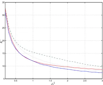
As a final comparison the results of all proposed condi-tions are shown together in Figure 12 forφ2_{= 0. In the}

dotted solid line (blue) it is shown the result of Theo-rem 1 the more conservative among they. This is justi-fied since no numerical tools are employed in Theorem 1 and only the upper bounds of the time-derivatives are considered. In dashed line (green) appears the result ob-tained with Theorem 6, the least conservative. The ex-planation for this is the opposite for the performance of Theorem 1, since in Theorem 6 numerical tools are em-ployed and the time-derivative informations are included in a less conservative manner, relying in the convexity of the polytopes (7). Theorem 3 against Theorem 4 there is no clear winner. For low and intermediate values of

φ1_{Theorem 4, signed with dotted line (black), is better.}

However asφ1_{raises Theorem 3 represented by solid line}

(12)

0.5 1 1.5 2 2.5 3 5

10 15 20 25 30 35

φ1

k

⋆

Figure 12: Stability analysis depending on second

time-derivatives of the membership functions: solid dotted line (blue) Theorem 1; solid line (red) Theorem 3; dotted line (black) 4; dashed line (green) Theorem 6.

6 CONCLUSION

As this paper has shown, the use of more information regarding the time-varying feature of TS fuzzy system is beneficial for stability analysis. New LMI tests based on the information regarding the second time-derivative of the membership functions were devised which improve stability analysis in comparison with standard parame-terized Lyapunov functions. Some conditions proposed in the recent literature can be viewed as particular cases. By resorting to a numerical tool capable to decouple sys-tems and function matrices improved conditions were obtained with respect to the conference version of this paper keeping computational effort in the same order of complexity.

7 ACKNOWLEDGEMENTS

The authors are grateful for the support of the agencies CNPq (Conselho Nacional de Desenvolvimento Cient´ı-fico e Tecnológico) and FAPEMIG (Funda¸cão de Am-paro à Pesquisa do Estado de Minas Gerais).

REFERENCES

Chesi, G., Garulli, A., Tesi, A. and Vicino, A. (2009). Homogeneous Polynomial Forms for Robustness Analysis of Uncertain Systems Homogeneous Poly-nomial Forms for Robustness Analysis of Uncertain

Systems, Vol. 390 ofLecture Notes in Control and

Information Sciences, Springer.

Feng, G. (2006). A survey on analysis and design of model-based fuzzy control systems,IEEE

Transac-tions on Fuzzy Systems14(5): 676 –697.

Feron, E., Apkarian, P. and Gahinet, P. (1996). Anal-ysis and synthesis of robust control systems via parameter-dependent Lyapunov functions, IEEE

Transactions on Automatic Control 41(7): 1041–

1046.

Fierro, R., Lewis, F. L. and Abdallah, C. T. (1996). Common, multiple and parametric Lyapunov func-tions for a class of hybrid dynamical systems, Pro-ceedings of the 4th IEEE Mediterranean

Sympo-sium of New Directions in Control and Automation,

Krete, Greece, pp. 77–82.

Gahinet, P., Apkarian, P. and Chilali, M. (1996). Affine parameter-dependent Lyapunov functions and real parametric uncertainty,IEEE Transactions on

Au-tomatic Control41(3): 436–442.

Geromel, J. C. and Colaneri, P. (2006). Robust stabil-ity of time varying polytopic systems, Systems &

Control Letters55(1): 81 – 85.

Haddad, W. M. and Chellaboina, V. (2008). Nonlin-ear Dynamical Systems and Control: a

Lyapunov-Based Approach, Princeton University Press.

Jadbabaie, A. (1999). A reduction in conservatism in stability and L2 gain analysis of Takagi-Sugeno

fuzzy systems,Proceedings of the 14th IFAC World

Congress, Beijing, China.

Lara, C., Flores, J. J. and Calderon, F. (2009). On the hyperbox – hyperplane intersection problem,

IN-FOCOMP - Journal of Computer Science8(4): 21–

27.

Montagner, V. F., Oliveira, R. C. L. F. and Peres, P. L. D. (2009). Convergent LMI relaxations for quadratic stabilizability andH∞control of Takagi– Sugeno fuzzy systems,IEEE Transactions on Fuzzy

Systems17(4): 863–873.

Mozelli, L. A. and Palhares, R. M. (2010). An´alise de es-tabilidade de sistemas fuzzy TS via LMI: Metodolo-gia baseada em uma nova fun¸c˜ao de Lyapunov fuzzy,Anais do XVIII Congresso Brasileiro de

Au-tom´atica - CBA’10, Bonito, MS, pp. 462–467.

Mozelli, L. A., Palhares, R. M. and Avellar, G. S. C. (2009). A systematic approach to improve multi-ple Lyapunov function stability and stabilization conditions for fuzzy systems,Information Sciences

(13)

Mozelli, L. A., Palhares, R. M., Avellar, G. S. C. and dos Santos, R. F. (2010). Condi¸cões LMIs alter-nativas para sistemas Takagi-Sugeno via fun¸cão de Lyapunov fuzzy, SBA: Controle & Automa¸cão

21(1): 96–107.

Mozelli, L. A., Palhares, R. M. and Mendes, E. M. A. M. (2010). Equivalent techniques, extra com-parisons, and less conservative control design for TS fuzzy systems, IET Control Theory &

Applica-tions4(12): 2813–2822.

Mozelli, L. A., Palhares, R. M., Souza, F. O. and Mendes, E. M. A. M. (2009). Reducing conserva-tiveness in recent stability conditions of TS fuzzy systems,Automatica45(6): 1580–1583.

Ohtake, H., Tanaka, K. and Wang, H. O. (2001). Fuzzy modeling via sector nonlinearity concept, Proceed-ings of the 20th International Conference of the North American Fuzzy Information Processing

So-ciety, Vol. 1, pp. 127 –132.

Oliveira, R. C. L. F., de Oliveira, M. C. and Peres, P. L. D. (2009). Special time-varying Lyapunov func-tion for robust stability analysis of linear parameter varying systems with bounded parameter variation,

IET Control Theory & Applications 3(10): 1448 –

1461.

Rhee, B.-J. and Won, S. (2006). A new fuzzy Lya-punov function approach for a Takagi-Sugeno fuzzy control system design, Fuzzy Sets and Systems

157(9): 1211 – 1228.

Sala, A. (2009). On the conservativeness of fuzzy and fuzzy-polynomial control of nonlinear systems,

An-nual Reviews in Control33(1): 48 – 58.

Takagi, T. and Sugeno, M. (1985). Fuzzy identifica-tion of systems and its applicaidentifica-tion to modeling and control,IEEE Transactions on Systems, Man, and

CyberneticsSMC-15(1): 116–132.

Tanaka, K., Hori, T. and Wang, H. O. (2003). A multi-ple Lyapunov function approach to stabilization of fuzzy control systems,IEEE Transactions on Fuzzy

Systems11(4): 582 – 589.

Tanaka, K. and Wang, H. O. (2001). Fuzzy Control Systems Design and Analysis: a Matrix Inequality

Approach, John Wiley & Sons.

Tanaka, K., Yoshida, H., Ohtake, H. and Wang, H. O. (2009). A sum-of-squares approach to modeling and control of nonlinear dynamical systems with poly-nomial fuzzy systems,IEEE Transactions on Fuzzy

Systems17(4): 911 –922.

Tanscheit, R., Gomide, F. and Teixeira, M. C. M. (2007). Modelagem e controle nebuloso, in L. A. Aguirre (ed.), Enciclop´edia de Autom´atica:

Cont-role & Automa¸c˜ao, Vol. 3, Blucher.

Teixeira, M. C. M., Assun¸c˜ao, E. and Avellar, R. G. (2003). On relaxed LMI-based designs for fuzzy regulators and fuzzy observers,IEEE Transactions

on Fuzzy Systems11(5): 613 – 623.

Teixeira, M. C. M. and Assun¸cão, E. (2007). Exten-sões para sistemas não-lineares, in L. A. Aguirre (ed.),Enciclopédia de Automática: Controle &