Projection of the Russian economic development in the framework of the optimal control model by investments in fixed assets

(1)

References

Information about the authors

JEL codes: C61, C62, C53, C02 А. М. Tarasyev, А. А. Usova, Yu. V. Shmotina

PROJECTION OF THE RUSSIAN ECONOMIC DEVELOPMENT

IN THE FRAMEWORK OF THE OPTIMAL CONTROL MODEL

BY INVESTMENTS IN FIXED ASSETS

1

In this paper, we develop an economic growth model taking into account two factors of production: ixed capital and labor force, to study the dynamics of GDP growth. The dependence of the output of these factors is described by a production function of the exponential type. Within the framework of the optimal control theory, the optimization problem for investment levels is being solved to maximize the integral index of con

(2)

Introduction

This paper is devoted to analysis of the eco -nomic growth model based on methods of the optimal control theory with a view to construct the optimal investment strategies. The consid -ered model in its design combines classical con -structions of the economic growth theory [1], and advanced methods of analysis of the opti -mal control theory [2], in particular, generali -zations of Pontryagin’s maximum principle for problems with ininite planning horizon [3-11]. is Investments in ixed assets serve as control pa -rameter and provide the output growth through the production function. In the balance equation the output is redistributed between consumption and investment, and this provides the model clos -edness in terms of control investment parameters. In this statement, the maximized characteristics is consumption, as in all classical models of inancial investments [12], for example, in the Fisher sta -tionary model and the Sharpe capital asset pricing model (CAPM) [13-14].

Application of the Pontryagin maximum prin -ciple in the model of economic growth gener -ates the Hamiltonian system of differential equa -tions, whose stationary points can be used to de -scribe the equilibrium trajectories of an economy, and whose trajectories — to build prognostic esti -mates of economic development. It is important to emphasize that the main element of the solution is the optimal programming control which can be interpreted as an optimal investment plan. We de -velop high accuracy algorithms for constructing optimal investment plans as trajectories of the Hamiltonian systems.

The paper is organized as follows. The pattern of the economic growth model is given the opti -mal control problem is posed for investments in ixed assets. Qualitative analysis of solutions is provided within Pontryagin’s maximum prin -ciple, stationary points are constructed for the Hamiltonian system generating economy equi -libria and stationary optimal investment plans. In conclusion, the model parameters are set to the real data in the framework of the econometric

analysis of the production function, which com -plements the study of the properties of the model Hamiltonian systems. A comparative analysis of the prognostic model trajectories and real time series is fulilled on the basis of the Russian mac -roeconomic data. Basic trends of model trajecto -ries are identiied and the key differences between these trends are indicated against the growth tra -jectories trends of developed economies.

Model of economic growth and the problem of optimal investment control

The basis of the model in the production block is presented by the production function, which is considered in the dynamic process of economic development. The main variables of the model are levels of capital K(t) and labor L(t) at time t, and the production output Y(t), which is given by the expo -nential production function of the Cobb-Douglas type [12]:

(

( ) ( )

)

( )

1

( )

,

( ) F K t L t aK t L t .

Y t ₌ ₌ α -α

Here a positive parameter α corresponds to the output which is provided by production fac -tors unaccounted in the model — Total Factor Productivity (TFP), and a nonnegative parameter α (0 <α< 1) is the elasticity coeficient.

Using the property of the positive homogene -ity of the irst order1 for the production function,

one can make transition to relative variables: cap -ital k t

( )

=K t

( ) ( )

/L t and GDP y t

( )

=Y t

( ) ( )

/L t

per one worker (per capita)

( )

_{( )}

( )

(

( ) ( )

_{( )}

)

( )

α

( )

= = =

 

= _ _= =

 

,

,1 ,

F K t L t Y t

y t

L t L t K t

F f k t ak t

L t (1)

where the function y t

( )

= f k t

( )

deines the la -bor productivity as a function of the capital-la-bor ratio.

Let us denote by symbols C(t) and I(t) consump -tion and investments in ixed assets at time t, re -spectively. Under assumption of the closedness of

1_{he property of the positive homogeneity of the irst order is} deined as follows ∀ν > 0 F

(

ν ν = νK L,

)

F K L

(

, .

)

sumption. We study the qualitative properties of optimal trajectories as solutions of the Hamiltonian systems arising in Pontryagin’s maximum principle. The sensitivity analysis of the equilibrium solutions of the eco -nomic system is implemented with respect to the elasticity coeficients of the production function, the depre -ciation rate of the capital, and the discount factor, and growth trends are indicated. The econometric analy -sis of the model parameters is provided basing on real data for the Russian economy. In accordance with the results of the regression analysis, the projection of economic development is constructed in conditions of the applicability of the economic growth model.

(3)

an economic system, one should require the bal -ance relation in each time period

( )

( ) ( )

( ) ( ) ( )

( )

_{( )}

( )

(

1

( )

)

,

Y t C t I t C t u t Y t C t

c t y t u t L t

= + = + ⇒

⇒ = =

-where the function u(t) corresponds to the share of GDP invested in ixed assets, i.e. I t

( ) ( ) ( )

=u t Y t .

The relative value of c(t) is the level of consump -tion per one worker. One can derive restric-tions on the investment levels from the balance equation,

( ) ( )

(

( )

)

( )

0 1 ,

0 1.

c t y t u t y t u t u

≤ = - <

≤ ≤ < (2) This version of the model assumes that the growth of the capital stock K(t) is subject to the dynamics introduced by Solow [1]

( ) ( ) ( )

( )

0

, 0 ,

,

, 0

K t u t Y t K t K K L t

n L L L t

= -µ =

= =



where a positive coeficient µ is the depreciation rate of capital, and a constant value of n stands for the growth rate of the labor force L(t).

Passing to the relative values in the last rela -tions, we obtain the following dynamics for k(t)

( ) ( )

( )

( ) ( )

0 0

0

, 0 K

k t u t f k t k t k k

L

= -δ = =

 ₍₃₎

where the parameter δ = µ +n is the degree of cap -ital dilution due to its depreciation and increase in the labor force.

Let us consider the problem of optimal control of investment in which the objective functional is given by the integral of the logarithmic index of consumption, discounted on the ininite time interval:

( )

(

( )

)

(

)

+∞ -ρ +∞ -ρ ⋅ = = = +

-∫

∫

0 0 ln

ln ln 1 ,

t

J e c t dt

e f k t u t dt (4)

where ρ is the discount factor.

Let us note that in the utility theory, the log -arithmic function describes the relative increase (in our case — the relative consumption) per unit of time. Under conditions of uncertainty the log -arithmic function speciies the constant relative risk aversion.

Problem. It is necessary to construct such an investment strategy (k(t), u(t)) that satisies the constraints (2) and maximizes the objective func

-tional (4) on trajectories of the dynamical system (3).

Analysis of the optimal control problem within the framework of Pontryagin’s

maximum principle

The posed problem of optimal control is sub -ject to a modiication of Pontryagin’s maximum principle for the ininite time period [3-11].

Let us construct the stationary Hamiltonian function of the control problem which due to the dynamics (3) and the objective functional of the control process (4) has the following form with the conjugate variable ψ

(

, ,

)

ln

( )

ln 1

(

)

(

( )

)

.

H k ψu = f k + - + ψu uf k -δk (5) Let us calculate the control u0, delivering max -imum to the Hamiltonian H (5)

(

)

_{( )}

( )

∂ ψ

= - + ψ ⇒

∂

-

 _< _{ψ ≤}

 

⇒ ψ =_ - ≤ ψ ≤

-ψ

 

 ψ ≥

-

0

, , 1

1

0, 0 1,

1 1

, 1 , 1 ,

1

, .

1

H k u

f k

u u

f k

u k f k

u f k

u (6)

The maximum control 0

( )

_,

u k ψ (6) divides the domain of variables

( )

k, ψ into three domains with the different structure of the Hamiltonian dynamics deined by relations

( )

(

( ) ( )

(

( ) ( )

)

( ) ( )

(

)

( )

∂ ψ ψ

= =

∂ψ

= ψ -δ

0

, , ,

, ,

H k t t u k t t dk t

dt

u k t t f k t k t (7)

( )

_{( )}

(

( ) ( )

(

( ) ( )

)

( )

_{( )}

( )

(

( ) ( )

)

( )

)

∂ ψ ψ

ψ

= ρψ - =

∂

= ρψ - - ψ ψ - δ

0

'

0 '

, , ,

, .

H k t t u k t t d t

t

dt k

f k

t t u k t t f k t f k

Let us consider the Hamiltonian system (7) for three different control modes.

Zero control mode

The domain of the zero control mode

( )

0 _, ₀

u k ψ = is determined by the relations

( )

0< f k ψ ≤1. The Hamiltonian system with this control can be written as

( )

_{( )}

( ) ( ) ( ) ( )

_{( )}

= -δ

ψ

= ρ + δ ψ

-' , . dk t k t dt

d t f k

t

(4)

Passing to the normalized dynamics, we obtain the system of differential equations in variables

( )

k z, where z k= ψ

( )

_{( )}

( )

_{( )}

( )

= -δ

= ρ - = ρ - α

, ' . dk t k t dt

dz t f k

z t k z t

dt f k (8)

As one can see from the structure of the sys -tem (8), its solution declines exponentially to zero at the rate of depreciation of ixed assets δ with re -spect to the phase component of capital k(t). Thus, the lack of the investment component leads to re -duction of the capital stock up to the zero level.

Transient control mode

The transient control mode is characterized by a non-zero share of output invested in ixed assets that is calculated by the formula

( )

_{( )}

0 1

, 1 1 k ,

u k z k

f k f k z

ψ = - = - = ψ

ψ

and meets restrictions: ≤

( )

≤ -1

1 .

1

f k z

k u

The Hamiltonian system in the variable control mode has the following structure

( )

_{( )}

( )

(

)

( )

_{( )}

( )

   

= - -δ

 

 

 

 

= ρ - + - =

 

 

 

 

= ρ + - α

-    ' 1 , 1 1 1.

f k t dk t

k t dt k t z t

f k t dz t

f k t z t

dt k t

f k t z t

k t (9)

Saturated control mode

The saturated control mode is presented by the highest possible level of investments in ixed as -sets _{u k}0

( )

_,_{ψ =}_u

, and is constrained by the limi -tations f k

( )

ψ ≥1 / (1 )-u . Under these conditions, the Hamiltonian system (7) in the variable (k, z) has the following form

( )

_{( )}

( )

(

)

( )

    = -δ        

= ρ - +

- 

 

 

 

- = ρ + - α - α

    , ' ' 1 .

f k t dk t

u k t

dt k t

f k t dz t

uf k t u z t

dt k t

f k t k t f k t

u z t

k t

f k t (10)

In the last formulas, we use the following prop -erties of the Cobb-Douglas production function of the exponential type:

( )

_{= α} α- _{= α} α _{= α}

( )

_⇒

( )

_{( )}

_{= α}

'

1

' ak f k f k k .

f k a k

k k f k

Equilibrium of economy in the maximum principle

Stationary levels of the Hamiltonian system (7) determine the equilibrium positions of the economic system. In order to ind these levels we equate the right sides of the Hamiltonian systems (8)–(10) to zero and solve the system of non-lin -ear algebraic equations in variables (k, z) under conditions k>0, z>0, ψ >0.

Evidently, the Hamiltonian system (8) for the zero control regimes does not have stationary lev -els satisfying the constraints k>0, z>0. However, in domains of the transient and saturated control regimes steady states exist and their coordinates are determined analytically through the model parameters.

Proposition. The equilibrium points in the do -main of the transient control and the do-main of the saturated control are given by the formulas

(

)

( )

(

)

-α -α α 

 α  αδ

_ _ ₌ _<

 δ + ρ_ _ δ + ρ  =    _ _ = δ    α = =

ρ + - α δ

= 1 1 * * 1 1 * * * * * * * , , , , , , 1 1 .

a _u _u

k

ua _u _u

z y a k

c y u

Proof. 1) Let us calculate the coordinates of the equilibrium point in the transient control re -gime. It is necessary to equate the right sides of the Hamiltonian system (9) to zero

( )

(

) ( )

(

)

(

)

( )

-α - -δ = ⇒ = δ +

 

ρ + - α - = ⇒

 

 

  

⇒ ρ + - α δ +_ _ __ =

 

α ρ + δ

= ⇒ = ⇒

α ρ + - α δ

 α 

⇒ _{= } _

δ + ρ

  * * * * * * 1 1 * 1 1

0 ,

1 1 0

1 1 1, 1 . f k f k

k z k z

(5)

Let us calculate the control value correspond -ing to the equilibrium level

( )

(

)

*

* *

1

1 k 1 1

u

f k z

α ρ + - α δ _αδ

= - = - = <

δ + ρ

ρ + δ α .

The equilibrium point is located in the domain of the transient control if _u* _<_u

. Therefore, if the model parameters meet the constraints

u

αδ _< δ + ρ , the equilibrium point * * *

( , , )k z u is attained in the domain of the transient control.

2) Let us calculate the coordinates of the equi -librium point in the domain of the saturated con -trol when u t

( )

=u. In order to do this, one should resolve the system of nonlinear algebraic equa -tions determined by the right hand sides of the Hamiltonian dynamics (10)

( )

(

) ( )

(

)

(

)

(

)

-α

δ  

-δ = ⇒ = ⇒ _{=  }

δ  

 

ρ + - α - α = ⇒

 

 

⇒ ρ + - α δ = α ⇒ α

⇒ =

ρ + - α δ

1 * 1 * * * *

0

1 0 1 . , 1 f k

f k _au

u k

k k u

f k

u z

k z

z

The equilibrium control coincides with the maximum possible investment level into capital, i.e. *

u =u.

The equilibrium level of the output is calcu -lated by the formula (1)

( ) ( )

* * *

y =f k =a k α.

The equilibrium level of consumption, ex -pressed through the balance equation, is given by the following relation

(

)

* * *

1

c = -u y. Proposition is proved.

Analytical expressions for the values of in -vestment u*, capital k*, output volume y* and con -sumption c* allow to analyze the sensitivity of the stationary equilibrium state in terms of the elasticity coeficients for the model parameters α, δ, ρ. Signs of elasticity coeficient indicate of the growth and decrease trends. Their absolute values indicate the change rates in percentage terms.

Calculation of the logarithmic values of deriv -atives of investments k* at the equilibrium point provides the following values for the elasticity co -eficients with respect to the model parameters

α δ

ρ

α ∂ δ ∂ ρ

e = = e = = <

∂α ∂δ δ + ρ

ρ ∂ ρ

e = = - <

∂ρ δ + ρ

* * , * , * * , * 1, 1, 0. u u u u u u u u u

Coeficients of elasticity show that the equi -librium investments in capital u* increases to -gether with the growing elasticity α of the pro -duction function and the growing capital depre -ciation rate δ, and it decreases when the discount factor ρincreases.

Elasticity coeficients for the equilibrium out -put of production y* with the respect to the model parameters have the following expressions

α

δ

ρ

α ∂ α  α

e = = _ + _

∂α - α_ - α_

δ ∂ α δ

e = = - ⋅ <

∂δ - α δ + ρ

ρ ∂ α ρ

e = = - ⋅ <

∂ρ - α δ + ρ * , * * , * * , * ln 1 , 1 1 0, 1 0. 1 y y y y y y y y y

Negative signs of the elasticity of the equilib -rium production level y* with respect to changes in the capital depreciation rate δ and the discount factor ρ indicate the decline trend. As for the sign of the elasticity of the equilibrium production level y* with respect to changes in the elasticity α of the production function, it is worth to note that small values of the elasticity α make it negative and large values of the elasticity of a make it pos -itive. It means that here both decreasing and in -creasing trends can be obtained.

If the equilibrium level of capital satisies the constraint u*<u, then one can observe the decline trend over time of the optimal investments to the level of u*. Otherwise, the maximum level of in -vestments is the best possible value on the en -tire time interval until the time of stabilization of the dynamical system. In all development scenar -ios the pattern of optimal solutions is conigured in the expressed S-shape, which is ensured by the presence of the parameter constraints u on invest -ments u(t). In addition, one can note that the op -timal trajectories have a tendency to the satura -tion growth.

An algorithm for constructing optimal model trajectories

(6)

-tions for the adjoint variable z(t) are given on the right side of the time interval. In this connection, a two-step integration procedure is developed.

1. The irst step. The system is integrated by the Runge-Kutta method in the reverse time from the equilibrium point in the direction of the ei -genvector of the Jacobian matrix corresponding to the negative eigenvalue. Integration is imple -mented until the integrated trajectory reaches the initial point of the phase variable.

2. The second step. Integration is performed in the direct timeline from the initial point. During this process, the components of the optimal model trajectory are reconstructed including the optimal investment plan u0(t).

It is important to emphasize that the two-step integration process provides a highly accurate al -gorithm for constructing optimal model trajec -tory with the order higher than the time step of integration.

Econometric analysis of the parameters of the production function

It is worth to emphasize that construction of prognostic model trajectories and econometric analysis of the production function and other pa -rameters of the model are complementary tasks, but they are carried out in separate blocks with different functions. The econometric analysis is based on the classical methods of econometrics [15-16] and is used to identify the model parame -ters, in particular, the elasticity coeficients of the production function and setting the total factor productivity. The numerical algorithms, after sub -stituting parameters identiied in the econometric analysis, work ofline producing optimal trajectory of endogenous growth. Another important issue is that the simulation procedure does not attempt to construct the trajectories of the best approxima -tion of the real time series. It builds namely the optimal investment plan and the optimal trajec -tory of economic growth. If the optimal model tra -jectory is close to the real data of economic de -velopment, then this fact indicates the optimal economic growth of the analyzed economic sys -tem in the sense of the integral consumption in -dex. In the case of deviations of the optimal model trajectory from the data in the “upper” or “lower” direction, it is reasonable to discuss a phenome -non of underinvestment or overinvestment in the economic system. In this context, the model con -structs the optimal investment plan that indi -cates imbalances with the real data. Therefore, the model trajectories could be called optimal prog -nostic trajectories to distinguish them from fore -casts of econometric models.

The calibration procedure for the production function (1) is fulilled on the basis of the statisti -cal data [17-18] of the Russian economy in the pe -riod from 1990 to 2011 using the paired-regres -sion model

i i

w = α + βx ,

where wi = ln , y xi i =ln , ki β =ln , a i=1,22.

Estimates of the paired-regression model pa -rameters are calculated by the least squares method:

(

)

( )

α = = β = - α = ⇒

σ

⇒ = 2

0,836

cov , _ˆ

ˆ 0,836, ˆ 0,249

ˆ

1,283 .

w x

w x x

y k

Curves on Figure 1 show the real data (in black) and the trajectory constructed using the regres -sion model (in grey).

To assess the quality of the regression model the coeficient of determination 2

0,909 R = is cal -culated whose value indicates a good “matching” with the real data. The results of testing the signif -icance hypothesis of the regression model suggest that the ixed capital has a signiicant impact on

Fig. 1. Comparison of real data and predictive values of GDP (black) on the simple regression model (grey)

(7)

the level of country’s GDP, and this is conirmed by the following calculation:

1. Evaluation of the error variance:

2 1 2

0,03

2 i

s e

N

= =

-

∑

.

2. Evaluation of the variance for the elasticity coeficient, σ α2

( )

ˆ

ˆ :

( )

₍

₎

σ α = =

-∑

2 2

ˆ 0,0032.

ˆ

i

s x x

3. The observed value of the Student’s statis -tics for N- =2 20 degrees of freedom:

( )

α

= =

σ α ˆ

14,86.

ˆ ˆ

t

4. The critical value at the level of the statisti -cal reliability, γ =95%:

(

)

1 2

2 2,086

k k

t =t-γ N- = ⇒ >t t.

Prognostic model trajectories and comparison with econometric time series

Returning to the described model of economic growth, let us construct its solutions numerically [4-11], and compare these solutions with real data. To construct the prognostic trajectories we use re -sults of the regression analysis for the production function, as well as data on the Russian economy for the period from 1990 till 2011 [17-18]. The es -timated indices of economic development are cal -culated at the levels:

= = = =

* _5.97, * _5.74,* _0.443,* _3.195,

k y u c

taking into account the economic indicators [17-18] given in the list.

1. The level of depreciation of ixed assets ac -cording to Rosstat [18] is estimated as 42% in av -erage, thus, the parameter µ is equal to 0.42.

2. The growth rate of the labor force n is esti -mated at the level of 0.004 in the period from 1990 to 2011.

3. The discount factor ρ according to the data [18] of the Central Bank of the Russian Federation on the reinancing rate is ixed at the level of 0.08.

4. The level of investments in ixed assets, ac -cording to Rosstat [18] has a clearly expressed in -creasing trend (see Figure 2). Therefore, to con -struct the prognostic trajectory the maximum level of investments u is chosen at a suficiently high level of 44.3%. However, even the investment limit of 44.3% does not meet the inequality

αδ ₌ _< δ + ρ 0,703 .u

This fact indicates that the investment trajec -tory does not decrease during the forecast period.

And selection of a smaller value u for the maxi -mum investment level leads to the economy with practically zero growth.

The model shows that the optimal level of in -vestments in the Russian economy in the current period is implemented on the upper level of con -straints. Let us note that a series of experiments, with different restrictions on the maximum level of investments have been conducted and the out -come remained the same: the optimal level of in -vestments is realized at the upper limit. This means that investments in ixed assets in the econ -omy are insuficient and require increase even for the upper threshold. For comparison, in modeling developed economies such as economies of the US [8-11], Japan [4-7], and the UK [4-5], one can ob -serve a qualitatively different picture. Namely, the model investment plans have the tendency to de -crease to the stationary equilibrium level u* < u, which indicates the situation of over-investment in ixed assets in these countries.

Fig. 3. Prognostic growth rates (black) of ixed capital per cap-ita of working population in comparison with real data (grey)

(8)

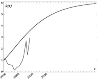
On Figures 3 and 4 the prognostic model tra -jectories of the Russian economic development with projections to 2050 are presented in compar -ison with the real data.

The presented plots clearly indicate that in the 90th years there is a rapid reduction in pro -duction and investments in ixed assets, which is expressed in sharp drops of real statistical trends. At the same time, the prognostic model trajecto -ries clearly demonstrate a growing trend, since the model is inherently focused on the search for such an investment strategy that leads the economy to the growth domain. The investments growth is positively relected in the statistics of the dy -namics, as one can see on the presented graphs. Namely, starting from 2000 clear growth trends are shaped for the main considered factors (ex -cepting the recession of 2008), and by the end of the analyzed period the actual data almost reach the model trends.

It should be noted that the comparative anal -ysis of modeling results for the macroeconomic data on countries’ economies in different groups shows that the values of the identiied model pa -rameters in these groups are qualitatively differ -ent by clusters. These differences affect, irst of all, the dynamics of investment plans. In econo -mies of developed countries, one can observe the

decline trend in investments (in percentage) with higher initial levels to lower stationary equilib -rium levels. For economies of developing countries there is a bifurcation and qualitatively different trends are observed when the value of the equilib -rium investments is very high in comparison with the actual current levels. This leads to the situa -tion when the model optimal investments should reach the highest possible limit values.

Conclusion

The paper deals with analysis of the model of economic growth within the framework of the op -timal control theory. The problem of optimizing the investment levels is considered, the solutions are constructed within the Pontryagin maximum principle, and analysis of trends is fulilled for the optimal model trajectories. Identiication of pa -rameters and analysis of signiicance of the re -gression model are implemented for the produc -tion func-tion. Basing on algorithms for numerical construction of optimal prognostic trajectories, the model growth trends are identiied; equilib -rium points of major economic indicators are cal -culated and compared with real statistical data of the Russian economy. Major differences are in -dicated between the identiied trends and the growth trajectories in developed economies.

he study is supported by the grant of the Russian Scientiic Fund (project No. 14-18-00574 “Information and analytical “Anti-crisis” system: diagnostics of regions, threat assessments, and scenario forecasting for the purpose of maintaining and strengthening of economic security and improve welfare of Russia”).

References

1. Solow, R. M. (1970). Growth heory: An Exposition. NY, Oxford Univ. Press, 190.

2. Pontryagin, L. S., Boltyanskiy, V. G., Gamkrelidze, R. V. & Mishchenko, E. F. (1962). Matematicheskaya teoriya optimalnykh [he Mathematical heory of Optimal Processes], Interscience, New York, 363.

3. Aseyev, S. M., Kryazhimskiy, A. V (2007). he Pontryagin Maximum Principle and Optimal Economic Growth Problems. Proceedings of the Steklov Institute of Mathematics. Pleiades Publishing, Vol. 257, 1, 5-271.

4. Krasovskiy, A. & Tarasyev, A. (2008). Conjugation of Hamiltonian Systems in Optimal Control Problems. Proceedings of the 17th IFAC World Congress, 17, 1, COEX, Korea, South, 7784-7789. DOI: 10.3182/20080706-5-KR-1001.01316.

5. Krasovskiy, A., Kryazhimskiy, A. & Tarasyev, A. (2008). Optimal Control Design in Models of Economic Growth. Evolutionary Methods for Design, Optimization and Control (P. Neittaanmäki, J. Périaux and T. Tuovinen, Eds.), CIMNE, Barcelona, Spain, 70-75. 6. Krasovskiy, A. A. & Tarasyev, A. M. (2008). Svoystva gamiltonovykh system v printsipe maksiuma Pontryagina dlya zadach ekonomicheskogo rosta [Properties of Hamiltonian Systems in the Pontryagin Maximum Principle for Economic Growth]. Trudy matematicheskogo institute im. Steklova V.A. [Proceedings of the Steklov Mathematical Institute], 262, 127-145.

7. Krasovskiy, A. A. & Tarasyev, A. M. (2009). Postroyenie nelineynykh regulyatorov v modelyakh ekonomicheskogo rosta [Construction of Nonlinear Stabilizers in Economic Growth Models]. Trudy Instituta matematiki i mekhaniki [Proceedings of the Institute of Mathematics and Mechanics], Yekaterinburg: Ural Branch of RAS, Vol. 15, 3, 127-138.

8. Tarasyev, A. M. & Usova, A. A. (2011). he Value Function as a Solution of Hamiltonian Systems in Linear Optimal Control Problems with Ininite Horizon. Proceedings of the 18th IFAC World Congress, Milan, Vol. 18, Part 1, 2927-2933.

9. Tarasyev, A. M. & Usova, A. A. (2010). Postroyenie regulyatora dlya gamiltonovoy sistemy dvukhsektornoy modeli eko-nomicheskogo rosta [Developmet of a Stabilizer for the Hamiltonian system of a Two-Sector Model of Economic Growth]. Trudy matematicheskogo instituta im. V. A. Steklova [Proceedings of the Steklov Mathematical Institute], 271, 278-298.

10. Tarasyev, A. M. & Usova, A .A. (2012). Stabilizatsiya gamiltonovoy sistemy dlya postroyeniya optimalnykh trayektoriy [Stabilization of Hamiltonian systems for Constructing Optimal Trajectories]. Trudy matematicheskogo instituta [Proceedings of the Steklov Mathematical Institute], 277, 257-274.

(9)

12. Intriligator, M. (1971). Matematicheskie metody optimizatsii i ekonomicheskaya teoriya [Mathematical Optimization and Economic heory]. Prentice-Hall, N.Y., 553.

13. Krushvits, L.(1995). Finansirovanie i invistitsii [Finanzierung und Investition] . Walter De Gruyter Inc., Berlin, 400. 14. Sharpe, W. F., Alexander, G. J. & Bailey J. V. (1999). Investitsii [Investments]. Sixth Edition. Prentice-Hall, N.Y., 965. 15. Ayvazyan, S. A. (2010). Metody ekonometriki [Methods in Econometrics]. Moscow: INFRA-M, 512.

16. Magnus, Y. R., Katyshev, P. K. & Peresetskiy, A. A. (2007). Ekonometrika [Econometrics]. Moscow: DELO, 580. 17. OECD Statistics. Available at: http://stats.oecd.org, 2012.

18. Federalnaya sluzhba gosudarstvennoy statistiki RF (FSGS RF) [Federal State Statistics Service (Rosstat)]. Available at: http:// www.gks.ru/wps/wcm/connect/rosstat_main/rosstat/ru/statistics.

Information about the authors

Tarasyev Alexander Mikhajlovich (Yekaterinburg, Russia) — Dr. Phys.–Math. Sci., Head of Sector, the Institute of Mathematics and Mechanics named ater N. N. Krasovskii of the Ural Branch of the Russian Academy of Sciences; Research Scholar, International Institute for Applied Systems Analysis (IIASA) (16, S. Kovalevskaya str., Yekaterinburg, 620990, Russia, e-mail: [email protected]).

Usova Anastasy Aleksandrovna (Yekaterinburg, Russia) — PhD in Phys.-Math. Sci., Research Scholar, the Institute of Mathematics and Mechanics named ater N.N. Krasovskii of the Ural Branch of the Russian Academy of Sciences (16, S. Kovalevskaya str., Yekaterinburg, 620990, Russia, e-mail: [email protected]).

Shmotina Yulia Valer’evna (Yekaterinburg, Russia) — student, the Institute of Mathematics and Computer Science, the Ural Federal University named ater the irst President of Russia B.N. Yeltsin (19, Mira str., Yekaterinburg, 620002, Russia, e-mail: [email protected]).

A. A. Krasovskii, N. V. Khabarov, M. Obersteiner

IMPACTS OF THE FAIRLY PRICED REDD BASED CO OFFSET OPTIONS

ON THE ELECTRICITY PRODUCERS AND CONSUMERS

This paper deals with the modeling of two sectors of a regional economy: electricity and forestry. We show that CO₂ price will impact not only the proits of the CO₂ emitting electricity producer (decrease), but also the electricity prices for the consumer (increase), and, hence, some inancial instruments might be implemented today in order to be prepared for the uncertain CO₂ prices in the future. We elaborate inancial instrument based on the Reduced Emissions from Deforestation and Degradation (REDD+) mechanism. We model op timal behavior of forest owner and electricity producer under uncertainty and determine equilibrium fair prices of REDD-based-options.

Introduction

This research is focused on developing inan cial instruments supporting activities within the framework of the Reducing Emissions from Deforestation and Forest Degradation Plus (REDD+) program. The basic idea of the program is that REDD+ would provide payments to juris dictions (countries, states, or provinces) that re duce forest emissions below agreed-upon bench mark levels . In a recent review [1] authors discuss the potential of REDD+ and show that there are many research needs and opportunities for ana