Radiative forcing and climate response to projected 21st century aerosol decreases

(1)

ACPD

15, 9293–9353, 2015

Climate response to aerosol decreases

D. M. Westervelt et al.

Title Page

Abstract Introduction

Conclusions References

Tables Figures

◭ ◮

Back Close

Full Screen / Esc

Printer-friendly Version Interactive Discussion

Discussion

P

a

per

|

Discussion

P

a

per

|

Discussion

P

a

per

|

Discussion

P

a

per

|

Atmos. Chem. Phys. Discuss., 15, 9293–9353, 2015 www.atmos-chem-phys-discuss.net/15/9293/2015/ doi:10.5194/acpd-15-9293-2015

This discussion paper is/has been under review for the journal Atmospheric Chemistry and Physics (ACP). Please refer to the corresponding final paper in ACP if available.

Radiative forcing and climate response to

projected 21st century aerosol decreases

D. M. Westervelt1, L. W. Horowitz2, V. Naik3, and D. L. Mauzerall1,4

1

Program in Science, Technology, and Envrionmental Policy, Woodrow Wilson School of Public and International Affairs, Princeton University, Princeton, NJ, USA

2

Geophysical Fluid Dynamics Laboratory, National Oceanic and Atmospheric Admnistration, Princeton, NJ, USA

3

UCAR/NOAA Geophysical Fluid Dynamics Laboratory, Princeton, NJ, USA

4

Department of Civil and Environmental Engineering, Princeton University, Princeton, NJ, USA

Received: 25 February 2015 – Accepted: 13 March 2015 – Published: 27 March 2015

Correspondence to: D. M. Westervelt (danielmw@princeton.edu) and D. L. Mauzerall (mauzeral@princeton.edu)

(2)

ACPD

15, 9293–9353, 2015

Title Page

Tables Figures

◭ ◮

Back Close

Full Screen / Esc

Discussion

P

a

per

|

Discussion

P

a

per

|

Discussion

P

a

per

|

Discussion

P

a

per

|

Abstract

It is widely expected that global emissions of atmospheric aerosols and their precursors will decrease strongly throughout the remainder of the 21st century, due to emission reduction policies enacted to protect human health. For instance, global emissions of aerosols and their precursors are projected to decrease by as much as 80 % by the year

5

2100, according to the four Representative Concentration Pathway (RCP) scenarios. The removal of aerosols will cause unintended climate consequences, including an un-masking of global warming from long-lived greenhouse gases. We use the Geophysical Fluid Dynamics Laboratory Climate Model version 3 (GFDL CM3) to simulate future cli-mate over the 21st century with and without the aerosol emission changes projected by

10

each of the RCPs in order to isolate the radiative forcing and climate response resulting from the aerosol reductions. We find that the projected global radiative forcing and cli-mate response due to aerosol decreases do not vary significantly across the four RCPs by 2100, although there is some mid-century variation, especially in cloud droplet ef-fective radius, that closely follows the RCP emissions and energy consumption

projec-15

tions. Up to 1 W m−2_{of radiative forcing may be unmasked globally from 2005 to 2100} due to reductions in aerosol and precursor emissions, leading to average global tem-perature increases up to 1 K and global precipitation rate increases up to 0.09 mm d−1_. Regionally and locally, climate impacts can be much larger, with a 2.1 K warming pro-jected over China, Japan, and Korea due to the reduced aerosol emissions in RCP8.5,

20

as well as nearly a 0.2 mm d−1 _{precipitation increase, a 7 g m}−2 _{LWP decrease, and} a 2 µm increase in cloud droplet effective radius. Future aerosol decreases could be responsible for 30–40 % of total climate warming by 2100 in East Asia, even under the high greenhouse gas emissions scenario (RCP8.5). The expected unmasking of global warming caused by aerosol reductions will require more aggressive greenhouse gas

25

(3)

ACPD

15, 9293–9353, 2015

Title Page

Tables Figures

◭ ◮

Back Close

Full Screen / Esc

Discussion

P

a

per

|

Discussion

P

a

per

|

Discussion

P

a

per

|

Discussion

P

a

per

|

1 Introduction

The climate e_ffects of atmospheric aerosols represent one of the most uncertain as-pects of current and future climate forcing and response estimates (IPCC, 2013). Whereas the greenhouse gas warming influences on climate are relatively well un-derstood, significant questions remain regarding the magnitude, and in some cases,

5

even the sign (cooling or warming), of aerosol-climate interactions. Aerosol radiative forcing of climate can be split into two categories: the direct effect, in which atmo-spheric aerosols directly scatter or absorb incoming solar radiation; and the indirect effect, in which aerosols modify cloud properties which in turn affect the radiation bud-get. For a fixed amount of cloud water, a more polluted air mass will have smaller and

10

more numerous cloud droplets, leading to a larger surface area and a brighter cloud (Twomey, 1977). This is known as the cloud albedo effect. In addition, more aerosol pol-lution may also result in a longer cloud lifetime due to the tendency of smaller droplets to remain suspended in the atmosphere longer (Albrecht, 1989), although this cloud lifetime effect is not as well understood. Generally, both the direct and indirect effects

15

tend to exert a net negative radiative forcing on present-day climate, leading ultimately to a decrease in average global temperature, with the total aerosol e_ffective radiative forcing estimated to be −0.9 W m−2 (uncertainty range −1.9 to −0.1 W m−2) (Myhre

et al., 2013). This aerosol forcing has likely offset a significant portion of present-day CO₂and other greenhouse gas-induced climate forcing and subsequent global

warm-20

ing. Likewise, any changes in future anthropogenic aerosols will have implications for the overall net impact on climate. Here we evaluate the changes in global and re-gional aerosol burden, climate forcing, and climate response due to future decreases in aerosol and precursor emissions as projected by all of the Representative Concen-tration Pathways (RCPs). We build upon the work of Levy et al. (2013) to contrast the

25

(4)

ACPD

15, 9293–9353, 2015

Title Page

Tables Figures

◭ ◮

Back Close

Full Screen / Esc

Discussion

P

a

per

|

Discussion

P

a

per

|

Discussion

P

a

per

|

Discussion

P

a

per

|

Emissions of aerosols and their precursors have increased dramatically since the preindustrial era, due to increasing industrialization and global population. In 2012, air pollution, mostly in the form of atmospheric aerosols, was responsible for 7 million deaths (3.7 million from ambient air pollution, 3.3 million from indoor) worldwide (WHO, 2014). Due to e_fforts to reduce this enormous human health impact, aerosol and

pre-5

cursor emissions are expected to decline worldwide over the next several decades as governments enact and enforce stricter emission control policies. Emissions of sulfur dioxide (SO₂, a precursor to sulfate aerosol) have already declined about 50 % in North America and Western Europe and passed their peak in 2005 in China (Lamarque et al., 2010). In some developing countries, emissions are still rising but are expected to

be-10

gin to decline within the next few decades, as a consequence of increasing a_ffluence and more environmental regulation (van Vuuren et al., 2011a).

While clearly beneficial for human health, declining aerosol emissions will result in the unintended consequence of unmasking additional climate warming, due to the re-duction of the cooling e_ffects from anthropogenic aerosols such as sulfate and organic

15

carbon (OC). Thus, careful policy implementation is necessary in order to maximize reduction of unhealthy air pollution while also minimizing the unmasking of additional global warming. Some studies have pointed to reductions in black carbon as a possible approach to address this dilemma (Bond et al., 2013; Kopp and Mauzerall, 2010; Shin-dell et al., 2012a). Black carbon (BC) is an aerosol species that is a strong absorber

20

of incoming solar radiation in the troposphere and thus a climate-warming agent. It is also a major contributor to PM_2.5 and has an adverse effect on human health (Bond et al., 2013). Despite a clear human health benefit, questions remain whether its re-duction will be an e_ffective strategy for avoiding additional warming, due to its frequent co-emission with two strong cooling species, OC and sulfate (Chen et al., 2010;

Red-25

(5)

ACPD

15, 9293–9353, 2015

Title Page

Tables Figures

◭ ◮

Back Close

Full Screen / Esc

Discussion

P

a

per

|

Discussion

P

a

per

|

Discussion

P

a

per

|

Discussion

P

a

per

|

Aerosols also have strong impacts on precipitation, cloud cover, cloud droplet size and number, atmospheric circulation, and other climate parameters (Lohmann and Fe-ichter, 2005; Ming and Ramaswamy, 2009, 2011; Ming et al., 2011; Ramanathan et al., 2001; Rosenfeld et al., 2008; Stevens and Feingold, 2009). An increase in aerosol emissions tends to decrease precipitation rates, through macrophysical and

micro-5

physical processes: (1) less incoming solar radiation penetrates the troposphere and reaches the surface, resulting in less evaporation (Ramanathan et al., 2001) and (2) smaller and more abundant aerosols lead to smaller cloud droplets, which are less likely to convert to rain drops via coalescence on the local and regional scale (Radke et al., 1989; Rosenfeld, 2000). An exception to (1) is BC or other absorbing aerosols,

10

which may have opposing effects on precipitation through heating the atmosphere (causing stabilization and reduction in precipitation) and warming the surface (caus-ing an enhancement of precipitation) (M(caus-ing et al., 2010). However, the net e_ffect of increasing aerosol concentrations tends to be suppression of precipitation. Thus, the expected reduction of aerosol concentrations should increase rainfall rates globally.

15

Since aerosols serve as seeds for virtually all cloud formation in the atmosphere, de-creases in aerosols may also be expected to affect cloud cover, cloud liquid water path, and e_ffective cloud droplet radius.

To estimate future aerosol emissions and burden, radiative forcing, and climate re-sponse, we must rely on future projections or scenarios. The current state-of-the-art

20

emissions scenarios for global climate modeling are the Representative Concentration Pathways (RCP) (Lamarque et al., 2011; Masui et al., 2011; Riahi et al., 2011; van Ruijven et al., 2008; Thomson et al., 2011; van Vuuren et al., 2011a, b, 2012). The RCPs are different from previously developed scenarios in that they are initialized with radiative forcing beginning and endpoints (2005–2100). A consistent but non-unique

25

(6)

green-ACPD

15, 9293–9353, 2015

Title Page

Tables Figures

◭ ◮

Back Close

Full Screen / Esc

Discussion

P

a

per

|

Discussion

P

a

per

|

Discussion

P

a

per

|

Discussion

P

a

per

|

house gases and air pollutants, including emissions of three aerosol/precursor species: SO₂, OC, and BC. All RCPs assume an autonomous change in future air pollution con-trol policies in every world region, resulting in sharp decreases in regional and global emissions of SO₂, OC, and BC.

There have been several previous studies on the e_ffects of diminishing emissions of

5

aerosols and their precursors on aerosol burden, radiative forcing, and climate (Arneth et al., 2009; Bellouin et al., 2011; Chalmers et al., 2012; Gillett and Von Salzen, 2013; Kloster et al., 2009; Lamarque et al., 2011; Leibensperger et al., 2012; Makkonen et al., 2011; Menon et al., 2008; Rotstayn et al., 2013; Shindell et al., 2013; Smith and Bond, 2014; Takemura, 2012; Unger et al., 2009). These studies and their results are

10

summarized in Table 1. In order to have consistent comparisons to the present work, we focus Table 1 on recent studies that used a global climate modeling framework with the RCPs through 2100; hence, studies that may have used other scenarios are not included. We compare recent studies to results from the present work in Sect. 5.1.

Recently, Levy et al. (2013) used GFDL CM3 model simulations of RCP4.5 to

ana-15

lyze changes in radiative forcing, temperature, and precipitation driven by reductions of aerosol emissions. To isolate the e_ffects of decreasing aerosols, Levy et al. (2013) compared the results of the RCP4.5 simulations with those of another set of simu-lations, in which all aerosol and precursor emissions were held fixed at 2005 levels throughout the remainder of the 21st century. The authors found roughly an additional

20

1◦_{C warming and a 0.1 mm d}−1_{increase in precipitation due to the decreasing aerosols} in RCP4.5. Here we expand on the results from the Levy et al. (2013) study by esti-mating the changes in global and regional aerosol burden, climate forcing, and climate response due to projected reductions in aerosol emissions for all four RCPs using an updated version of the same GFDL CM3 model.

25

(7)

ACPD

15, 9293–9353, 2015

Title Page

Tables Figures

◭ ◮

Back Close

Full Screen / Esc

Discussion

P

a

per

|

Discussion

P

a

per

|

Discussion

P

a

per

|

Discussion

P

a

per

|

to future results from 1860 to 2100, focusing first on global changes (Sect. 3) and then on specific regions that may be most strongly impacted (Sect. 4). We also compare our results with those from previous studies and examine similarities and differences in the projected aerosol-driven changes in climate variables, climate forcing, and aerosol burden across the various RCPs. Finally, we attempt to connect changes in aerosols

5

with changes in forcing and climate parameters (Sect. 5). Conclusions are presented in Sect. 6.

2 Models and simulations

2.1 GFDL Climate Model 3

We use the Geophysical Fluid Dynamics Laboratory Climate Model version 3 (GFDL

10

CM3) in this work. CM3 is a fully coupled chemistry–climate model containing atmo-sphere, ocean, land, and sea-ice components. We employ the C48 version of the model, which uses a finite-volume cubed-sphere horizontal grid consisting of 6 faces with roughly a 200 km by 200 km spatial resolution. The vertical grid consists of 48 ver-tical levels extending from the surface up to about 0.01 hPa (80 km). Additional details

15

on the model configuration and performance can be found in Donner et al. (2011), Naik et al. (2013), and references therein.

Anthropogenic emissions of aerosols and their precursors (and emissions or con-centrations of all other reactive chemical species) are based on decadal estimates from Lamarque et al. (2010) for the historical period (1860–2000) and from Lamarque

20

et al. (2011) for the RCP projections (2005–2100). Concentrations of long-lived green-house gases are based on Meinshausen et al. (2011). Source-specific emissions are provided for anthropogenic sources (energy use, industrial processes, and agriculture), biomass burning, shipping, and aircraft emissions. Since natural emission sources are not specified by Lamarque et al. (2010), we follow the methodology described by Naik

25

(8)

ACPD

15, 9293–9353, 2015

Title Page

Tables Figures

◭ ◮

Back Close

Full Screen / Esc

Discussion

P

a

per

|

Discussion

P

a

per

|

Discussion

P

a

per

|

Discussion

P

a

per

|

organic aerosol (POA), DMS, dust, and sea salt. Changes in climate do not feed back on natural emissions except for dust and sea salt, which respond to simulated wind speeds, and lightning NO_x, which responds to convective activity. The lack of tem-perature feedback on biogenic VOC emissions may lead to underestimates of future isoprene or other biogenic VOCs (Heald et al., 2008). Volcanic emissions are as

de-5

scribed by Donner et al. (2011).

The tropospheric chemistry component in CM3 is based on Horowitz et al. (2003) with updates from Horowitz (2006) and solves the reaction rate di_fferential equations using an implicit Euler backward method solver with Newton–Raphson iteration. There are 97 total chemical species including 16 aerosol species. Tropospheric chemical

re-10

actions, including the NO_x₋O_x₋VOC system, are included in the model and fully cou-pled with the emissions and atmospheric radiation sections of the model. There are a total of 171 gas-phase reactions, 41 photolysis reactions, and 16 heterogeneous reactions simulated in the model (Naik et al., 2012). Sulfate aerosols are formed via oxidation of SO₂ by the hydroxyl radical (OH), ozone (O₃), and hydrogen peroxide

15

(H₂O₂). The oxidation of DMS to sulfate aerosols is also included. DMS emission from the oceans is parameterized based on 10 m reference height wind-speed but is in-dependent of temperature. Carbonaceous aerosols are modeled in CM3 as primary organic aerosols (POA), secondary organic aerosols (SOA), and BC. SOA includes both natural and anthropogenic sources. Biogenic terpene oxidation is estimated to

20

provide a directly emitted source of about 30.4 Tg C yr−1_{of SOA and butane oxidation} by OH yields roughly another 9.6 Tg C yr−1 _{(Dentener et al., 2006; Naik et al., 2013;} Tie, 2005). Hydrophobic OC and BC aerosols are converted to hydrophilic aerosol with an e-folding time of 1.44 days. Sea salt and mineral dust aerosol are treated with a five-section size distribution ranging from 0.1 to 10 µm dry radius.

25

(9)

ACPD

15, 9293–9353, 2015

Title Page

Tables Figures

◭ ◮

Back Close

Full Screen / Esc

Discussion

P

a

per

|

Discussion

P

a

per

|

Discussion

P

a

per

|

Discussion

P

a

per

|

of cloud droplet number according to the Ming et al. (2006) parameterization, allowing for variable cloud droplet number and radius. Despite being internally mixed with sul-fate in the radiation calculation, black carbon is assumed to be externally mixed with soluble species (sulfate, sea salt, OC) for the aerosol activation calculation. Sulfate (treated as pure ammonium sulfate, internally mixed with BC for optics), BC, and OC

5

are assigned individual lognormal size distributions for both the aerosol optics and ac-tivation code (Ming et al., 2007). Donner et al. (2011) showed that CM3 improved upon CM2.1 model-measurement evaluation metrics for several aerosol-relevant quantities, including aerosol optical depth, co-albedo, and clear-sky shortwave surface radiation flux. In the current model configuration, neither the radiation nor the activation code

10

currently include nitrate aerosol. At present nitrate aerosols are estimated to have only contributed marginally to aerosol radiative forcing and climate effects. As nitrate may become a more significant contributor to aerosol radiative forcing in the future (Bauer et al., 2007; Bellouin et al., 2011), the chemical, radiative, and microphysical properties of nitrate aerosol are being incorporated into a new version of the GFDL atmospheric

15

model.

2.2 RCPs

The Representative Concentration Pathways (RCPs) contain emissions projections for all long- and short-lived climate forcers, including the aerosol and aerosol precursor species SO₂, OC, and BC. The RCPs were featured in the Intergovernmental Panel

20

on Climate Change (IPCC) Fifth Assessment Report (AR5) and are the successors to the Special Report on Emissions Scenarios (SRES). The RCPs include globally gridded projections of emissions of important atmospheric constituents from 2005 to 2100 with extensions to 2300. Using literature and integrated assessment modeling (IAM), representative pathways are selected to fit the individual RCP starting and

end-25

(10)

ACPD

15, 9293–9353, 2015

Title Page

Tables Figures

◭ ◮

Back Close

Full Screen / Esc

Discussion

P

a

per

|

Discussion

P

a

per

|

Discussion

P

a

per

|

Discussion

P

a

per

|

of the chosen final pathways are not unique; however, a consortium of experts from the IAM and IPCC communities have selected pathways with desirable qualities such as coverage of the entire literature range and significant spread in concentrations and emissions between the individual pathways. The four pathways include a strong mitiga-tion scenario (RCP2.6), two stabilizamitiga-tion scenarios in which radiative forcing stabilizes

5

shortly after 2100 (RCP4.5 and RCP6), and one high emissions/low mitigation scenario (RCP8.5), which current emissions most closely track. The radiative forcing pathways in each RCP are internally consistent with concentrations of both short and long-lived climate forcers, with the exception of dust and nitrate aerosol forcing (Masui et al., 2011; Riahi et al., 2007, 2011; Thomson et al., 2011; Vuuren et al., 2011a, b). In

ad-10

dition to representing di_fferent GHG emission trajectories, the RCPs implicitly assume air pollution reduction policies in which emissions of reactive pollutants decrease as a function of increasing income, but independently of GHG mitigation levels.

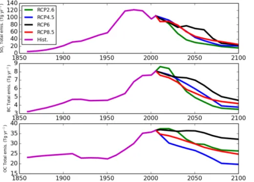
Figure 2 shows the global total emissions (anthropogenic and biomass burning) of SO₂, BC, and OC for the historical period and for each of the RCPs (see Figs. S1

15

and S2 in the Supplement for the split between anthropogenic and biomass burning). All four scenarios project strong decreases in globally averaged sulfur dioxide (SO₂), organic carbon (OC), and black carbon (BC) emissions throughout the 21st century. SO₂ emissions, according to the RCPs, have already peaked globally (around 1980) and have been on the decline since, except for a slight uptick in the early 2000 s. By

20

2100, SO₂ emissions will have decreased from a 2005 level of around 120 to 13– 26 Tg yr−1_{(RCP2.6 to RCP8.5), about an 80 % decrease. RCP2.6 projects the largest} decrease, followed by RCP4.5, RCP6, and RCP8.5. This order is consistent with each RCP’s embedded climate policy, since RCP2.6 has the most stringent climate policy and RCP8.5 the least stringent, and many climate policies that curb CO₂emissions can

25

(11)

ACPD

15, 9293–9353, 2015

Title Page

Tables Figures

◭ ◮

Back Close

Full Screen / Esc

Discussion

P

a

per

|

Discussion

P

a

per

|

Discussion

P

a

per

|

Discussion

P

a

per

|

across each of the RCPs to wield noticeable influence (Rogelj et al., 2014). Thus, cli-mate policies (specifically reductions in CO₂ emissions from reduced dependence on coal energy) tend to dominate the trend in not only emissions of aerosols and their precursors, but also in aerosol optical depth, radiative forcing, and climate response, as we will show later. Although there is some variability in global SO₂emissions over

5

the course of the time series, the RCPs all converge on a fairly narrow range of end-points. In particular, RCP6 and RCP2.6 stand out, the former due to an increase in the rate of coal consumption around mid-century (2030–2060) and the latter due to stringent climate policy including the nearly complete phase-out of non-CCS (carbon capture and storage) coal energy by roughly 2050 (Masui et al., 2011; van Vuuren

10

et al., 2011b). The increase in coal energy projected by RCP6 is a surprising feature that is not present in the other RCPs. As a result, SO₂, BC, and OC emissions in RCP6 are higher relative to the other RCPs over roughly the same time period in (Fig. 2). SO₂ emissions briefly increase in absolute terms over a short period mid-century in RCP6, which drives higher sulfate burdens, larger (negative) aerosol direct and indirect

forc-15

ings, and noticeable changes in climate response, as we will show in the following sections. The narrow range for emissions of air pollutants and their precursors (e.g. SO₂) has been attributed to similar air pollution policy assumptions in each RCP. New scenarios that strive to span the entire literature range for air pollutants in addition to greenhouse gases are undergoing development (Rogelj et al., 2014).

20

BC emissions (middle panel in Fig. 2) increased from preindustrial times and con-tinue to increase in RCP2.6, peaking around 2010. RCP4.5, RCP6 and RCP8.5 all peak around 2005 (i.e. the beginning of the RCP projections) and decrease contin-uously until 2100. Present-day values of BC emissions are 8.5 Tg yr−1_{. By 2100, BC} emissions are projected to range from less than 3.3 Tg yr−1_{according to RCP2.6 up to}

25

4.3 Tg yr−1 _{in RCP6. Here, the expected order seen in the SO}

2 emissions reductions

(12)

ACPD

15, 9293–9353, 2015

Title Page

Tables Figures

◭ ◮

Back Close

Full Screen / Esc

Discussion

P

a

per

|

Discussion

P

a

per

|

Discussion

P

a

per

|

Discussion

P

a

per

|

Emissions of OC, sometimes co-emitted with BC, have a similar trajectory (bottom panel Fig. 2). The main source of OC emissions in the RCPs is biomass burning, which makes up about 60 % of the total emissions of OC in present day. RCP2.6 OC emis-sions continue to increase in the early 21st century, peaking around 2020. Emisemis-sions of OC in RCP4.5 drop rapidly, due to the strong decrease in cropland area and increase

5

in forested area projected by RCP4.5 (in other words, a decrease in biomass burning as a means to clear cropland), a trend that is mostly unique to RCP4.5 (van Vuuren et al., 2011a; Thomson et al., 2011). OC emissions in RCP6 remain high throughout the 21st century due to the land use assumptions embedded in RCP6, which includes shifts to larger amounts of burning to clear land for crops. CO₂ fertilization also plays

10

a role in the increased emissions, as higher CO₂ levels can increase biomass growth and increase the amount available to be burned (Kato et al., 2011). Compared to SO₂ and BC, the variability and range of emissions endpoints across the different RCPs is much wider, ranging from 20 Tg yr−1 _{in RCP4.5 in 2100 to about 32 Tg yr}−1 _{in RCP6.} The final order of each RCP’s global total OC emissions is di_fferent from that of both

15

the BC and SO₂final order, highlighting the difficulty in comparison between different RCPs. In particular, the lack of climate policy in RCP8.5 has little influence on OC and BC emissions in comparison to SO₂.

2.3 Simulations

We conduct simulations using GFDL CM3 to evaluate the role of changing aerosol

20

emissions on aerosol optical depth (AOD), aerosol radiative forcing, and climate re-sponse. Table 2 summarizes the simulations performed. A series of RCP simulations (denoted RCPx.x where x.x=2.6, 4.5, etc.) were run from 2006–2100 in which the RCP emissions scenarios were used for future aerosol, greenhouse gas, and other reactive species emissions or concentrations. Another series of simulations were run

25

(13)

ACPD

15, 9293–9353, 2015

Title Page

Tables Figures

◭ ◮

Back Close

Full Screen / Esc

Discussion

P

a

per

|

Discussion

P

a

per

|

Discussion

P

a

per

|

Discussion

P

a

per

|

simulations as RCPx.x_F, where the F signifies fixed aerosol emissions. Each of the RCPx.x and RCPx.x_F simulations were run as a 3-member ensemble, each initial-ized with different initial conditions, provided by another 3-member historical ensemble (1860–2005) of GFDL CM3. The RCP4.5 and RCP4.5_F simulations are not scien-tifically di_fferent from those presented by Levy et al. (2013); however, our simulations

5

were run with a newer model version which included some minor updates. We calculate the aerosol-induced climate response as the difference between the two sets (RCPx.x – RCPx.x_F). Unless otherwise specified, all results presented are ensemble means. Meteorological factors, such as increasing temperatures, changes in atmospheric cir-culation and stability, and changes in precipitation will also induce changes in aerosol

10

concentrations (Dawson et al., 2007; Jacob and Winner, 2009; Leibensperger et al., 2012a; Pye et al., 2009; Tai et al., 2012, 2010). The influences of greenhouse-gas driven meteorological changes are included in both our RCPx.x and RCPx.x_F simu-lations. Our methodology of running the RCPx.x_F simulations for the full 21st century allows us to simulate the climate-driven e_ffects on aerosol abundance (AOD and

con-15

centration). Additionally, taking the difference between RCPx.x and RCPx.x_F isolates the changes in aerosols (and climate response) resulting from emissions reductions alone, separate from the influence of well-mixed GHG-driven climate changes. While these RCPx.x_F simulations (or analogues) were performed in some past studies, to our knowledge this is the first study to present the results from such simulations for all

20

four of the RCPs in a consistent framework.

In order to estimate aerosol effective radiative forcing, we ran additional non-coupled, atmospheric component-only simulations (AM3) in which sea surface temperatures (SST) were held constant at the 1981–2000 climatological values. Simulations were run in which the only climate forcings were aerosol emissions changes from

present-25

(14)

ACPD

15, 9293–9353, 2015

Title Page

Tables Figures

◭ ◮

Back Close

Full Screen / Esc

Discussion

P

a

per

|

Discussion

P

a

per

|

Discussion

P

a

per

|

Discussion

P

a

per

|

a forcing agent (e.g., aerosols) in addition to the full? response to the forcing agent itself. This method accounts for the indirect e_ffects of aerosols, including the cloud life-time effect and the cloud albedo effect. This type of fixed-SST calculation has been referred to as the “radiative flux perturbation” (Lohmann et al., 2010) or “effective radia-tive forcing” (Myhre et al., 2013). This series of simulations are denoted RCPx.x_RFP

5

for the aerosol-only simulations and RCP_1860 for the control simulation. This pair of simulations is only used for the radiative forcing calculations, while the coupled runs described above provide AOD and climate response estimates.

3 Global analysis

We first focus our analysis on area-weighted global means ranging from pre-industrial

10

times to 2100. We analyze aerosol optical depth (sulfate, BC, and OC), aerosol climate forcing (direct and indirect), and climate response (temperature, precipitation rate, liq-uid water path, and effective cloud droplet radius). In subsequent sections, the analysis is extended to examine spatial distributions and mean changes over specific regions. Past, present, and future trends in global aerosol optical depth can be found in the

15

Supplement, Sect. S2 as well as Figs. S3 and S4. In short, AOD trends are well cor-related with emissions trends, with correlation coe_fficients ranging from 0.7 to 0.9 for each species and each RCP (not shown). By 2100, sulfate AOD globally is projected to decrease by 50 % from 2005 levels in RCP2.6, 40 % in RCP4.5 and RCP6, and 31 % in RCP8.5 (see the Supplement). Figure S3 shows the RCPx.x_F fixed emissions

sim-20

ulations (dashed lines) along with the RCPx.x decreasing emissions runs (solid lines) indicating that in the absence of emissions changes, future climate changes cause AOD to increase globally for each of the RCPs. However, this climate driven e_ffect is small compared to the substantial decrease in AOD from emissions reductions (com-pare dashed and solid lines in Fig. S3).

(15)

ACPD

15, 9293–9353, 2015

Title Page

Tables Figures

◭ ◮

Back Close

Full Screen / Esc

Discussion

P

a

per

|

Discussion

P

a

per

|

Discussion

P

a

per

|

Discussion

P

a

per

|

3.1 Aerosol forcing

3.1.1 Aerosol direct and indirect forcing

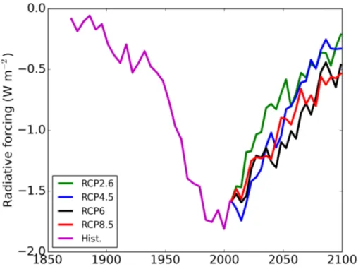
Changes (mostly decreases) in aerosol emissions and aerosol amount and optical depth lead to changes in Earth’s radiative balance. Figure 3 shows the globally av-eraged total top-of-atmosphere (TOA) aerosol forcing (direct and indirect) for the

his-5

torical period and four RCP projections. From 1860 until present day, the increasing abundance of atmospheric aerosols led to a larger (more negative) aerosol forcing, peaking near present day. Preindustrial to present day aerosol forcing simulated by CM3 is about−1.8 W m−2. This large negative forcing has offset or “masked” some of

the positive forcing from greenhouse gases. Although the net forcing is still positive,

10

without the large increase in the 20th century of aerosol emissions, the net positive forcing would be much larger. As we discuss in Sect. 3.2, this masking by aerosols of the positive, greenhouse gas warming has important implications for climate. During the 21st century, the large decreases in global aerosol and aerosol precursor emis-sions projected by the RCPs cause aerosol forcing to decrease in magnitude (become

15

less negative).

As in many of the other trends shown thus far, there is limited spread in the various RCP projections of global aerosol effective radiative forcing (Fig. 3). For the 2096–2100 five-year average, the e_ffective forcing (relative to 1860) is ₋0.21 for RCP2.6, ₋0.32 for RCP4.5,−0.46 for RCP6, and −0.53 W m−2 for RCP8.5. RCP2.6 has the largest 20

decrease in magnitude of aerosol forcing over the century, followed by RCP4.5, RCP6, and RCP8.5, which is the expected order according to each RCP’s underlying climate policy. For example, reduction of coal energy usage, a GHG mitigation policy featured in the RCPs, also reduces the amount of SO₂ emissions. As a result, total aerosol forcing trends and the end-of-century rank order for each of the RCPs can be traced

25

(16)

ACPD

15, 9293–9353, 2015

Title Page

Tables Figures

◭ ◮

Back Close

Full Screen / Esc

Discussion

P

a

per

|

Discussion

P

a

per

|

Discussion

P

a

per

|

Discussion

P

a

per

|

policies that affect sulfate will have a magnified effect on aerosol direct and indirect forcing. On the other hand, the direct climate e_ffects of BC and OC have been reported to offset each other (OC being the negative forcing, BC positive) in previous studies with CM3 (Levy et al., 2013), and that is the case in this work as well. RCP6 projects the smallest decrease in magnitude of aerosol forcing for much of the middle part of the

5

century (2045–2075), despite passing RCP8.5 eventually. This is consistent with both the emissions and AOD trajectories for RCP6. RCP6 projects mid-century increases in coal for energy supply globally (Masui et al., 2011), which is visible not only in the emissions and AOD trends as described elsewhere but also the aerosol forcing trends.

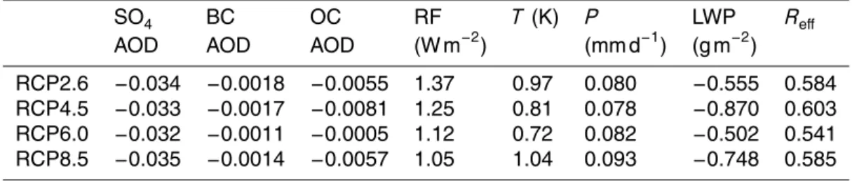
3.1.2 Comparison to 2005 levels

10

The large decrease in the magnitude of aerosol forcing from present-day to 2100 repre-sents a largepositiveforcing for 2100 relative to present. The globally averaged forcing changes from present-day to year 2100 for each RCP scenario are tabulated in Table 3. In order to have a consistent basis for comparison across the four RCPs and to account for noise in the trends, the beginning and end of century forcing values were taken as

15

5-year averages, 2000–2004 and 2096–2100. The amount of unmasked aerosol forc-ing follows the order expected accordforc-ing to each RCP’s climate policy (as explained above), as is the case with SO₂emissions (Fig. 2). For RCP2.6, the forcing increases by 1.37 W m−2 _{from 2000 to 2100. RCP8.5 represents the lower part of the range at} 1.05 W m−2_{. An additional positive forcing of at least 1 W m}−2_{would have major climate}

20

implications. For comparison, the present day CO₂forcing is about 1.68 W m−2_(range of 1.33 to 2.03 W m−2_{) (Myhre et al., 2013). Thus, the resulting positive forcing from the} decrease in aerosol emissions by 2100 is projected to be more than half of the forcing of present day CO₂.

As a caveat, our reported forcing values may be a slight overestimate due to the

25

(17)

ACPD

15, 9293–9353, 2015

Title Page

Tables Figures

◭ ◮

Back Close

Full Screen / Esc

Discussion

P

a

per

|

Discussion

P

a

per

|

Discussion

P

a

per

|

Discussion

P

a

per

|

In a multimodel evaluation of proxies for the aerosol indirect effects (both albedo and lifetime) against satellite observations, a prototype version of AM3 was found to be one of several models overestimating the strength of the relationship between cloud liquid water path (LWP) and aerosol optical depth (defined as sensitivity of LWP to AOD per-turbations) (Quaas et al., 2009). Ratios for AM3 were roughly an order of magnitude

5

larger than observations over land and ocean; however, other models performed just as poorly if not worse (all models overestimate the land ratio by at least a factor of two). Generally, a positive correlation is expected between aerosol optical depth and cloud liquid water path, since the increase in cloud droplet number concentration leads to a delay in autoconversion rate, increasing cloud lifetime and cloud liquid water path.

10

However, some studies have found potential for a negative correlation due to a dry-ing effect from increased entrainment of air above the clouds (Ackerman et al., 2004). Thus, the autoconversion parameterization in AM3, which is a simple implementation that does not address the e_ffect of increased entrainment and other confounding is-sues, could conceivably be driving an overestimate in the cloud lifetime e_ffect and thus

15

the indirect effect as a whole.

3.2 Climate response

3.2.1 Global historical and future trends

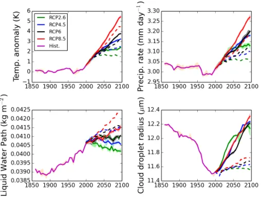
The emission reductions and aerosol forcing trends discussed earlier will have signif-icant e_ffects on future climate. Figure 4 shows the 1860–2100 globally averaged time

20

series for temperature, precipitation rate, liquid water path, and effective cloud droplet radius for the historical, RCPx.x ensemble mean (solid lines), and RCPx.x_F ensemble mean (dashed lines). Since the RCPx.x simulations contain all climate-forcing agents (compared to the aerosol di_fferences we will discuss later), greenhouse gases have a large influence. Temperature anomaly (relative to 1881–1920 average) is projected

25

(18)

follow-ACPD

15, 9293–9353, 2015

Title Page

Tables Figures

◭ ◮

Back Close

Full Screen / Esc

Discussion

P

a

per

|

Discussion

P

a

per

|

Discussion

P

a

per

|

Discussion

P

a

per

|

ing section to result partially from an increase in greenhouse gases and a decrease in aerosol emissions. Precipitation rate in the historical simulation had a significant decrease around 1950–1970; this time frame coincides with a doubling in the global anthropogenic SO₂ emissions (Fig. 2). Liquid water path (LWP) (Fig. 4, bottom left) steadily increases from 1860 to present day, then has four very di_fferent trajectories in

5

the RCP future projections. The higher temperatures of RCP8.5 and RCP6 most likely lead to LWP increases, and the order of LWP values in each RCP in 2100 is consis-tent with the amount of temperature increase. E_ffective cloud droplet radius (calculated over the top two units of optical depth for liquid clouds, consistent with the Moderate Resolution Imaging Spectroradiometer (MODIS) algorithm (Donner et al., 2011; Guo

10

et al., 2014; King et al., 2003) and weighted by cloud fraction) decreases steadily from 1950 to present day, also due to the large increase in aerosol emissions. Since many ultrafine particles are anthropogenic in nature (e.g., sulfate), an increase in their emis-sion drives down the global average cloud droplet e_ffective radius, since smaller sized aerosols are e_ffective CCN that are likely to activate into cloud droplets. Likewise, with

15

aerosol emissions declining in the 21st century, cloud droplet radius increases across all of the RCPs.

3.2.2 Climate response to aerosol forcing

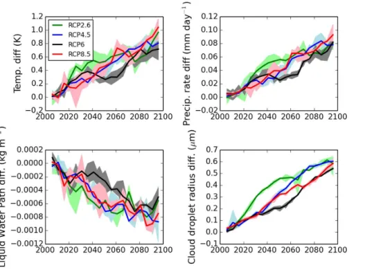
As with aerosol optical depth, taking the difference between the time-varying simu-lations discussed in Sect 3.3.1 and the fixed aerosol emission simusimu-lations (RCPx.x

20

– RCPx.x_F), we deduce the impacts on climate driven solely by the aerosol emis-sions reductions for each year of each future emission scenario. Figure 5 presents the globally-averaged differences for temperature, precipitation rate, cloud cover, and cloud drop e_ffective radius resulting from aerosol emission reductions in the RCPs (also tab-ulated in Table 3 for a five year average of 2096–2100 only). Additionally, the dashed

25

(19)

ACPD

15, 9293–9353, 2015

Title Page

Tables Figures

◭ ◮

Back Close

Full Screen / Esc

Discussion

P

a

per

|

Discussion

P

a

per

|

Discussion

P

a

per

|

Discussion

P

a

per

|

projected global temperature increase due to aerosol emissions reduction alone ranges from 0.72 to 1.04 K, compared to 2005 temperature levels. This is a significant fraction of thetotaltemperature increase by 2100 (including greenhouse gas induced warming) of 1–5 K across the RCPs (compare dashed and solid lines in Fig. 4). This is discussed in more detail in Sect. 4.1.3 and shown in Fig. 8. The impact of the RCP2.6

aggres-5

sive phase-out of coal as an energy source can be seen from about 2020–2050 with a strong increase in aerosol driven temperature change. Likewise, the mid-century rise in coal use in RCP6 shows up as a decline in what is an otherwise consistent tem-perature increase throughout the century (Fig. 5). RCP4.5 and RCP8.5, on the other hand, have a steadier temperature increase that lacks the same noticeable features.

10

There is a significant amount of overlap in climate response from decreasing aerosols among the RCPs throughout the entire century, especially considering the full range of the ensemble members of each simulation. This suggests that despite large di_ff er-ences in many facets of the individual RCPs (e.g., climate mitigation policies, emissions trajectories, land use), the temperature response to decreasing aerosols is relatively

15

homogenous.

Although global precipitation rate (Fig. 5 upper right) is mainly controlled by the tro-pospheric energy balance (Ming et al., 2010), precipitation is linked to aerosols on the local scale, since aerosols serve as seeds for cloud droplet formation and the number and size of the cloud droplets influence the precipitation rate. Additionally, aerosols can

20

impact precipitation in other ways, including by changing atmospheric dynamics and circulation patterns, changing atmospheric heating rates, and changing the surface en-ergy balance. We find increases of 0.08–0.09 mm d−1 _{(up to 3 % of 2005 precipitation} levels) are projected to result from the aerosol decrease in the four RCPs, again rep-resenting a very narrow range of climate endpoints despite the di_fferences among the

25

(20)

consis-ACPD

15, 9293–9353, 2015

Title Page

Tables Figures

◭ ◮

Back Close

Full Screen / Esc

Discussion

P

a

per

|

Discussion

P

a

per

|

Discussion

P

a

per

|

Discussion

P

a

per

|

tent with the finding by Shindell et al. (2012) that precipitation responds more strongly to aerosol forcing than an equivalent CO₂forcing.

Liquid water path differences over time are shown for each of the RCPs in the lower left panel of Fig. 5. As aerosol concentrations decrease, LWP also decreases; in other words, aerosols and LWP are positively correlated. This is essentially the cloud lifetime

5

effect acting in the opposite direction: increased aerosols cause cloud droplet concen-trations to increase leading to a decrease in the autoconversion rate, which hinders precipitation formation and increases cloud lifetime and cloud liquid water path (Al-brecht, 1989). The decline in aerosol emissions leads to a decrease in LWP in all of the RCPs, around 0.5–1.0 g m−2 _{or 2 % of 2005 levels. Accounting for the ensemble}

10

member range (shaded areas), the LWP decline in each of the RCPs is remarkably similar. As is the case with radiative forcing, temperature, and precipitation, the annual trends in the LWP values also follow the underlying RCP energy use trajectories. In particular, a rebound around 2040 in LWP in RCP6 can be seen in the bottom left of Fig. 5, analogous to the temperature decrease in RCP6 due to an increase in coal

15

energy usage rate and ultimately aerosol and precursor emissions.

With decreasing aerosols, e_ffective cloud drop radius may increase due to the loss of smaller-sized and more numerous anthropogenic ultrafine aerosol, leaving natural aerosols (such as sea spray, which in general are fewer in number and much coarser in size) to form cloud droplets. Across the four RCPs, the globally averaged increase

20

in cloud drop e_ffective radius due to decreasing aerosols ranges from 0.54 to 0.60 µm (Fig. 5, Table 3). The increase due to all forcings ranges from about 0.60–0.80 µm (Fig. 4). As expected, the increases in cloud droplet e_ffective radius due to aerosol reductions make up a large fraction of the all-forcing increases. Cloud droplet e_ffective radius trends follow energy usage and emissions trends in each of the RCPs very

25

(21)

ACPD

15, 9293–9353, 2015

Title Page

Tables Figures

◭ ◮

Back Close

Full Screen / Esc

Discussion

P

a

per

|

Discussion

P

a

per

|

Discussion

P

a

per

|

Discussion

P

a

per

|

4 Spatial distribution and regional analysis

Emissions of aerosols and aerosol precursors are highly heterogeneous in space. As expected, the changes of AOD, radiative forcing, and climate change in response to projected future emission changes also exhibit strong spatial structure. In this section, we first examine the spatial distributions of the changes in AOD and climate response,

5

and then consider the average responses over two key source regions, East Asia and North America. Judging by historical emissions over the last few years since the RCPs were developed, concentrations of GHG in the atmosphere are tracking at or even above the trajectory predicted by RCP8.5 (the highest emission scenario), so we will focus mainly on that scenario (Peters et al., 2012; Sanford et al., 2014).

10

4.1 Spatial distributions

4.1.1 Aerosol optical depth

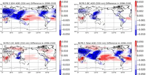
Figure 6 shows the RCP8.5 aerosol optical depth (550 nm) di_fferences (RCP8.5 – RCP8.5_F) for the end of the 21st century (2096–2100 average) for sulfate, BC, OC, and total AOD. Corresponding results for the other three RCPs can be found in

15

Figs. S6–S8. Strong reductions in AOD are simulated over most continental regions, including North America, Europe, and Asia. This coincides with the strong SO₂ emis-sions decreases projected by RCP8.5 (and all RCPs) for much of the world. East and South Asia have the largest and most widespread decreases in AOD for all species. However, there are a few regions in which emissions changes are projected toincrease

20

sulfate AOD by 2100. Africa has noticeable areas of sulfate AOD increase, which can be explained by RCP8.5 projected increases in emissions at a few locales in this re-gion (see Fig. S5). Parts of Africa are expected to industrialize and grow throughout the rest of the century and utilize its natural fossil fuel resources (Masui et al., 2011; Riahi et al., 2007). Similarly, RCP8.5 projects sulfate AOD increases for Indonesia, a region

25

(22)

ACPD

15, 9293–9353, 2015

Title Page

Tables Figures

◭ ◮

Back Close

Full Screen / Esc

Discussion

P

a

per

|

Discussion

P

a

per

|

Discussion

P

a

per

|

Discussion

P

a

per

|

resulting in elevated emissions of SO₂, BC, and OC. There are also a few areas of increase over the tropical Pacific and Atlantic oceans for OC and SO₂ which are not caused by emissions increases (see Fig. S5) and instead result from meteorological changes, specifically a decrease in effectiveness of wet deposition removal of sulfate and OC. Since precipitation is increasing along with sulfate and OC aerosol optical

5

depth, a decrease in the efficacy of wet deposition is implied. Although we do not have wet deposition fluxes archived in the model output, we note that using the same model, Fang et al. (2011) confirmed this relationship between increasing precipitation and de-creasing wet deposition removal effectiveness. Using an idealized soluble tracer, the authors found that as climate warms, wet deposition of soluble pollutants decreases

10

due to the simulated decreases in large-scale precipitation over land, suggesting that global large-scale precipitation changes are not a good indicator of the changes in wet scavenging of soluble species (Fang et al., 2011).

Asian BC and OC AOD decreases by 2100 are much larger than those in North America or Europe (Fig. 6). Some increases are again projected in Africa. BC and OC

15

biomass burning emissions on average in Africa are generally expected to maintain current levels or decline slightly; however, in this particular region of Africa (mostly in Democratic Republic of the Congo and the Central African Republic), biomass burning emissions of OC and BC are projected to rise (not shown, see Fig. S5). In particular, combustion and biomass burning emissions in Africa are expected to increase rapidly

20

in the near-term (Liousse et al., 2014). The total AOD di_fference in 2100 for RCP8.5 (lower right of Fig. 6) is dominated by the sulfate AOD reductions over the continents (except for in parts of Africa and other developing regions).

4.1.2 Climate response

The climate responses to the aerosol reductions in RCP8.5 are shown in Fig. 7 for the

25

(23)

ACPD

15, 9293–9353, 2015

Title Page

Tables Figures

◭ ◮

Back Close

Full Screen / Esc

Discussion

P

a

per

|

Discussion

P

a

per

|

Discussion

P

a

per

|

Discussion

P

a

per

|

in each of the figures indicate statistically significant regions at the 95 % confidence level according to Student’st test. For temperature (upper left), the impact of aerosol reductions is almost entirely a warming effect, as expected, and nearly all of these in-creases are statistically significant. There are large areas of temperature increase in 2100 for East Asia, which is consistent with the largest decreases in AOD and aerosol

5

emissions in this region. However, much of the strongest temperature increases driven by reduced aerosol emissions are located in or near the Arctic, suggesting that temper-ature change is non-local and does not necessarily occur in the areas where emissions are changing. Shindell et al. (2010) also have reported strong temperature increases in the Arctic where forcing was small in a global multimodel study.

10

Precipitation rate increases due to decreased aerosol emissions are largest over the tropical oceans, although increases are also observed over continents. In particular, some statistically significant precipitation rate increases occur over Europe, Russia, and Southeast Asia. Increases over North America are generally not found to be tistically significant. However, much of the areas of increase over the oceans are

sta-15

tistically significant. Simulating precipitation, especially regional details, remains chal-lenging for most models, including CM3 (Eden et al., 2012). In our results there are two intercontinental tropical convergence zones (ITCZ) near the equator, a common fea-ture not only identified in CM3 but in other models as well (Lin, 2007). Both of the ITCZ show strong areas of precipitation enhancement despite not coinciding with aerosol

de-20

creases. Precipitation in the tropics is mainly a result of deep convection, and several studies have identified the effect of aerosols on deep convective circulation and pre-cipitation (Bell et al., 2008; Lee, 2012; Rosenfeld et al., 2008). Using a cloud-system resolving model of a large-scale deep convective system, Lee (2011) found that pertur-bations of aerosols in one domain can have teleconnections to other domains, acting

25

(24)

ACPD

15, 9293–9353, 2015

Title Page

Tables Figures

◭ ◮

Back Close

Full Screen / Esc

Discussion

P

a

per

|

Discussion

P

a

per

|

Discussion

P

a

per

|

Discussion

P

a

per

|

aerosol indirect effect alone. The aerosols are also likely exerting an influence on at-mospheric dynamics and weather patterns, causing large, non-uniform increases and decreases in the tropics. In particular, we postulate that the aerosol decreases in the continental domain are having teleconnections to deep convection, resulting in both precipitation increases and decreases, as demonstrated by Lee (2011).

5

Liquid water path changes (Fig. 7, lower left panel) are largest over East Asia, which again is consistent with the simulated aerosol changes. Much of Europe and eastern North America also have large LWP decreases that coincide with aerosol emission de-creases. However, there are large LWP increases in the Arctic region, most of which are statistically significant. These increases are most likely due to a feedback from

10

the aerosol-driven temperature increase, since warmer air can hold more moisture. Cloud droplet radius increases universally across the globe, with statistically signifi-cant changes occurring in the Northern Hemisphere, which is also where most of the aerosol reductions occur (Fig. 7, lower right). The co-location of the large increases in cloud droplet e_ffective radius with large decreases in aerosol optical depth is a strong

15

signal of the aerosol indirect effect, specifically the cloud albedo effect (we will explicitly show this with correlations in Sect. 5). Since the impacts of aerosol reductions on both liquid water path and cloud droplet e_ffective radius are significant over the oceans in addition to the continents, we can also conclude that the aerosol reduction impacts are not necessary localized to their area of emission. Additionally, the increases of cloud

20

droplet radius over the oceans may be amplified due to the greater susceptibility of clouds in clean environments compared to more polluted conditions.

4.1.3 Comparison of climate response driven by aerosol decreases and by all

forcings

Although the projected absolute climate response to decreasing aerosols is similar in

25

(25)

ACPD

15, 9293–9353, 2015

Title Page

Tables Figures

◭ ◮

Back Close

Full Screen / Esc

Discussion

P

a

per

|

Discussion

P

a

per

|

Discussion

P

a

per

|

Discussion

P

a

per

|

decreases to the total changes in climate for each RCP. The nonlinear nature of the global climate system means that these aerosol ratios are not directly additive with other ratios (say, GHG-induced climate changes) and are not the “true contributions” per se. However, comparing the magnitudes of the aerosol-induced climate changes to the total climate changes is a useful framing exercise. For example, we project from

5

2006 to the end-of-century a 0.97 K warming from aerosol emissions reductions in RCP2.6 (Fig. 5, Table 3) compared with a 1.5 K warming from all climate forcings to-gether (Fig. 4), indicating that, under this scenario, two-thirds of the warming by 2100 would result from decreases in aerosol emissions. The RCP2.6 scenario indicates that even with aggressive reductions in the emissions of greenhouse gases, the projected

10

reduction in aerosol emissions is likely to push the climate near the 2 K warming fre-quently cited as constituting “dangerous anthropogenic interference with the climate system” (Meinshausen et al., 2009). Since RCP2.6 projects the least warming from greenhouse gases, we find that this scenario is relatively the most susceptible (i.e. the largest percent e_ffect) to unmasked aerosol warming as well as aerosol-driven changes

15

in precipitation, LWP, and cloud droplet effective radius.

However, since emissions over the past decade have been well above RCP2.6 and even slightly above RCP8.5 (Peters et al., 2012; Sanford et al., 2014), using RCP2.6 as a benchmark for the aerosol fraction of future climate change may be misleading. Figures 4 and 5 show that for RCP8.5, warming from aerosol reductions is roughly 1 K

20

globally of a total warming of nearly 5 K, or around 20 %. The RCP8.5 precipitation in-crease of 0.09 mm d−1_{is about 36 % of the all-forcing increase of}

∼0.25 mm d−1, while

the globally averaged ratios for LWP and cloud droplet e_ffective radius are 30 and 75 %, respectively. The large aerosol fraction for cloud droplet radius is expected, since cloud droplet size is highly dependent on existing aerosols, perhaps to a greater extent than

25

(26)

ACPD

15, 9293–9353, 2015

Title Page

Tables Figures

◭ ◮

Back Close

Full Screen / Esc

Discussion

P

a

per

|

Discussion

P

a

per

|

Discussion

P

a

per

|

Discussion

P

a

per

|

Figure 8 shows the spatial distribution for 2096–2100 five-year averages of the ra-tio of aerosol-driven climate response to total climate response. Surface temperature increases due to aerosols are a substantial fraction of the all-forcing warming, even in RCP8.5 which features the largest warming from long-lived greenhouse gases. Much of East Asia, Australia, and the Middle East have ratios above 30 %, indicating that the

5

large aerosol decreases in these regions will contribute significantly to projected warm-ing. Even over the oceans, where anthropogenic aerosol abundances are low, their global decrease accounts for more than 10–20 % of the all-forcing warming in these locations. Precipitation ratios are not as smoothly distributed as temperature. Ratios are near 100 % over the extra-tropical Pacific Ocean and Indian Ocean, whereas ratios

10

over most of the Southern and Arctic Oceans are near 0. Parts of East Asia and Eu-rope, regions for which major aerosol decreases are expected, have ratios approaching 100 %; however, this is not generalizable to all continental regions. Like precipitation, LWP ratios are close to 0 near the poles, with sporadic regions of large LWP ratios, indicating larger aerosol influence compared with all-forcings in these regions. Finally,

15

ratios for cloud droplet radius approach 100 % for much of the globe between the lati-tudes 30◦_{S and 60}◦_{N. Ratios are particularly low in the Southern Ocean, where natural} aerosols such as sea salt likely dominate CCN activation, and thus are less a_ffected by decreasing anthropogenic aerosols.

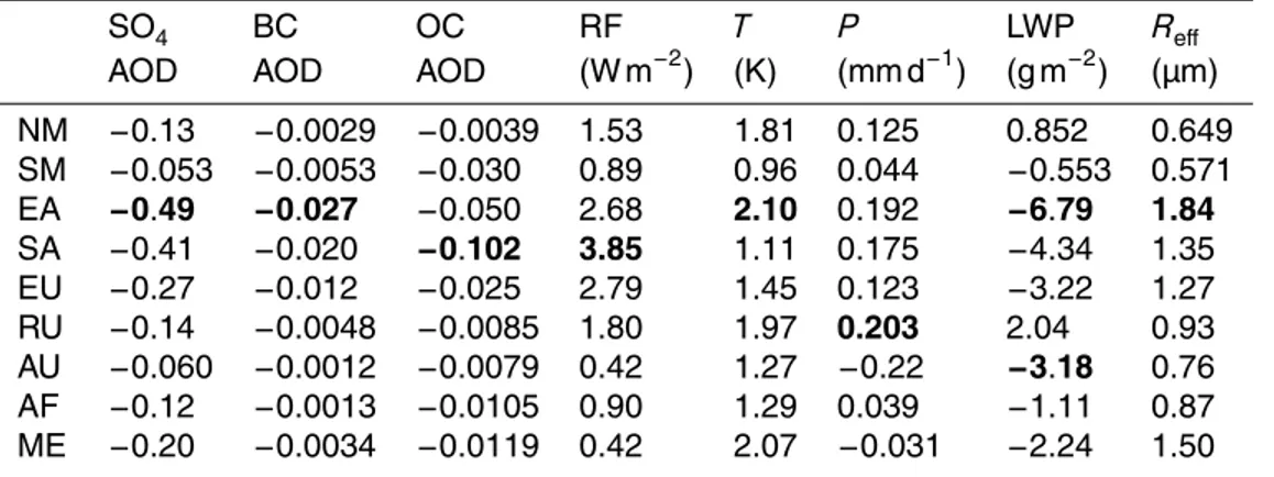
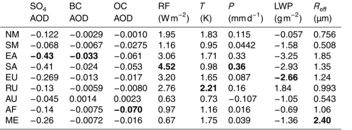
4.2 Regional climate response

20

Using the regions defined in Fig. 1, we quantify changes in AOD, radiative forcing, and climate responses due to changes in aerosol concentrations on a regional scale in Tables 4 and 5. We present the effective radiative forcing (or flux perturbation) as a dif-ference between the 2096–2100 value and the 2000–2004 levels (as before), which is why these values are mostly positive. The AOD and climate di_fferences are the di_ff

er-25

(27)

ACPD

15, 9293–9353, 2015

Title Page

Tables Figures

◭ ◮

Back Close

Full Screen / Esc

Discussion

P

a

per

|

Discussion

P

a

per

|

Discussion

P

a

per

|

Discussion

P

a

per

|

upper and lower ranges of AOD, radiative forcing, and climate response changes. Iden-tical tables for RCP4.5 and RCP6 can be found in the Supplement (Tables S1 and S2). Bolded values in the tables represent the largest regional change for each quantity (e.g., largest SO₄AOD decrease).

4.2.1 East Asia

5

Several of the largest aerosol-driven climate changes are found in the East Asian re-gion. The region is defined to include all of China, Mongolia, Japan, and Korea (Fig. 1). East Asian emissions, AOD, radiative forcing, and climate response are analyzed be-low.

Figure S12 shows the anthropogenic SO₂, BC, and OC emissions time series from

10

East Asia for the historical period and for each of the RCPs. For all species and all RCPs except RCP6, aerosol and aerosol precursor emissions are projected to peak in the 2010 s. The trend for RCP6 for each species consists of a small increase in the 2010 s, followed by a brief decrease and then a sharp increase with emissions peaking in 2050. This shifted trend results from the primary energy supply projections in RCP6,

15

in which coal energy usage in East Asia increases steadily until peaking in 2050–2060. This reliance on coal as a primary fuel source results in a mid-century peak in not only aerosol and precursor emissions, but also CO₂emissions (Masui et al., 2011).

Figure S13 shows the East Asian region aerosol radiative forcing (calculated as a flux perturbation or effective radiative forcing) for all the RCPs and the historical period. This

20

calculation is done by simply averaging over the region considering global aerosols as opposed to isolating the e_ffect of East Asian aerosols alone. Radiative forcing from aerosols (direct + indirect) will continue to become more negative (larger in magni-tude) until about 2025, when it reaches nearly₋5 W m−2_{over the region. For the rest} of the century, the decrease in aerosol emissions (and AOD) results in a less negative

25