© Author(s) 2007. This work is licensed under a Creative Commons License.
Chemistry
and Physics
Global trends in visibility: implications for dust sources
N. M. Mahowald1, J. A. Ballantine2,*, J. Feddema3, and N. Ramankutty4
1National Center for Atmospheric Research, Boulder Colorado, USA
2Institute for Computational Earth System Science, University of California, Santa Barbara, CA, USA 3Department of Geography, University Kansas, Lawrence, Kansas, USA
4Department of Geography, McGill University, Montreal, Quebec, Canada *now at: United States Geological Survey, Denver, Colorado, USA
Received: 8 January 2007 – Published in Atmos. Chem. Phys. Discuss.: 27 February 2007 Revised: 23 May 2007 – Accepted: 15 June 2007 – Published: 26 June 2007
Abstract. There is a large uncertainty in the relative roles of human land use, climate change and carbon dioxide fer-tilization in changing desert dust source strength over the past 100 years, and the overall sign of human impacts on dust is not known. We used visibility data from meteoro-logical stations in dusty regions to assess the anthropogenic impact on long term trends in desert dust emissions. We did this by looking at time series of visibility derived variables and their correlations with precipitation, drought, winds, land use and grazing. Visibility data are available at thousands of stations globally from 1900 to the present, but we focused on 357 stations with more than 30 years of data in regions where mineral aerosols play a dominant role in visibility ob-servations. We evaluated the 1974 to 2003 time period be-cause most of these stations have reliable records only dur-ing this time. We first evaluated the visibility data against AERONET aerosol optical depth data, and found that only in dusty regions are the two moderately correlated. Corre-lation coefficients between visibility-derived variables and AERONET optical depths indicate a moderate correlation (0.47), consistent with capturing about 20% of the variability in optical depths. Two visibility-derived variables appear to compare the best with AERONET observations: the fraction of observations with visibility less than 5 km (VIS5) and the surface extinction (EXT). Regional trends show that in many dusty places, VIS5 and EXT are statistically significantly correlated with the Palmer drought severity index (based on precipitation and temperature) or surface wind speeds, con-sistent with dust temporal variability being largely driven by meteorology. This is especially true for North African and Chinese dust sources, but less true in the Middle East, Aus-tralia or South America, where there are not consistent pat-terns in the correlations. Climate indices such as El Nino or the North Atlantic Oscillation are not correlated with
Correspondence to:N. M. Mahowald ([email protected])
visibility-derived variables in this analysis. There are few stations where visibility measures are correlated with culti-vation or grazing estimates on a temporal basis, although this may be a function of the very coarse temporal resolution of the land use datasets. On the other hand, spatial analysis of the visibility data suggests that natural topographic lows are not correlated with VIS5 or EXT, but land use is correlated at a moderate level. This analysis is consistent with land use being important in some regions, but meteorology driving in-terannual variability during 1974–2003.
1 Introduction
of global scale anthropogenic land use on dust emissions are hampered by the similarity in the spatial distribution of land use derived dust and natural dust for some sources (e.g. Ma-howald et al., 2002, 2004; Luo et al., 2003). Results of mod-eling simulations suggest that humans have either increased or decreased dust since preindustrial times, depending on the relative importance of human land use, carbon dioxide fer-tilization and climate change in driving dust (Mahowald and Luo, 2003). Ice core changes between the preindustrial and current time periods are not consistent within regions and cannot differentiate between these different processes (Ma-howald and Luo, 2003).
One long time series that is globally available is visibility data collected at meteorological stations. It has been used in many previous studies (e.g. Middleton, 1984; McTainsh et al., 1989; Goudie and Middleton, 1992; Sun et al., 2001). However, visibility data have not been compiled and pre-sented globally with time trends in previous studies. These data are available at hourly to several times daily intervals over much of the last century at many meteorological sta-tions located throughout the world. One problem with these data is that visibility is not directly related to aerosol con-centration, but may be influenced by humidity, cloudiness or rain. Visibility is a function of the amount of light which is attenuated as a viewer looks horizontally, and if the attentua-tion is due to aerosols, it is the extincattentua-tion of light by aerosols occuring at the surface of the earth (surface extinction). In addition, aerosol amount near a station may be impacted by very local effects, such as the existence of a dirt road directly in front of the observer (e.g. Middleton et al., 1985). Another drawback of the visibility data is that while there are hun-dreds of stations, they are located close to human habitation, which tends not to be in the middle of deserts. Traditionally researchers have considered visibility as too qualititavely to be compared against models or other data. In this paper we try to address how quantitatively we can use the visibility data, and especially whether it represents very local dust or dust capable of being transported long range. Thus as a first step in our analysis, we compared the visibility data against other high quality aerosol data (AERONET aerosol optical depths: Holben et al., 2001) to understand the quantitative value of this dataset. Our goal in the first part of the paper is to determine whether visibility data can be used to evalu-ate dustiness, and what relationship the visibility data has to surface source variability.
Many processes may be important for the generation of atmospheric dust, including strong winds, precipitation, drought conditions, land surface properties, and human land use. For each of these processes we try to derive a repre-sentative proxy from a global dataset to correlate with the visibility dataset. However, this approach has fundamen-tal limitations due to lack of quality data. There is a large spatial variability in surface winds and precipitation, mak-ing these variables difficult to constrain globally (e.g. Dai et al., 1996). Very little is known globally about land surface
properties, and we address these in a future study. Especially problematic are datasets on the time evolution of human cul-tivation and grazing. The datasets used here present a broad view of the time evolution of cultivation and grazing, and represent the best datasets available (Klein-Goldewijk, 2001; Ramankutty and Foley, 1999). However they are interpola-tions between land use censuses taken every 5 years in the best case, and often every 10 years or longer, and therefore crudely represent the time record of human land use. In ad-dition, it is not clear how human land use would impact dust. Some studies have shown that cultivation and grazing make soils much easier to deflate (Gillette, 1988; Neff et al., 2005). Soil conservation efforts such as trees planted to block the winds, contour plowing, and leaving dead vegetation on the top of the soils have been shown to be effective in reducing wind erosion (e.g. Baker et al., 2005). Thus, it is not always straightforward to deduce what the relationship should be be-tween human land use and dust. This paper may provide some information about where land use may be enhancing dust sources.
Our goal in this paper is to use visibility data for esti-mating long term trends in aerosols, especially desert dust aerosols. We describe our methods in Sect. 2. We first evaluate several proxies derived from the hourly visibility data against AERONET column aerosol optical depth data in Sect. 3. Then we use visibility proxies to look at tempo-ral trends in dusty regions. Finally, we correlate visibility proxies with meteorological variables such as precipitation and wind speeds as well as the human driven variables, es-timated cultivation and grazing use (Sect. 4). Summary and conclusions are presented in Sect. 5.
2 Methodology
For this paper, we analyze hourly to several times daily station data from the DSS 463.3 surface weather observa-tion dataset created by the Naobserva-tional Climatic Data Center (NCDC) and archived at NCAR (http://dss.ucar.edu/datasets/ ds463.3/). This data set contains up to 10 000 active stations worldwide. We analyze this dataset over the period 1900– 2003 for long term trends in visibility. For the bulk of the analyses, we include stations with data in at least 30 years of the period from 1900–2003. In dusty regions, where most of our analysis takes place, there are no data before 1940, so we do not focus on that time period. Indeed, there are substan-tially more data from 1974–2003, so we concentrate much of our correlation analysis on that time period, discussing only briefly results for the longer time period.
are neglected here. We also visually inspect the different sta-tion time series to look for discontinuities in the data, specif-ically in the wind data, and rejected 7 stations due to this problem (WMO stations 400720, 400830, 400870, 607600 612970 847820 and 854170). In addition, we exclude any data when the dew point temperature is within one degree Celsius of the temperature to attempt to exclude fog events. There are over one thousand stations with data for at least 30 years, but only 364 stations with more than 30 years of data in dusty regions (we discuss the reasons for focussing on dusty regions in Sect. 2.0).
In order to evaluate the visibility measurements, we com-pare them against data from AERONET sun photometry stations, which are in situ column optical depth measure-ments (Holben et al., 2001) (http://aeronet.gsfc.nasa.gov/ data menu.html). Because we are interested in variability in visibility, we only use the data from AERONET stations with more than 3 years of data, and we calculate the correla-tion coefficient between monthly mean aerosol optical depth at 670 nm and monthly visibility proxies at the closest me-teorological stations. We chose this wavelength because it appears to have the most data, and varies in a manner similar to other visible wavelengths in the same dataset (not shown). We evaluate several different visibility proxies at the AERONET sites. The fraction of observations when the visibility is less than 1, 5, or 10 km has been used previ-ously (e.g. N’Tchayi Mbourou et al., 1997; Kurosaki and Mikami, 2003). We evaluate the fraction of visibility be-low a succession of thresholds between 1 and 10 km to de-termine which best reproduces the column aerosol optical depth from AERONET. In addition, visibility is really a mea-sure of the integrated surface concentration of aerosols and other particles between the eye and distant objects, and can be converted to a surface extinction value (aerosol extinction of light when a viewer is looking horizontally at the surface) through Koschmeider’s formula (Godish, 1997):
Extinction=3.92/Visibility (1)
Thus for each month, we calculate the fraction of measure-ments where the visibility is below x km (where x goes from 1 to 10 km) and the monthly mean surface extinction.
Previous studies have used data from the Total Ozone Mapping Spectrometer Absorbing Aerosol Index (AAI) and the Aerosol Optical Depth (AOD) (Torres et al., 1998, 2002) for deducing information about dust spatial+ and temporal variability (e.g. Prospero et al., 2002; Mahowald et al., 2003), so here we compare them against the AERONET optical depths to better understand how good the AAI does at mea-suring aerosol optical depth. The TOMS AAI uses the ab-sorption of Rayleigh backscattered uv light to deduce absorb-ing aerosols, which has the trait of givabsorb-ing a response that is roughly linear with aerosol height (Mahowald and Dufresne, 2004; Torres et al., 1998), and giving a response that is dif-ferent in sign depending on the type of aerosol (Torres et al., 1998). In order to deduce a more easily interpreted aerosol
optical depth, TOMS AAI are combined with atmospheric transport and radiation model output to produce a TOMS AOD (Torres et al., 2002). However, in both datasets there are difficulties with interpreting the long time series, because of problems in changes in the satellite and drift in the orbits: the time period from 1984 to 1990 is the most stable (O. Tor-res, personal communication; Torres et al., 2002).
Also included in the station data are surface wind speeds. Unfortunately, the height at which these measurements are made is not the same at all stations, or may change with time in a way which is not well documented. Further, surface wind speeds can be very sensitive to nearby structures, which may evolve with time. As with the visibility data, surface wind speed data should not be taken at face value over such a large spatial area and long time series. However, the data repre-sents our only information about local surface wind speeds at many stations over a long period of time, so we include them here. Any station where the surface wind speeds changed in a discontinuous manner (detected by visual inspection) was excluded from the analysis, as described above. Wind data were analyzed to determine the median wind, as well as the average of the cubed of individual wind observations.
Precipitation data from a merging of two gridded monthly time series from Chen et al. (2002) and Dai et al. (1997), as described in Dai et al. (2004) are used. Precipitation data are also difficult to interpret because of the hetereogeneities in the spatial distribution of precipitation. However, this grid-ded dataset represents our best state of knowledge about pre-cipitation at the global scale. From gridded historical tem-perature and precipitation datasets, Palmer Drought Sever-ity Index (PDSI) values were calculated and included in this analysis (Dai et al., 2004). This index tries to capture the cu-mulative departure from the mean of atmospheric moisture and soil moisture supply at the surface, based on a simple hydrological model. It incorporates antecedent precipitation, moisture supply and moisture demand based on simple hy-drological model. The results of correlations with PDSI and visibilty tended to be larger in magnitude than between pre-cipitation and visibility, so we focus on only the PDSI results in this paper. We also use two climate indices that have been developed in previous studies: the El Nino 3.4 (ENSO; Tren-berth and Stepaniak, 2001) and the North Atlantic Oscillation (NAO; Hurrell, 1995).
es-timates at the half degree grid scale (Feddema et al., 20071). For most of the analysis here, we use simple correlation coefficients. In order to calculate statistical significance we need to assume that our distributions are gaussian, which may not be true. We make these assumptions so that our results are easy to interpret. We have calculated these cor-relations using rank corcor-relations, for which we know the ranked distribution, and obtain qualitatively similar results (not shown). We also test to see whether one of our vari-ables uniquely captures variability, or if there are mulitple variables which might explain a certain time variability. We do this by conducting a multiple linear regression, and evalu-ating how much variability our model captures with all vari-ables, and then with all variables minus the one we are inter-ested in. If the difference in variability explained is substan-tially different (we arbitrarily chose>25%), then we con-sider that this variable is “irreplaceable” by another variable. The “irreplaceable” variables by this criteria are plotted with an extra square on the correlation plots that follow. Note that for most of the correlations in this paper, there is not just one variable which might be responsible, so this adds to the diffi-culty in interpreting the results of these analyses. We do this analysis based on annual averages, but qualitatively similar results are found if we use instead monthy means.
In order to determine regions where mineral aerosols are the dominant aerosol in terms of surface extinction, we use the results of the Rasch et al. (2001) model simula-tions. These simulations are based on 3-dimensional trans-port modeling using the Model of Atmospheric Transtrans-port and Chemistry (Rasch et al., 1997) driven by the National Center for Environmental Prediction/National Center for At-mospheric Research (NCEP/NCAR) reanalysis wind dataset (Mahowald et al., 1997; Kistler et al., 2001). Sources for different aerosols follow (Rasch et al., 2001) and the sim-ulations are for 1995–2000. The mineral aerosol source model in these simulations is based on the Dust Entrain-ment and Deposition model (Zender et al., 2003a), as im-plemented and evaluated by (Mahowald et al., 2002, 2003b; Luo et al., 2003). The model uses a friction wind velocity cubed relationship to determine the sources, and a preferen-tial source defined by Ginoux et al. (2001), which assumes that natural topographic lows (representing dry lake beds) are dust sources. The model includes simple sulfur chem-istry and sulfate aerosols, black and organic carbon aerosols, and sea salt aerosols, as described in more detail in Rasch et al. (2001). These aerosol sources include anthropogenic and natural sources, including biomass burning (see papers for more details). We use this model for analysis that elu-cidates the theoretical relationship between dust sources and extinction, and where dust dominates the aerosol loading, as discussed in more detail in Sects. 3 and 4. In the real world, 1Feddema, J., Lawrence, P., Bauer, J., and Jackson, T.: A global land cover dataset for use in transient climate simulations, JAMC, submitted, 2007.
we do not have data directly measuring dust source fluxes, so that we will use a model to estimate the relationship between dust source fluxes and downwind concentrations and column amounts. This result will be biased if the model has incorrect representation of vertical or horizontal transport.
3 Evaluation of visibility data
Before using the visibility data to understand global trends, we first analyze the visibility data to estimate the quality of the data for determining aerosol distributions. As cated in the introduction, low visibility events could indi-cate high mineral aerosols, high total aerosols, fog or rain events. These visibility events, even if due to aerosols, could be very local, e.g. due to a dirt road next to the meteoro-logical station, or due to long range transported aerosols. There are markers in the datasets that specifically indicate dust events or rain events, but these markers are not always there, so it was not possible to use these to screen all the data consistently. It is possible that the visibility data repre-sents very small scale aerosol events (less than 1 km) that are not representative of large scale dust transport. At stations where visibility is dominated by these small events, the vis-ibility record would presumably not be well correlated with the AERONET aerosol optical depth. In addition, we look at how well visibility (or suface extinction) is able to cap-ture variability in dust fluxes and compare to other available datasets, such as satellite derived optical depth.
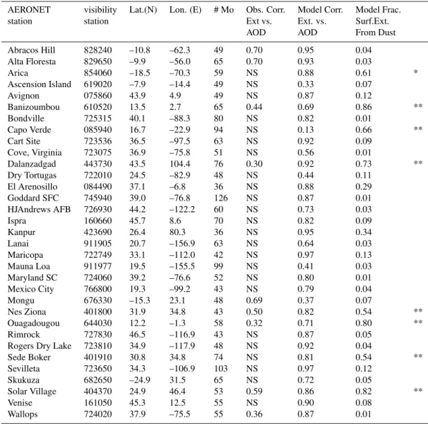
An-Table 1.Monthly mean AERONET aerosol optical depth vs. monthly mean surface extinction at closest meteorological station.
AERONET visibility Lat.(N) Lon. (E) # Mo Obs. Corr. Model Corr. Model Frac.
station station Ext vs. Ext. vs. Surf.Ext.
AOD AOD From Dust
Abracos Hill 828240 –10.8 –62.3 49 0.70 0.95 0.04
Alta Floresta 829650 –9.9 –56.0 65 0.70 0.93 0.03
Arica 854060 –18.5 –70.3 59 NS 0.88 0.61 *
Ascension Island 619020 –7.9 –14.4 49 NS 0.33 0.07
Avignon 075860 43.9 4.9 49 NS 0.87 0.12
Banizoumbou 610520 13.5 2.7 65 0.44 0.69 0.86 **
Bondville 725315 40.1 –88.3 80 NS 0.82 0.01
Capo Verde 085940 16.7 –22.9 94 NS 0.13 0.66 **
Cart Site 723536 36.5 –97.5 63 NS 0.92 0.09
Cove, Virginia 723075 36.9 –75.8 51 NS 0.56 0.01
Dalanzadgad 443730 43.5 104.4 76 0.30 0.92 0.73 **
Dry Tortugas 722010 24.5 –82.9 48 NS 0.44 0.11
El Arenosillo 084490 37.1 –6.8 36 NS 0.88 0.29
Goddard SFC 745940 39.0 –76.8 126 NS 0.87 0.01
HJAndrews AFB 726930 44.2 –122.2 60 NS 0.73 0.03
Ispra 160660 45.7 8.6 70 NS 0.82 0.09
Kanpur 423690 26.4 80.3 36 NS 0.95 0.34
Lanai 911905 20.7 –156.9 63 NS 0.64 0.03
Maricopa 722749 33.1 –112.0 42 NS 0.97 0.13
Mauna Loa 911977 19.5 –155.5 99 NS 0.41 0.03
Maryland SC 724060 39.2 –76.6 52 NS 0.80 0.01
Mexico City 766800 19.3 –99.2 43 NS 0.79 0.04
Mongu 676330 –15.3 23.1 48 0.69 0.37 0.07
Nes Ziona 401800 31.9 34.8 43 0.50 0.82 0.54 **
Ouagadougou 644030 12.2 –1.3 58 0.32 0.71 0.80 **
Rimrock 727830 46.5 –116.9 43 NS 0.87 0.05
Rogers Dry Lake 723810 34.9 –117.9 48 NS 0.92 0.04
Sede Boker 401910 30.8 34.8 74 NS 0.81 0.54 **
Sevilleta 723650 34.3 –106.9 103 NS 0.97 0.12
Skukuza 682650 –24.9 31.5 65 NS 0.72 0.05
Solar Village 404370 24.9 46.4 53 0.59 0.86 0.82 **
Venise 161050 45.3 12.5 55 NS 0.90 0.08
Wallops 724020 37.9 –75.5 55 0.36 0.87 0.01
NS indicates the correlation is not significant at the 99%.
* indicates that dust dominates other aerosols in the surface extinction and are included in the next Table. indicates that dust dominates other aerosols, but that fog is likely, so the station is omitted.
drews Air Force Base, where the closest visibility station is 1 degree away from the AERONET site.
For this paper we assume that the visibility data are of such a poor quality that it cannot be used as a proxy for dustiness until it has been verified that it shows aerosols seen in other reliable data. This is a different assumption than used in other studies, where the fraction of <1 km visibilty is assumed to be a reflection of dustiness (e.g. Kurosaki and Mikami, 2003). We think that until the data collection methods have much higher quality control, the measurement methods are better documented and an evaluation of the data occurs in the literature, we will not believe that visibility data contain quantatively interpretable value. Since that information is
not available, we are comparing the visibility data to data of known quality to better understand if the visibility data can be interpreted quantatively. Our goal is to understand what fraction of the visibility data can be interpreted as aerosols that are not just important at a very small scale, but impor-tant at a scale of 100+ km.
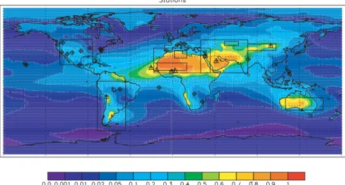
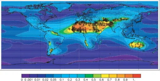
Fig. 1.Location of AERONET stations used in this analysis (diamonds and triangles). Triangles indicate stations where the surface extinction is dominated by dust, while diamonds are stations where other aerosols dominate (>50%) model predicted surface extinction (shown as colored contours), using the model of Rasch et al. (2001). Also shown are boxes outlining the different regions emphasized in the main text and following figures.
all the 33 stations across all time, which we will refer to as across all stations. This allows us to compare the visibility-derived variables over as large of a range of values as pos-sible. For most of the surface meteorological stations there is not a statistically significant correlation between AOD and any of the visibility-derived variables (e.g. Table 1, using the example of extinction). These low correlations could be be-cause surface extinction and column extinction (equivalent to AOD) are decoupled in these areas. The low correlations may be because of strong boundary layer inversions as an example. To test this hypothesis, we use model simulations (described in the methodology section) to correlate surface extinction and AOD in a model with the dominant aerosol types. The model suggests that at the locations in this com-parison, and over most of the globe, the surface extinction and AOD should be correlated at much higher levels than our results from the data (Fig. 2f and Table 1). Our model is a global model, so we could be missing small scale vari-ability that causes lower correlations in the data. In order to test for this possibility, we correlate the AERONET opti-cal depths from two nearby AERONET stations (Maryland Science Center vs. GSFC, see Table 1 for locations) with each other and we obtain a correlation coefficient of 0.99 suggesting that small scale variability in AOD is not likely to be causing all the discrepancy between the visibility data and column optical depth data in our variability comparisons. This suggests that neither surface extinction derived from the visibility data nor the fraction of observations with less than 1–10 km visibility are good indicators of regional aerosol op-tical depth at all stations. There are many possible explana-tions: the poor quality of the data; moisture impacts on the visibility through clouds; local dust sources (for example a
dirt road directly in front of the observer). On the other hand, this lack of correlation could also be that there are elevated aerosol layers which are not seen by the visibility measurer, but being observed by the AERONET data. At this point, we do not know which of these explanations are correct. Note that if we perform the correlation between monthly mean aerosol optical depth from AERONET and data from the visibility stations over all the stations, we obtain corre-lation coefficients of 0.30 and 0.34 for extinction and frac-tion of observafrac-tions with visiblity less than 5 km, respec-tively. We can obtain higher correlations across all stations using the fraction of observations less than 10 km (0.57), but this visibility-derived variable still has the high occurrence of non-statistically significant correlations at most stations, similar to that seen in Table 2 for extinction.
0 1 2 3 4
0 0.5 1 1.5 2
0 0.5 1 1.5 2
0 500 1000 1500 2000 2500 3000
0 0.5 1 1.5 2
0 500 1000 1500 2000 2500 3000
0 0.5 1 1.5 2 2.5 3 3.5
0 500 1000 1500 2000 2500 3000
0 0.5 1 1.5 2 2.5 3 3.5
0 500 1000 1500 2000 2500 3000
f. Aer. OD vs sfc ext r=0.85
A e r sf c e x t Aerosol OD a. b. c. d. e.
g. Dust sfc flux vs. dust sfc ext r=0.75 h. Dust sfc flux vs. aer. sfc ext r=0.69
j. Dust sfc flux vs. Aer OD r=0.38 i. Dust sfc flux vs dust OD r=0.46
Dust sfc flux (g/ m2/ year)
Dust sfc flux (g/ m2/ year)
Dust sfc flux (g/ m2/ year)
Dust sfc flux (g/ m2/ year)
D u st s fc e x t A e r. sf c e x t D u st O D A e r. O D
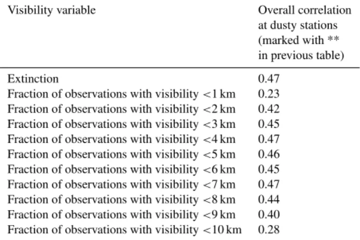
Table 2.Visibility proxies at dusty stations.
Visibility variable Overall correlation
at dusty stations (marked with ** in previous table)
Extinction 0.47
Fraction of observations with visibility<1 km 0.23
Fraction of observations with visibility<2 km 0.42
Fraction of observations with visibility<3 km 0.45
Fraction of observations with visibility<4 km 0.47
Fraction of observations with visibility<5 km 0.46
Fraction of observations with visibility<6 km 0.45
Fraction of observations with visibility<7 km 0.47
Fraction of observations with visibility<8 km 0.44
Fraction of observations with visibility<9 km 0.40
Fraction of observations with visibility<10 km 0.28
obtained (Table 2). The overall correlations for extinction and fraction of observations with a visibility<5 km are 0.47 and 0.46, respectively, indicating that about 22% of the vari-ability in the optical depths are captured in the visibility-derived variables. These correlation coefficients are not par-ticularly high, but using only the visibility at dusty stations, we are focusing on the stations with the highest correlations with aerosol optical depth.
We calculate the correlation with AERONET optical depth using a variety of visibility-derived variables in order to test which ones compare the best. We obtain the best correlations when we use visibility thresholds between 2–9 km, or use the extinction variable (Table 2), so we chose to continue our analysis with the 5 km threshold (VIS5) and the extinction variable (EXT). Notice that the fraction of events with vis-ibility less than 1 km does much worse than either of these two visibility proxies, although it has been previously used for dust studies (e.g. Kurosaki and Mikami., 2003). It is not clear why the 5 km threshold does better than 1 km thresh-olds in comparison with aerosol optical depth, but it could be because 1 km thresholds are more associated with highly localized events such as the location of a dirt road near the meteorological station.
In order to consider how well the visibility data compare to other datasets used for capturing variability, we repeat this analysis using the TOMS AAI and TOMS AOD – datasets with longer time periods than the AERONET data – that have been used to infer dust source variability (e.g. Mahowald et al., 2003a; Zender and Kwon, 2005). Using all AERONET sites, TOMS AAI and TOMS AOD have correlations of 0.65, 0.23, respectively, between the monthly mean values and AERONET optical depth. If we look only at dusty regions (again the stations marked with a ** in Table 1) TOMS AAI and TOMS AOD have correlations of 0.66 and 0.70, respec-tively. Thus, over dusty regions, TOMS AAI and TOMS
AOD have similar ability to capture variability in optical depths, but over other regions, TOMS AAI does better. This is not expected, since the AOD is constructed to better con-sider the effects of different aerosols. However, the TOMS AOD is a combination of model and data, and thus may be biased because of the model used to convert from an AAI to an AOD. There still may remain problems with the use of TOMS AAI or AOD because of drifts in the satellites when outside the 1984–1990 period where the AAI is most stable. 3.2 Theoretical value for inferring dust sources
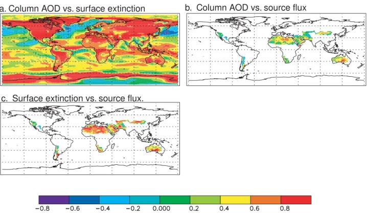
Now that we have evaluated the visibility data to indicate how good of a proxy it is for aerosol amount, we next con-sider what measurement is the best proxy for surface fluxes of dust. Visibility data are actually measures of surface ex-tinction. If this surface extinction comes solely from aerosols (and not from water vapor or clouds) it is linearly propor-tional to concentration. AOD is a measure of column ex-tinction. Neither of these variables is directly measuring the surface fluxes. Nonetheless, we are using either surface ex-tinction (visibility-derived variables) or AOD (e.g. Prospero et al., 2001) to try to gain information about surface fluxes. Here we test how much of the variability in surface fluxes is measured by variability in either surface extinctions or AOD. This is an example of a problem where model calculations can provide great insight into how to best infer spatial and temporal variability in surface fluxes when we have no direct measurements. When we try to estimate variability in surface dust fluxes based on other measurements, previous model analyses have suggested that dust surface concentration will capture the variability better than dust column amount (Ma-howald et al., 2003b). We extend that analysis here to corre-late modeled total aerosol (sum of sulphate, carbonaceous, dust and seasalt) AOD with modeled surface dust fluxes. In the real world, we do not have data directly measuring dust source fluxes, so we will use the aforementioned model to estimate the relationship between variables we can mea-sure (surface extinction or column amount) and dust fluxes (Sect. 3.2). Errors in the model formulation of boundary layer mixing or ventilation, or horizontal transport will cause errors in this correlation. In addition, AERONET includes only cloud free days, while we include all days, causing a possible discrepancy. However, no other methods have been postulated to evaluate the ability of different measurements of dust concentration or optical depth to infer information about dust flux spatial or temporal variability.
c. Surface extinction vs. source flux.
b. Column AOD vs. source flux
a. Column AOD vs. surface extinction
Fig. 3.Correlations of monthly mean modeled column aerosol optical depth (AOD) versus surface extinction(a), AOD vs. surface fluxes(b)
and surface extinction vs. surface fluxes(c).
appear more related to surface fluxes than optical depth vi-sually. This is very clear in the scatter plots or the correla-tion coefficients, which are shown for all land grid points in the model. The correlation coefficients between the spatial locations of dust surface fluxes and surface extinction or op-tical depth in model are 0.75 and 0.46, respectively. Since in the real world, we have total aerosol optical depth, not just dust optical depth, that we are using to infer the dust source variability, we can correlate those values instead in a model. Correlating total aerosol and dust surface fluxes results in correlation coefficients of 0.69 and 0.38, corresponding to capturing 48% or 14%, respectively, of the spatial variabil-ity in dust surface fluxes, when we use surface extinction or optical depths, respectively. In the real world we only have visibility data at a limited number of stations, not globally as we do in the model. If we sample the model output at these stations only, our correlation coefficient between extinction and dust fluxes does not change substantially (0.73). How-ever, this correlation does not include the effect of the low spatial resolution of the visibility data, especially in desert areas. In the real world, TOMS AAI does not sample optical depth, but an aerosol index which is linearly proportional to altitude, making it likely to perform worse at detecting dust source fluxes than the model estimates here. The strength of sources is not well related to the frequency of emissions (Laurent et al., 2005), suggesting that sampling the number of times TOMS AAI is above a certain threshold (e.g.
Pros-pero et al., 2002) is not necessarily a better way to obtain information about the sources. (Notice that for our visibility-derived variable, VIS5, which is a frequency variable, does about as well as the EXT variable.) Thus, visibility-derived variables should theoretically do a better job of capturing the spatial variability in dust fluxes than satellite derived optical depth. Whether they practically do is based on their ability to capture regional scale aerosol fluctuations, which is exam-ined in detail in Sect. 3.1.
Fig 4. Location of visibility stations
Fig. 4.Location of visibility stations with more than 30 years of data. Colored contours show fraction of surface extinction from desert dust. Pluses show stations in regions dominated by desert dust (>50%), while dots show other locations.
may be poorly correlated for many reasons that are quite le-gitimate (e.g. TOMS AAI measures absorbing aerosols, not total aerosols). Although previous studies have implicitly as-sumed that satellite derived aerosol optical depths provide more information about spatial and temporal variability in dust sources than visibility measurements (e.g. Goudie and Middleton, 2001; Prospero et al., 2002) this analysis does not clearly support that assumption.
4 Visibility trends and correlations in dust regions
Since the analysis in Sect. 3 indicates that visibility best correlates with aerosol optical depth in dust dominated re-gions, we focus on the visibility-derived measures of dust here. Dust dominated regions are defined as those regions where dust contributes to at least 50% of the surface aerosol extinction in model simulations (Rasch et al., 2001). Fig-ure 4 shows the locations of meteorological stations with at least 30 years of data, and those within our dust dominated region. There are 357 stations from dust dominated regions included in the analysis of the visibility data. We analyze these stations grouped together by region, as well as individ-ually. For this analysis, we focus on annual means and an-nual mean correlations for simplicity of presentation. Quali-tatively similar results were obtained when monthly anoma-lies were used.
The mean fraction of observations when visibility is less than 5 km (VIS5) and mean surface extinction (EXT) derived from visibility are shown in Fig. 5 averaged over the pe-riod of 1974–2003. If we interpret this map as a proxy for dustiness, it gives us a very different view of where the dust sources are than what we get from TOMS AAI (e.g. Prospero et al., 2002). The Bodele basin does not appear to be the largest source of dust in this region, as some have claimed
(e.g. Prospero et al., 2002), and looks quite moderate in this dataset. In our model, which has a strong source of dust in the Bodele basin (seen in Fig. 2b), the model overpre-dicts the surface extinction downwind of the Bodele basin (relatively speaking–the values can not be compared quan-tatively), and the visibility stations do appear to be down-wind of the Bodele basin plume. One area that stands out in this analysis as having low visibility (high VIS5 and EXT) is the region around Pakistan and India, with low visibil-ity also seen in parts of North Africa, the Middle East and China/Mongolia. We normally do not think of the region near Pakistan and northwestern India as being the largest dust source (e.g. Goudie and Middleton, 2001; Prospero et al., 2002), and the reason this region has such high VIS5 and EXT values could be due to anthropogenic aerosols that may be stronger than our model predicts. On the other hand, Pakistan and northwestern India is generally a highly popu-lated region with an arid climate, and with some of the high-est rates of reported desertification (Middleton and Thomas, 1997), so the visibility data could be correct. It is also pos-sible that the visibility data are biased in that a given station could stop reporting data during dust events, biasing where the visibility data suggests the most aerosols are located. There are no stations in North America where dust repre-sents 50% of the surface extinction, and the stations in South Africa are too few to include for a conclusive analysis. The global distribution of EXT (extinction) and VIS5 (fraction of observations with visibility less than 5 km) is different, and this is one of the reasons we analyze both variables. They are equally good (or bad) measures of aerosol optical depth, according to Sect. 3, and yet they are measuring aerosols dif-ferently – the number of extreme events (VIS5) compared to background visibility plus extreme events (EXT).
a. VIS5
b. EXT
c. VIS1
d. Blowing dust or sand
North Africa
a.
b.
c.
d.
e.
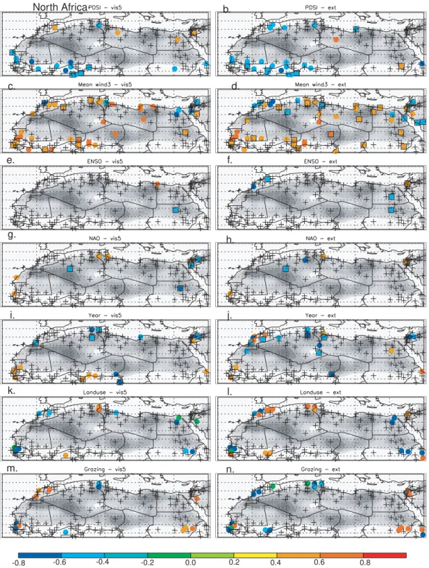
Fig. 6.Time series of the annual average over all the North Africa stations for extinction (EXT), fraction of visibility<5 km (VIS5), mean of the cube of the winds, median winds cubed, precipitation, Palmer Drought Severity Index (PDSI), percent of area under cultivation, percent of area under grazing, number of observations and number of stations included in the averages for each year. Figures 1 and 7 show the region over which the stations are averaged. Variable described on the left axis is in black and on the right axis is in blue.
globally in Fig. 1. For North Africa, we show a time series of the average visibility, winds, precipitation, Palmer drought severity index (PDSI) and human land use and grazing in Fig. 6. These values are averaged over the station locations (not over the entire region), to weight them in a manner similar to the visibility. Note that the data at neighboring stations should not be considered statistically independent. Visibility-derived variables (both EXT and VIS5) appear to vary substantially over the time series, even averaged over the whole of North Africa. We can see many visibility events and high extinction during the 1970–1980s, associated with the Sahel drought and higher downwind dust concentrations (e.g. Prospero and Nees, 1986; Prospero and Lamb, 2003). After the 1980s, fractions of VIS5 values decrease by about 50% while the extinction values decrease more slowly. There is a peak of low visibility during the 1950s associated with high winds, but the data are quite spotty during the 1940– 1960s. Thus it is not clear how robust these changes are (the standard deviations are large relative to the signals, not shown), although they appear at several different stations (not shown). Precipitation varies over this time period, domi-nated by the Sahel drought signal, and the Palmer drought severity index (PDSI) is highly correlated with precipitation
(Dai et al., 2004). Cultivation tends to be increasing over this time period, while grazing is decreasing, especially after the 1950s. The poor temporal resolution of observations re-lated to land use is obvious from this figure. Data availability is highly variable over the time period with most consistent observations only available after 1974. This is true in all of dust regions, and because of this we focus our analysis on the period 1974–2003.
b.
c. d.
North Africa.
e. f.
g.
h.
i. j.
k. l.
m. n.
-0.8 -0.6 -0.4 -0.2 0.0 0.2 0.4 0.6 0.8
Algeria
a.
b.
c.
d.
e.
Fig. 8.Same as Fig. 6, but for a region around Algeria (28 N to 3 N, 2 E to 15 E and shown in Fig. 1).
correlations are between the PDSI and mean cube of the winds and the VIS5 or EXT variable. We use mean cube of the winds because the strength of dust sources is usually proportional to winds cubed (e.g. Mahowald et al., 2005). This suggests that meteorology drives most of the temporal variability in North Africa, consistent with previous studies (e.g. Prospero and Nees, 1986; N’Tchayi Mbourou et al., 1997; Prospero and Lamb, 2003). The correlations at most stations between PDSI and visibility tend to be larger in mag-nitude than between precipitation, previous year’s precipita-tion or the previous year’s PDSI and visibility (not shown), consistent with drought severity being a better measure of soil moisture than precipitation alone. Thus, we focus on us-ing the PDSI for the rest of the analyses. There is little cor-relation between ENSO or NAO (Trenberth and Stepaniak, 2001; Hurrell, 1995) and visibility in North Africa (similar to Moulin and Chiapelo, 2004; Chiapelo et al., 2005), un-like further downwind using other datasets (e.g. Moulin et al., 1997; Mahowald et al., 2003b). There are some statisti-cally significant trends in time (i.e. correlations with year) in the VIS5 and EXT, although they are opposite in sign in some cases along the Mediterranean coast of North Africa, indicat-ing that the number of events is goindicat-ing up, but the background aerosol concentration may be going down. If we calculate the correlation over 1940–2003, instead of just over the time period between 1974 and 2003, we obtain much stronger correlations between year and extinction and between land
use and extinction along the Mediterranean coast of North Africa, perhaps associated with the difference in the amount of data. Figure 8 shows the average time series in a region centered on Algeria (28 N to 3 N, 2 E to 15 E). This shows that there is little data before 1974, but that the data suggest episodes of high VIS5 and EXT during the 1950s and 1960s. There is a tendency for EXT to be higher later in the cen-tury, consistent with a correlation between EXT and year at individual stations (not just because of discontinuities in data records at individual stations). There is also a positive corre-lation between EXT and cropland and a negative correcorre-lation between EXT and grazing (since cropland and grazing are almost linearly increasing and decreasing, respectively, over the 1940–1990s). Similar behaviour is seen for the average of all the stations in the W. Sahel (13 N to 22 N, 20 W to 15 E) time series (Fig. 9), with a peak in VIS5 and EXT in 1985 (during the Sahel drought), with some high values of VIS5 and EXT in the 1940s and 1950s.
West Sahel
a.
b.
c.
e.
f.
Fig. 9.Same as Fig. 6, but for a region in the Western Sahel (13 N to 22 N, 20 W to 15 E also shown in Fig. 1).
Middle East
a.
b.
c.
e.
e.
a. Middle East b.
c. d.
e. f.
g. h.
i. j.
-0.8 -0.6 -0.4 -0.2 0.0 0.2 0.4 0.6 0.8
Fig. 11. Same as Fig. 6, but for the Middle East (ENSO and NAO are not included).
as in North Africa, but that there are statistically significant temporal trends. There are also correlations between human activities (cropland or grazing) and dust in different parts of the Middle East. There are statistically significant decreases in Pakistan/India over 1974–2003. If we look at correlations in Pakistsan/India over the longer time period (back to the
1940s) there are more stations with positive trends in VIS5 and EXT (not shown) and more statistically significant cor-relations with cropland and grazing (both positive and nega-tive).
China
a.
b.
c.
d.
e.
Fig. 12.Same as Fig. 6, but for a region near China (region shown in Fig. 13).
similar to other regions, and a downward trend between 1974 and 2003 (Fig. 12). Correlations between VIS5 and EXT and other variables (Fig. 13) suggest that precipitation is not im-portant for variability in visibility, but that winds are cor-related with variability in visibility, similar to the results seen in other studies (e.g. Zhang et al., 2003; Sun et al., 2001; Zhao et al., 2004; Liu et al., 2004). Our data do not show the increase in dustiness in 2000-2002 seen in Kurosaki and Mikami (2003), although our results are consistent with their conclusion that wind drives variability in dust events. Kurosaki and Mikami (2003) include in their analysis many stations close to urban areas in China, which are excluded in our analysis.
For Australia, there are fewer stations compared to the other regions previously discussed, but again we see the low visibility in the 1950s (with large standard deviations, not shown), with less variability between 1974 and 2003 in the VIS5 and EXT data. There is an exception in the year 1986, which is anomalously high, especially for VIS5 (Fig. 14). Correlations at specific stations (Fig. 15) suggest that PDSI has the strongest correlations with dust, but in a manner that is counterintuitive – the higher the water availability is, the more dust. This makes some sense as a dust correlation if the increasing water makes the soil more erodible because the water brings more erodible sediment into the dry fluvial channels and lake beds or breaks up crusts (e.g. Okin and Reheis, 2002; Mahowald et al., 2003a; Zender and Kwon,
2005. But this counterintuitive correlation could also be due to other aerosols or increasing water vapor changing visibil-ity as well. There are downward trends in VIS5 and EXT over the 1974–2003 time periods at some stations (similar results are seen for Fig. 15 when the whole time period is considered). There are 2 (out of 16) stations with statisti-cally significant correlations between VIS5 and ENSO, but these significant correlations are not matched between EXT and ENSO. (* This is in contrast to the correlation between El Nino and precipitation in many regions of Australia, al-though not necessarily across the dust region (Dai et al., 1998).
In South America, there are 7 stations with data for part of the time period. Again there are low visibilities at the first part of the time series, and then flatter visibility trends for the rest of the time series (Fig. 16). There are few correla-tions between the station data and other variables (Fig. 17). Some stations indicate that wind speeds are anti-correlated with VIS5 and EXT (which may indicate that these stations are not dust dominated and should be ignored), and there are some correlations between year, cropland, grazing and pre-cipitation, but no large scale patterns. Only one station has a correlation between ENSO and EXT.
a. China b.
c. d.
e. f.
g. h.
i. j.
-0.8 -0.6 -0.4 -0.2 0.0 0.2 0.4 0.6 0.8
Fig. 13.Same as Fig. 11, but for a region near China.
of data. First we look at the Southwestern U.S. region (e.g. Prospero et al., 2001) (Fig. 19 shows the region). A time series plot shows that both VIS5 and EXT have been roughly increasing since the 1940s, with a lot of variability (Fig. 18). For this region, the data are more regularly available prior to 1974 than in previous regions, so we show correlations from 1940 to 2003 (Fig. 19). There are statistically significant cor-relations between most of the variables and VIS5 or EXT.
Australia
a.
b.
c.
d.
e
Fig. 14.Same as Fig. 6, but for a region in Australia (region shown in Fig. 15).
Table 3.Correlation coefficients with time and visibility-derived variables. If a significant correlation exists, this implies a trend with time. Only values significant at the 95% are shown here.
Region EXT correlation with time VIS5 correlation with time 1974–2003 (whole time)
All dusty regions NS (NS) NS (NS)
N. Africa NS (0.79) NS (0.43)
Middle East 0.40 (0.42) 0.57 (0.35)
China –0.86 (–0.59) –0.89 (–0.72)
Australia NS (NS) NS (–0.30)
South America NS (–0.22) 0.39 (–0.40)
these results difficult, and are consistent with the results of the model suggesting that visibility in this region is not dom-inated by dust.
The Aral Sea area is another region which is thought to have a great deal of dust (e.g. Prospero et al., 2001), although our model does not predict dust as the dominant source of surface extinction. VIS5 and EXT tended to be high during the 1950s, and are lower now (Fig. 20). Similarly, winds were higher in the 1950s than today. These might be indi-cations that the data quality or location of the measurement devices have changed, or it could be an indication that there are real changes in the conditions in the Aral Sea. Similar to North America, the amount of data is relatively stable over
a. Australia b.
c. d.
e. f.
g. h.
i. j.
-0.8 -0.6 -0.4 -0.2 0.0 0.2 0.4 0.6 0.8
Fig. 15.Same as Fig. 11, but for a region near Australia.
If we consider the average of all 357 stations in dusty re-gions (Fig. 22), we see that the 1940s and 1950s were periods with relatively high VIS5 and EXT. These were more windy periods, although there is also more variability in winds. It is interesting that there was higher VIS5 and EXT during this period, but it raises a question about the data. It could be that during this period, there were more dirt roads close to the meteorological stations, and this caused lower
South America
a.
b.
c.
d.
e.
Fig. 16.Same as for Fig. 6, but for a region in South America (shown in Fig. 17).
suspicious. Thus, we may want to readdress previous stud-ies which have suggested the 1950s were dustier in China than current (Zijiang and Guocai, 2003), as an example, and see if there are independent datasets which allow us to check that this result is not because of biases in the data collection method. On the other hand, it is possible that the 1940s and 1950s were a much dustier time period in all dust regions globally. Over the whole time period, there is no statisti-cally significant trend in EXT or VIS5 for all regions taken together. For some regions (China, Middle East or South America) there are statistically significant trends with time in the visibility-derived variables over the whole time period or 1974–2003 (see Table 3).
Another way to analyze the same data is to look at corre-lations between VIS5 and EXT and other variables not over time, but in space across the stations. If we look at the spatial correlations across all regions using the means over all years (or over 1974–2003, the results do not change qualitatively), we can look at some different hypotheses about drivers of dust variability spatially. For the correlations between visi-bility parameters and topographic lows we use three repre-sentations: the preferential source distribution of Ginoux et al. (2001), the dust source used in the NCAR Community Atmospheric Model (Mahowald et al., 2006) (which is based on the Zender et al. (2003b) geomorphic soil erodibility fac-tor which calculates upstream area and satellite derived
a. S. America b.
c. d.
e. f.
g. h.
i. j.
-0.8 -0.6 -0.4 -0.2 0.0 0.2 0.4 0.6 0.8
Fig. 17.Same as for Fig. 11, but for a region near South America.
If we include winds cubed, PDSI, croplands, grazing and to-pographic lows, slightly higher correlations coefficients are found than for any individual process (0.58 and 0.50 vs. 0.55 and 0.45 for VIS5 and EXT, respectively), and these results also suggest that cultivation is the most reliable variable for predicting visibility distributions. This result is consistent with the view of visibility that we obtain from Fig. 5, where the lowest visibility (i.e. highest VIS5 and EXT) is observed
a.
b.
c.
d.
e.
North America (non-dust dominated)
Fig. 18.Same as for Fig. 6, but for a region in North America (shown in Fig. 19 and Fig. 1). This region is one where the model predicts that dust does not dominate the aerosol extinction in the surface layer.
Table 4.Spatial correlations between visibility-derived variables and other variables (values not significant at the 99% are indicated by NS; NA indicates no data).
Variable VIS5 EXT VIS1 Blowing dust
Mean winds cubed NS NS NS NA
Median winds –0.27 –0.21 NS NA
Precipitation NS NS NS –0.39
PDSI NS NS NS NS
Cultivation (Ramankutty 0.55 0.45 NS NS and Foley, 1998)
Cultivation (Ramankutty, 0.48 0.41 NS NS personal communication)
Grazing NS NS NS NS
Topographic low NS NS NS 0.31
(Ginoux et al., 2001)
Topographic Low NS NS NS 0.41
(upstream area) (Zender et al., 2003b)
Topographic low NS NS NS 0.46
(surface reflectance) (Grini et al., 2004)
These results are sensitive to which variable we use. If we use the fraction of visibility less than 1km (also shown in Fig. 4 and Table 4), we obtain no statistically
a. N. America b.
c. d.
e. f.
g. h.
i. j.
-0.8 -0.6 -0.4 -0.2 0.0 0.2 0.4 0.6 0.8
Fig. 19.Same as Fig. 11, but for a region in North America.
of I. Tegen and S. Engelstaedter), we obtain similar results to those obtained in that study (Fig. 4 and Table 4) – the dustiness in this dataset is correlated with natural dry lake beds, and not with land use proxies. In doing this compar-ison, we realized that the dust storm frequency dataset used
Aral Sea
a.
b.
c.
d.
e.
Fig. 20. Same as Fig. 6, but for a region near the Aral Sea (shown in Fig. 20 and Fig. 1). This region is one where the model predicts that dust does not dominate the aerosol extinction in the surface layer.
However, interpreting the dust storm frequency dataset used in Engelstaedter et al. (2003) as blowing dust or sand makes this dataset consistent with the results of this and other pre-vious studies which analyzed data at particular stations (e.g. N’Tchayi Mbourou et al., 1997).
We do not know which of these variables best represent the true location of the dust sources, since we do not know where the sources are. Here, we emphasize the results based on the VIS5 and EXT visibility-derived variables, since we are able to correlate them with a known quantatity (AERONET aerosol optical depth in Sect. 3.1), and we think that the frac-tion of the VIS5 or EXT that correlates with the AERONET aerosol optical depth represents “regional” aerosols, not a very local source.
5 Summary and conclusions
This study focuses on using visibility data from surface me-teorological stations as an indicator of dust variability, and specifically dust source variability. Because the quantitative nature of visibility data is not well established, we first eval-uate the utility visibility data for our purposes. Our goal is to look at long term variability, so we use the monthly mean AERONET aerosol optical depth (AOD) at the 33 stations with more than 3 years of data. While AERONET data are
high quality, it is not available as spatially or temporally ex-tensively as the visibility data.
a. Aral Sea b.
c. d.
e. f.
g. h.
i. j.
-0.8 -0.6 -0.4 -0.2 0.0 0.2 0.4 0.6 0.8
Fig. 21.Same as Fig. 11, but for a region near the Aral Sea.
those variables for most of the analyses in this paper. The fraction of observations with visibility less than 1 km may be indicative of some other important value, but we do not know how to evaluate its accuracy.
Similar correlation analyses using the TOMS AAI and TOMS AOD data suggest that they are able to capture about 45–49% of the variability in the AERONET optical depth data over dusty regions (correlation coefficients of 0.67 and
0.7). Note that the TOMS AOD only has a correlation coef-ficient of 0.23 over all AERONET stations, suggesting that it is not a robust measure of temporally and spatial variability in aerosol optical depth in non-dusty regions, even ignoring problems in satellite drift outside the 1984–1990 period.
All dusty stations
a.
b.
c.
d.
e.
Fig. 22.Same as Fig. 6, but for an average across all the dusty stations considered in this study.
since we cannot directly measure dust source surface fluxes globally. Using models we can better understand which vari-ables best represent the spatial and temporal variability in dust source surface fluxes. Our calculations show that face extinction should be much better related to source sur-face fluxes of dust than column amount (correlation coeffi-cient of 0.73 vs. 0.38, equals 36% vs. 10% of variability, re-spectively). However, the visibility data has problems with its quality. Thus, it is unclear whether satellite aerosol opti-cal depth or visibility-derived variability best gives informa-tion about variability in dust sources (either spatial or tem-poral). Some studies assume that TOMS AAI represents the long-range transported dust (e.g. Prospero et al., 2002). Be-cause TOMS AAI is linearly proportional to the height of the dust, this is probably true (Torres et al., 1998; Mahowald and Dufresne, 2004). However, this also makes TOMS AAI less appropriate for studying spatial or temporal variability in dust source fluxes. The visibility-derived-proxies repre-sent regional aerosols to the extent that they correlate with the AERONET AODs, and thus represent dust that has been transported somewhere from the kilometer to the hundreds of kilometers scale. The analysis here suggests that visibility data and TOMS AAI or TOMS AOD may be equivalently good (or bad) at representing the spatial and temporal vari-ability in surface dust fluxes. Indeed, from their characteris-tics, TOMS AAI will get higher altitude dust while visibil-ity data will see dust confined to close to the surface. More
work on determining better ways to determine the location of dust source areas is vital, since the two main datasets we have to address dust sources (satellite optical depths or vis-ibility data) show different results. We examined the tem-poral trends in VIS5 and EXT in regions dominated by dust, where the visibility-derived variables are able to capture over 20% of the variability in aerosol optical depth measured by AERONET. Although meteorological station data are avail-able from 1900 to 2003, in dusty regions there are only data after 1940 in our dataset. The data record prior to 1974 is not consistent, forcing us to limit our analysis of “long” term trends to the last 30 years. This is disappointing, since we had hoped to extend the satellite record significantly into the pre-1980s period. This implies we are missing any processes occurring prior to the 1970s.
There are a relatively stable number of observations after 1974 in the dataset over dusty regions, so we conducted most of our correlation analyses between individual station time series of VIS5 or EXT and other variables during the pe-riod 1974–2003. For analysis we present simple and more commonly used correlation coefficients, but rank correla-tions show qualitatively similar results. However, in many cases, there are multiple variables which correlate with the visibility-derived proxies, making it more difficult to inter-pret the results. We focus on results that are regionally co-herent. The high correlation coefficients between annually averaged PDSI and both VIS5 and EXT are consistent with precipitation being very important in the Sahel region of North Africa and the Mediterranean coast of North Africa. High correlations between winds and VIS5 or EXT in China are consistent with winds driving much of the variability of dustiness in China. In other regions, the correlation coef-ficients are not statistically significant on a regional basis. In no region are there large numbers of strong correlations between either NAO or ENSO and visibility, unlike what is seen farther downwind (e.g. Moulin et al., 1997; Mahowald et al., 2003b; Prospero and Lamb, 2003; Moulin and Chia-pello, 2004). Temporally, correlations between human culti-vation or grazing and visibility-derived variables are not seen over large regions in our datasets, perhaps due to the poor temporal quality of the cultivation and grazing datasets.
There are regions with statistically significant trends with time in VIS5 or EXT for the period 1974–2003 (seen as a correlation between year and these variables). Upward trends with time are seen regionally in parts of North Africa, espe-cially in EXT, correlated with lower precipitation. Down-ward trends are seen in regionally broader areas, including parts of Central Asia and China. Looking at the average across all 357 stations in dusty regions, there is no statisti-cally significant trend in VIS5 or EXT. Note that analyses of North America and the region close to Aral Sea (while more uncertain because these regions’ visibility is not dominated by mineral aerosols) suggest that EXT and VIS5 are decreas-ing in these regions.
We get a different picture of the important processes if we look spatially across stations instead of at individual stations over time. The hypothesis that dry lake beds are dust sources is not supported, since there is no significant correlation be-tween mean VIS5 or EXT in our data and three measures of the topographic lows (to the extent that topographic lows rep-resent dry lakebeds). Instead the most consistent correlations are between VIS5 and EXT and cultivation across all regions, with correlation coefficients suggesting that approximately 30% of the spatial distribution in the dustiness in the stations is associated with cultivation (note this does not mean that the cultivation source of dust is 30% of the dust flux, because of the statistics used here). Most of this cultivation related dusti-ness appears to be in the Pakistan/India region (see Fig. 5). This may indicate that the results here may be sensitive to the quality of this data as a reflection of dust sources. We may be
seeing a different signal in the spatial versus temporal anal-ysis because most of the dust sources may have been gener-ated prior to 1974 in the cultivgener-ated regions. To add complex-ity to this isue, if we use a different meteorological dataset based on blowing dust or sand (as used in Engelstaedter et al., 2003), dry lake beds or topographic lows are consistent with the data (correlation coefficients between 0.3 and 0.46), but cultivation is not.
perturbations may control where some of the dust sources are, but that meteorological variability controls the temporal variability over the last 30 years. However, the potential bi-ases of the visibility dataset prevent strong conclusions based solely on these results.
Acknowledgements. The authors thank A. Dai, C. Zender and
P. Rasch for datasets used in this analysis. We would like to thank the AERONET, TOMS AAI and TOMS AOD principal investigators for making available data. We would like to thank C. Zender, R. Miller, S. Engelstaedter and I Tegen for comments on the text.
Edited by: F. J. Dentener
References
Baker, J., Southhard, R., and Mitchell, J.: Agricultural dust pro-duction in standard and conservation tillage systems in the San Joaquin Valley, J. Environ. Qual., 34, 1260–1269, 2006. Baker, J., Ballantine, J.-A. C., Okin, G. S., Prentiss, D. E., and
Roberts, D. A.: Mapping landforms in North Africa using conti-nental scale unmixing of MODIS imagery, Rem. Sens. Environ., 97, 470–483, 2005.
Bonan, G., Levis, S., Kergoat, L., and Oleson, K.: Landscapes as patches of plant functional types: An integrating concept for cli-mate and ecosystem models, Global Biogeochem. Cy., 16, 5.1– 5.23, 2002.
Chen, M., Xie, P., Janowiak, J., and Arkin, P.: Global land precipi-tation: a 50-year monthly analysis based on gauge observations, J. Hydrometeorol., 3, 249–266, 2002.
Chiapello, I., Moulin, C., and Prospero, J.: Understanding the long-term variability of African dust transport across the At-lantic as recorrded in both Barbados surface concentrations and large scales TOMS optical thicknesses, J. Geophys. Res., 110, D18S10, doi:10.1029/2004JD005132, 2005.
Dai, A., Fung, I. Y., and Del Genio, A. D.: Surface observed global land precipitation variations during 1900–88, J. Climate, 10, 2943–2962, 1997.
Dai, A., Trenberth, K. E., and Karl, T. R.: Global Variations in Droughts and Wet Spells, Geophys. Res. Lett., 25, 3367–3370, 1998.
Dai, A., Trenberth, K., and Qian, T.: A global dataset of Palmer Drought Severity Index for 1870–2002: Relationship with soil moisture and the effects of surface warming, J. Hydrometeorol., 5, 1117–1130, 2004.
DeMott, P., Sassen, K., Poellot, M., et al.: African dust aerosols as atmospheric ice nuclei, Geophys. Res. Lett., 30, 1732, doi:10.1029/2003GL017410, 2003.
Dentener, F. J., Carmichael, G. R., Zhang, Y., Lelieveld, J., and Crutzen, P. J.: Role of mineral aerosol as a reactive surface in the global troposphere, J. Geophys. Res., 101, 22 869–22 889, 1996. Engelstaedter, S., Kohfeld, K. E., Tegen, I., and Harrison, S. P.: Controls of dust emissions by vegetation and topographic depres-sions: An evaluation using dust storm frequency data, Geophys. Res. Lett., 30, 1294, doi:10.1029/2002GL016471, 2003. Gillette, D. A.: Threshold friction velocities for dust production for
agricultural soils, J. Geophys. Res., 93, 12 645–12 662, 1988.
Ginoux, P. Chin, M., Tegen, I., et al.: Sources and distribution of dust aerosols with the GOCART model, J. Geophys. Res., 106, 20 255–20 273, 2001.
Godish, T.: Air Quality. CRC Press, Boca Raton, Florida, 1997. Goudie, A. and Middleton, N.: Saharan dust storms: nature and
consequences, Earth-Sci. Rev., 56, 179–204, 2001.
Goudie, A. S. and Middleton, N. J.: The Changing Frequency of Dust Storms Through Time, Climatic Change, 20, 197–225, 1992.
Grini, A. and Zender, C.: Roles of saltation, sandblasting, and wind speed variability on mineral dust aerosol size distribution during the Puerto Rican Dust Experiment (PRIDE), J. Geophys. Res., 109, D07202, doi:10.1029/2003JD004233, 2004.
Holben, B. N., Eck, T., Slutsker, I., et al.: AERONET-A Federated Instrument Network and Data Archeive for Aerosol Characteri-zation, 2000.
Holben, B. N., Tanre, D., Smirnov, A. et al.: An emerging ground-based aerosol climatology:Aerosol optical depth from AERONET, J. Geophys. Res., 106, 12 067–12 097, 2001. Hurrell, J. W.: Decadal Trends in the North Atlantic Oscillation
Re-gional Temperatures and Precipitation, Science, 269, 676–679, 1995.
Jickells, T., An, Z., Anderson, K., et al.: Global iron connections between dust, ocean biogeochemistry and climate, Science, 308, 67–71, 2005.
Kistler, R., Kalnay, E., Collins, W., et al.: The NCEP-NCAR 50-Year Reanalysis: Monthly Means CD-ROM and Documentation, B. Am. Meteorol. Soc., 82, 247–267, 2001.
Klein-Goldewijk, K.: Estimating global land use change over the past 300 years: the HYDE database, Global Biogeochem. Cy., 15, 417–434, 2001.
Kurosaki, Y. and Mikami, M.: Recent frequent dust events and their relation to surface wind in East Asia, Geophys. Res. Lett., 30, 1736, doi:10.1029/2003GL017261, 2003.
Laurent, B., Maricorena, B., Bergametti, G., Chazette, P., Maig-nan, F., and Schmetig, C.: Simulation of the mineral dust emis-sion frequencies from desert areas of China and Mongolia us-ing an aerodynamic roughness length map derived from the POLDER/ADEOS 1 surface products, J. Geophys. Res., 110, D18S04, doi:10.1029/2004JD005013, 2005.
Liu, X., Yin, Z.-Y., Zhang, X., and Yang, X.: Analyses of the spring dust storm frequency of northern China in relation to antecedent and concurrent wind, precipitation, vegetation and soil moisture conditions, J. Geophys. Res., 109, D16210, doi:10.1029/2004JD004615, 2004.
Luo, C., Mahowald, N., and Corral, J. D.: Sensitivity study of meteorological parameters on mineral aerosol mobiliza-tion, transport and idstribumobiliza-tion, J. Geophys. Res., 108, 4447, doi:10.1029/2003JD0003483, 2003.
Mahowald, N., Baker, A., Bergametti, G., et al.: The atmospheric global dust cycle and iron inputs to the ocean, Global Bio-geochem. Cy., 19, GB4025, doi:10.1029/2004GB002402, 2005. Mahowald, N., Bryant, R., Corral, J. D., and Steinberger, L.: Ephemeral lakes and desert dust sources, Geophys. Res. Lett., 30, 1074, doi:10.1029/2002GL016041, 2003a.