Time series analysis of water surface temperature and heat flux
components in the Itumbiara Reservoir (GO), Brazil
Análise da série temporal da temperatura da superfície da água e dos componentes do
balanço de calor no Reservatório de Itumbiara (GO), Brasil
Enner Herenio de Alcântara, José Luiz Stech, João Antônio LorenzzettiandEvlyn Márcia Leão de Moraes Novo
Brazilian Institute for Space Research, Remote Sensing Division, CEP 12227-010, São José dos Campos, SP, Brazil
e-mail: [email protected]; [email protected]; [email protected]; [email protected]
Abstract: Aim: Water temperature plays an important role in ecological functioning and in controlling the biogeochemical processes of the aquatic system. Conventional water quality monitoring is expensive and time consuming. It is particularly challenging for large water bodies. Conversely, remote sensing can be considered a powerful tool to assess important properties of aquatic systems because it provides synoptic and frequent data acquisition over large areas. The objective of this study was to analyze time series of surface water temperature and heat flux to advance the understanding of temporal variations in a hydroelectric reservoir. Method: MODIS water-surface temperature (WST) level 2, 1 km nominal resolution data (MOD11L2, version 5) were used. All available clear-sky MODIS/Terra images from 2003 to 2008 were used, resulting in a total of 786 daytime and 473 nighttime images. Time series of surface water temperature was obtained computing the monthly mean in a 3 × 3 window of three reservoir selected sites: 1) near the dam, 2) at the centre of the reservoir and 3) in the confluence of the rivers. In-situ meteorological data from 2003 to 2008 were used to calculate surface energy budget time series. Cross-wavelet, coherence and phase analysis were carried out to compute the correlation between daytime and nighttime surface water temperatures and the computed heat fluxes. Results: The monthly mean of the day-time WST shows lager variability than the night-time WST. All time series (daytime and nighttime) have a cyclical pattern, passing for a minimum (June - July) and a maximum (December and January). Fourier and the Wavelet Analysis were applied to analyze this cyclical pattern. The daytime time series, presents peaks in 4.5, 6 12 and 36 months and the nighttime WST shows the highest spectral density at 12, 6, 3 and 2 months. The multiple regression analysis shows that for daytime WST, the heat flux terms explain 89% of the annual variation (RMS = 0.89 °C, p < 0.0013). For nighttime, the heat flux terms explain 94% (RMS = 0.53 °C, p < 0.0002). Conclusion: The daytime WST and shortwave radiation presents a good agreement for periods of 6 (with shortwave retarded) and 12 months (with shortwave advanced); For nighttime WST and longwave the good agreement is present for 1, 3, 6 and 12 months, all with longwave advanced in relation to WST.
Keywords: thermal remote sensing, time series, heat flux, physical limnology, MODIS imagery.
The knowledge of water temperature distribution is fundamental to understand the functioning of reservoir ecosystems. Surface water temperature is a key parameter in the physics of aquatic system processes tuning the water-atmosphere interactions and energy fluxes between the atmosphere and the water surface. Water heat dynamics have significant influence on the water quality and ecology of reservoirs. They control the solubility of dissolved oxygen, metabolism, and the respiration of plants and animals, and the toxicity of pollutants, among others (Alcântara et al. 2011a; Lerman et al, 1995; Kimmel et al., 1990).
Moreover, temperature differences between the water and air control the heat exchange in the air/ water boundary layer, and as a consequence, they are crucial to understanding the hydrological cycle. A study of the energy exchange between the lake and atmosphere is essential for understanding the aquatic system behavior and its reaction to possible changes of environmental and climatic conditions (Bonnet et al, 2000). The detection of trends and sudden changes in the aquatic system is dependent on both the availability of long-term time series of environmental data and their proper analysis (Stech et al., 2006).
Thermal infrared remote sensing applied to freshwater ecosystems has aimed to map surface temperatures (Crosman and Horel, 2009; Alcântara et al. 2010a), bulk temperatures (Thiemann and Schiller, 2003), circulation patterns (Schladow et al., 2004) and to characterize upwelling events (Steissberg et al., 2005). However, the application of thermal infrared images to the
1. Introduction
Thermal infrared remote sensing applied to freshwater ecosystems has aimed to map surface temperatures (Oesch et al., 2008; Reinart and Reinhold, 2008; Crosman and Horel, 2009; Alcântara et al., 2010a), bulk temperatures (Thiemann and Schiller, 2003), circulation patterns (Schladow et al., 2004) and to characterize upwelling events (Steissberg et al., 2005). Several satellites have been launched with spatial, temporal and radiometric resolutions for the study of surface water temperatures with relative high accuracy (Steissberg et al., 2005).
Most of these satellites acquire data twice every 16 days, such as Landsat and ASTER (Advanced Spaceborne Thermal Emission and Reflection Radiometer), at any given location. The Moderate Resolution Imaging Spectroradiometer (MODIS) onboard the Terra and Aqua satellites overcome these temporal resolution constraints, since MODIS data can typically be acquired daily due to their large scan angle (Justice et al., 1998).
Looking at reservoirs as thermodynamic systems, they can be approached as thermal engines which exchange heat with their surroundings; their functioning can be characterized by the development of their heat content, heat budgets, and water temperature. The solar energy and the thermal radiation reaching the water surface are quickly transformed into heat in the upper layers of the water column. At the same time, the wind-driven turbulent kinetic energy spreads this absorbed heat in all three dimensions of the water body (Moreno-Ostos et al., 2008).
no reservatório para os anos de 2003 a 2008. Uma análise de correlação entre as séries temporais de temperatura da água estimadas durante o dia e noite com os fluxos de calor. Os fluxos mais bem correlacionados foram verificados quanto sua ciclicidade com a variação de temperatura, por meio do uso do algoritmo de wavelet cruzada, coerência e fase. Resultados: A média mensal de TSA diurna mostrou uma maior variabilidade se comparada com a série temporal de TSA noturna. Além disto, apresentam um ciclo sazonal bem marcado, passando por um mínimo durante os meses de Junho e Julho e um máximo nos meses de Dezembro e Janeiro. Para analisar este padrão, uma análise de Fourier e de Wavelet foi realizada. As séries temporais de TSA diurnas mostraram variabilidades cíclicas em 4,5, 6, 12 e 36 meses e para as noturnas em 2, 3, 6 e 12. A análise de correlação mostrou que os fluxos de calor correlacionados com a TSA diurna explicam 89% (RMS = 0.89 °C, p < 0.0013) e noturna 94% (RMS = 0.53 °C, p < 0.0002). Conclusão: A série temporal de TSA diurna e a radiação de onda curta apresentam picos de variabilidade centradas em 6 meses (com certo atraso de variabilidade por parte da radiação de onda curta) e 12 meses (com variabilidade avançada por parte da radiação de onda curta). Para a série temporal de TSA noturna, existe concordância com a radiação de onda longa nos períodos de 1, 3, 6 e 12 meses.
1.1. Study area
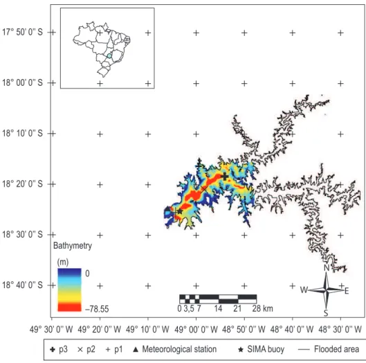
The Itumbiara hydroelectric reservoir (18° 25’ S, 49° 06’ W), classified as case 2 water type (Jerlov, 1968; Nascimento et al., 2011), is located in a region stretched between Minas Gerais and Goiás States (Central Brazil) that was originally covered by tropical grassland savanna. The damming of the Parnaiba River flooded its main tributaries: the Araguari and Corumbá rivers. The basin’s geomorphology resulted in a lake with a dendritic pattern covering an area of approximately 814 km2
and a volume of 17.03 billion m3 (Figure 1).
The climate in the region is characterized by an average precipitation ranging from 2.0 mm in the dry season (May - September) to 315 mm in the rainy season (October - April). In the rainy season the average wind intensity ranges from 1.6 to 2.0 m/s and reaches up to 3.0 m/s in the dry season; the preferential wind direction is southeast. The air temperature in the rainy season (October - April) study of surface water temperatures in hydroelectric
reservoirs is scarce and, in Brazil, is being attempted for the first time.
Several satellites have been launched with spatial, temporal and radiometric resolutions for the study of surface water temperatures with relative accuracy (Steissberg et al., 2005). However, most of these satellites acquire data twice every 16 days, such as Landsat and ASTER (Advanced Spaceborne Thermal Emission and Reflection Radiometer), at any given location. Also, Landsat does not record data at night (unless by special request). The Moderate Resolution Imaging Spectroradiometer (MODIS) onboard the Terra and Aqua satellites overcome these temporal resolution limitations. MODIS data can typically be acquired daily due to their large scan angle (Justice et al., 1998).
Based on this, the aim of this research is to analyze the trends in water surface temperature and their periodical relationship with the heat flux using thermal remote sensing time series.
ranges from 25 to 26.5 °C, decreasing to 21 °C by the beginning of the dry season (June). The relative humidity has a pattern similar to that of the air temperature, but with a small shift in the minimum value towards September (47%). Moreover, during the rainy season the humidity can reach 80% (Alcântara et al., 2010a).
2. Methodological Approach
2.1. Hydrometeorological data
Four hydrometeorological variables were measured from 2003 to 2008 period: the daily mean air temperature (°C), relative humidity (%), wind intensity (m/s) and precipitation (mm). These data were obtained from a meteorological station (see Figure 1 for location) near the dam. The daily mean of each variable was converted into monthly means to adequate it to the time scale of the satellite data.
2.2. Satellite data
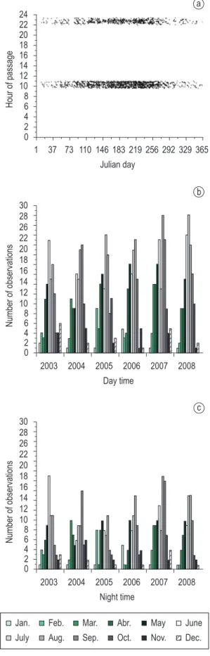
MODIS water surface temperature (WST) level 2, 1 km nominal resolution data (MOD11L2, version 5) were obtained from the National Aeronautics and Space Administration Land Processes Distributed Active Archive Center (Wan, 2008). All available clear-sky MODIS Terra imagery between 2003 and 2008 were selected by visual inspection, resulting in a total of 786 daytime images and 473 nighttime images (Figure 2).
The WST-MODIS data were extensively validated for inland waters and were considered accurate (Oesch et al., 2005,2008; Reinart and Reinhold, 2008; Crosman and Horel, 2009). A shoreline mask to isolate land from water was built using the TM/Landsat-5 image in order to isolate some anomalously cold or warm pixels remaining at some locations near the shoreline of the reservoir (Sentlinger et al., 2008).
The mask was built based on the water level fluctuations in the reservoir; that is, if the MODIS data is from January, then a TM/Landsat-5 was processed take into account the lake level. Each masked MODIS image was checked to assure that each pixel in the border is removed. The mask was built using the NDWI (Normalized Difference Water Index) algorithm proposed by McFeeters (1996) as (Equation 1):
−
= Green NIR+
NDWI
Green NIR (1)
where NIR is the near infrared spectral band.
Figure 2. Information about the MODIS thermal infra-red images: (a) hour of passage and number of satellite imagery available for daytime (b) and nighttime (c).
a
b
where φsf is the sensible heat flux (Wm–2), ra = 1.2 kgm–3 is the air density, c
p = 1.005×10
3 Jkg–1K–1
is the specific heat capacity of air, cH = 1.1×10⁻³ is the
coefficient of turbulent exchange and V = surface wind speed (m/s).
The latent heat flux was computed as follows (Large et al., 1997) (Equation 7):
→
φ = rlf a Ec L V [esat s(T ) re− sat a(T )]0.622
pa (7)
where φlf is the latent heat flux (Wm–2),
cE = 1.1×10⁻³ is a coefficient of turbulent exchange, L = 2.501×10⁶ Jkg–1 is the vaporization of latent heat
and pa is the atmospheric surface pressure (mb). The energy exchange also occurs through precipitation, chemical and biological reactions in the water body, and conversion of kinetic to thermal energy. These energy terms are small enough that should be omitted. Many researchers agree that omitting energy budget components with small values does not significantly affect the results (Bolsenga, 1975; Sturrock et al., 1992; Winter et al., 2003). The sensible and latent heat flux was calculated for daytime and nighttime using the monthly mean surface water temperature derived from MODIS data.
Due to the complexity of these fluxes and the limitations of the atmospheric data available for the area of study, some constraints were imposed. The air temperature (Ta) and wind intensity (V )
were considered the same for the whole reservoir because only one meteorological station was available. Also, the incident solar radiation (φs) was calculated through Equation 2 while considering that the calculated incoming shortwave radiation was the same for the whole reservoir. All heat flux components were computed previously and can be accessed in detail in Alcântara et al. (2010a). 2.4. Correlation between the WST and the heat fluxes
Correlation and multiple regression analyses were carried out to better understand the relationship between the surface water temperature (daytime and nighttime) variability and heat flux terms.
2.5. Time series
We used a 3x3 moving window to smooth original maps and estimate mean values, minimizing noises on output maps and to generate time series in three different reservoir regions: (1) dam, p1, (2) central area, p2, and (3) confluence of the main rivers, p3 (See Figure 1 for location).
2.3. Surface energy budget
The surface energy budget for the Itumbiara reservoir was estimated using lake surface temperature data from the MODIS-WST and surface air temperature, wind speed, and relative humidity data from the hydro-meteorological surface meteorological station.
The exchange of heat across the water surface was computed using the methodology described by Henderson-Sellers (1986) as (Equation 2):
φ = φN s(1 A) (− − φ + φ + φri sf lf) (2)
where φN is the surface heat flux balance, φs is the incident short-wave radiation, A is the albedo of water (=0.07, MacIntyre et al., 2002; Laird and Kristovich, 2002), φri is the Longwave flux, φsf is the sensible heat flux and φlf is the latent heat flux. The units used for the terms in Equation 2 are Wm–2.
The incident short-wave radiation φs was calculated using the following Equation 3:
φ = φa (sin d) (1 0.65C )b1 − 2
s 1 0 (3)
where a1 = 0.79 and b1 = 1.15 are two calibration parameters determined by a comparison with the radiometer data, φ0 = 1390 Wm–2 is the solar
constant, d is the hour angle and C is the cloud cover index, which was estimated using the Reed (1977) empirical relation.
The net longwave radiation corresponding to the outgoing flux minus the incoming flux (LW ↑↓ = LW ↑ – LW ↓), φri is computed as given by Fung et al. (1984) (Equation 4):
φ = εσ − − λ + εσ −
1
4 2 3
T (0.39 0.05e )(1 C) 4 T (T T )
ri s a s s a (4)
where ε = 0.97 is the thermal infrared emissivity of the water, σ is the Stefan-Boltzmann constant, Ts = water surface temperature (K), Ta = surface air temperature (K), λ = 0.8 is the Reed (1977) correction factor, and ea = partial pressure of vapor (mb), which was calculated as (Equation 5):
=
ea resat a(T ) (5)
where r is the relative humidity and esat is the saturation vapor pressure. This was calculated using the polynomial approximation of Lowe (1977).
The non-radiative energy term φrad accounts for the sensible heat flux and latent heat flux. The sensible heat flux was estimated as (Large et al., 1997) (Equation 6):
→
2.6.2. Wavelet analysis
The time frequency space of WST time series was analyzed using the wavelet transform. Wavelet analysis is becoming a common method for analyzing localized variations of power within an environmental time series (Meyers et al., 1993; Kumar and Foufoula-Georgiou, 1997; Massei et al., 2006). Decomposing an environmental time series into time-frequency space allows for the determination of the dominant modes of variability and their modes of variation in time.
Continuous wavelet analysis was applied to WST time series from satellite data using the Morlet wavelet as reference function (the so-called “mother wavelet”). The Morlet wavelet is the most common wavelet transform and consists of a Gaussian-windowed complex sinusoid defined in the time and frequency domains by (Equation 13):
η − ω η − ψ η = π
2
0
1 i
4 2
( ) e e
0 (13)
Where ω0 is the non-dimensional frequency, here assumed to be 6 to satisfy the admissibility condition (Farge, 1992); η is a non-dimensional time parameter and ψ0 (η) is the wavelet function.
Wavelet spectral power at different scale (ω) and time location (τ) can be calculated by (Equation 14):
ω τ = ω τ 2
P ( , )w W( , , x(t) (14)
Where W is the wavelet transform described below.
The continuous wavelet transform of a discrete sequence xn is defined as the convolution of xn with a scaled and translated version of ψ0 (η) (Torrence and Compo, 1998). The wavelet transform W for a given time series x is calculated by (Equation 15):
δ δ
ω = ψ ∗ −
ω ∑= ω
N
t t
x
W ( )n xn (k n)
k ' 1 (15)
Where *indicates the complex conjugate; δt is the uniform time step, k’ is an integer from 1 to N (number of data points) and xn is the time series data. The scale-averaged spectral-power-based wavelet analysis reflects the average variance for different time scales (frequency or period). The calculation procedures of continuous wavelet analysis were coded in Matlab 6.5 (The MathWorks, Inc., Natick, MA).
2.6.3. Cross wavelet, coherence and phase
To show the relationship between WST and the time series identified as statistical significant by the 2.6. Time series analysis
2.6.1. Fourier power spectrum
The WST time series was analyzed using the Fourier power spectrum. The function that implements the transform is given by (Equation 8):
−
+ = +
=
∑
N 1 kn
X(k 1) x(n 1)WN
N 0 (8)
where π − = 2 j N
Wn e , N is the number of points and X is the discrete Fast Fourier Transform of the WST time series.
Data windowing was carried out to avoid leakage in the estimation of the periodogram. Data windowing modifies the relationship between the spectral estimate at discrete frequencies and its continuous (periodogram) spectrum at nearby frequencies. There are many window functions used to prevent spectral leakage, most of them rising from zero to a peak and then falling again. This paper uses Hanning and Hamming windows (Press et al., 1992). The first was used to prevent leakage while the last was used to smooth the resulting spectra. The Hanning and Hamming window coefficients are show in (Equation 9 and 10), respectively:
= − π − =
n
w(n) 0.5 1 cos 2 ,n 1...N
N 1 (9)
= − π =
−
n
w(n) 0.54 0.46 cos 2 ,n 1...N
N 1 (10)
Power spectrum smoothing reduces the variance and increases the statistical confidence, or reduces the confidence limits. In the algorithm implementation there must be a compromise between strong (more confidence but stronger bias) and weak smoothing (less confidence but less bias). In this work smoothing was carried out with a variable length Hamming window. The inferior and superior confidence limits for the spectra area, respectively, are given by (Equation 11 and 12):
=
χ df CLinf a df , 2 (11) = − χ
df
CLinf 1 a
df ,
2 (12)
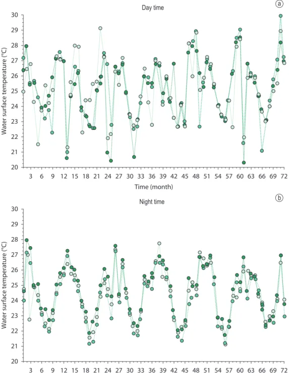
Also is easy to observe in all time series (daytime and nighttime) a cyclical pattern, passing for a minimum (June - July) and a maximum (December and January). This cyclical pattern can be analyzed through the Fourier and the Wavelet Analysis. 3.2. Fourier power spectrum
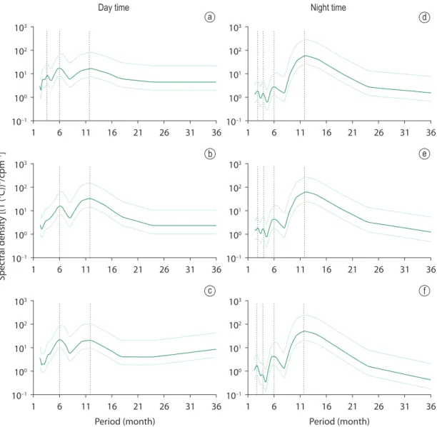
The Figure 4 shows the Fourier Power Spectrum for both daytime or nighttime WST. The daytime time series, p1 (Figure 4a) and p2 (Figure 4b) presents two peaks with same periods, that is the annual cycle and the semiannual cycle. The period of 4.5 months appear only in the p1 time series. The maximum density for the time series p1 and p2 occurs for periods of 6 and 12 months, respectively. The time series p3 (Figure 4c) shows a high density for periods of 6 months, followed by 12 and 36 months.
The analysis of nighttime WST for p1 (Figure 4d), p2 (Figure 4e) and p3 (Figure 4f ) shows that the highest spectral density were 12, 6, 3 and 2 months. As was emphasized by Kaiser (1994) the Fourier transform can hidden periods with significant spectral density, by imposing a scale or response interval dependent of the time series size (in our case 72 months). Based on this Kaiser suggested a time-frequency analysis using the Wavelet Power Spectrum.
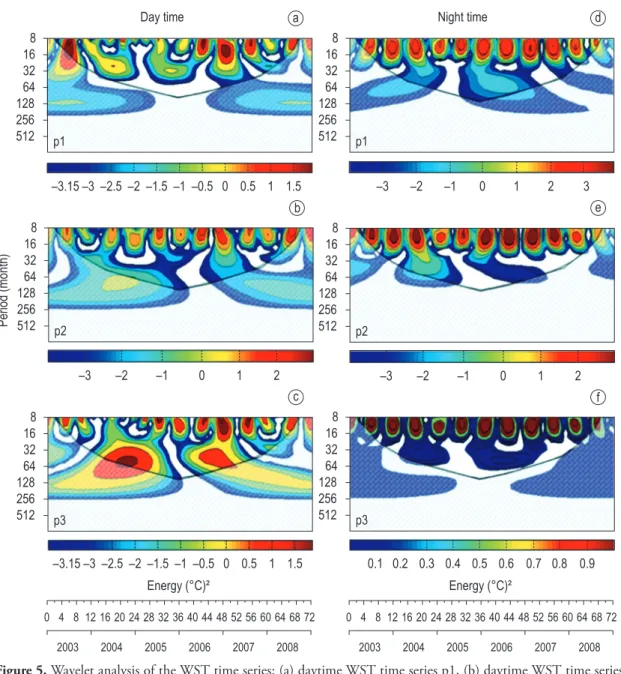
3.3. Wavelet analysis
The time series obtained from the MODIS/Terra images shows that the principal range of variability is from 8 to 24 months. The time series p1 (Figure 5a) shows that for the year 2003 (from June to July) the maximum peak of energy occurs for periods ranging from 8 to 12 months. From year 2004 (months of May, September and December) to 2005 (March and April) the higher energy peak occurs for periods bellow 8 months (probably 6 months, as showed by the Fourier power spectrum).
In 2006 the energy peaks occurs in May, June, November and December with periods until 24 months; whereas in 2007 the peaks occurs in May, June and July with periods of significantly variability up to 12 months. In 2008 only a small peak of energy, if compared with others years, was observed during May for periods smaller than 12 months.
The time series p2 (Figure 5b) shows that highest energy peaks not exceed periods of 12 months in all years of analysis. The months which showed these highest or maximum spectral density were the same Pearson’s correlation coefficient, the cross wavelet
analysis was carried out and the coherence and phase analyzed (Grinsted et al, 2004).
The cross wavelet transform of two time series xn and yn is defined as Wxy = WxWy*, where *denotes
complex conjugation, so the cross wavelet power could be defined as |Wxy| (Grinsted et al. 2004). The interpretation of complex argument arg (W) can be interpreted as the local relative phase between xn and yn in time frequency space. The cross wavelet power theoretical distribution of two time series with background power spectra Px
k and P y
k is given in Torrence and Compo (1998) as (Equation 16):
< = σ σ y* x
W (s)W (s)n n Z (p) y x v
D p P Pk k
v
x y (16)
where Zv (p) is the confidence level associated with the probability p for a probability density function (pdf) defined by the square root of the product of two χ2 distributions. Cross wavelet power reveals
areas with high common power.
Another useful measure is how coherent the cross wavelet is in time frequency space. The wavelet coherence could be defined following Torrence and Webster (1999) as (Equation 17):
− = − − 2 wy 1 S(s Wn (s)) 2
R (s)n 2
2 y
1 x 1
S(s W (s) ).S(sn W (s) )n
(17)
where S is a smoothing operator; Notice that this definition closely resembles that of a traditional correlation coefficient, and is useful to think of the wavelet coherence as a localized correlation coefficient in time frequency space. The calculation procedures of cross wavelet and wavelet coherence were coded in Matlab 6.5 (The MathWorks, Inc., Natick, MA).
3. Results and Discussion
3.1. Water surface temperature (WST) time series The time series of WST measured by satellite are show in Figure 3. The WST measured during daytime and nighttime in Figure 3a,b, respectively.
a
b
Figure 3. Time series (3x3) of monthly mean water surface temperature (WST) in three selected stations (p1, p2 and p3) from 2003 to 2008: (a) daytime WST, (b) nighttime WST. Where p1 was taken near the dam, p2 in central region and p3 in the river confluence (see Figure 3 for location).
that was previously presented for the time series p1 (Figure 5a).
For the time series p3 (Figure 5c) there is energy peaks up to 60 months (five years) occurring in 2004 for months of September and December. Also as was verified before in time series p1 and p2, energy
peaks of 24 months occur in December 2006. We also found peaks for periods of 60 months in May 2006 and February 2007.
3.4. Statistical model for daytime and nighttime water surface temperatures
The Pearson correlation computed between the daytime and nighttime WST derived from the MODIS image against the heat flux terms is shown in Table 1. For daytime temperatures, the only significant variable correlated heat flux was the shortwave radiation; for nighttime temperatures, it was the longwave radiation, latent heat flux and sensible heat flux.
The multiple regression analysis shows that for daytime WST, the correlated heat flux terms explain 89% of its annual variation (RMS = 0.89 °C, p < 0.0013). For nighttime, the heat flux terms explain 94% (RMS = 0.53 °C, p < 0.0002). The representative Equations of these relationships are presented in Equations 18 and 19:
best defined and with smaller energy than those of daytime time series. Also it is a fact that, in general way, the months with maximum density energy includes the periods from May to August and from November to April of the subsequent year. In these cases a little delay were recorded in some samples.
The time series of nighttime WST of highest energy was the p1 (Figure 5d) followed by the time series p2 (Figure 5e) and with a smallest spectral density the p3 (Figure 5f). In the case of p3 the highest energy was observed for small periods, less than 16 months and small energy for periods higher than 20 months.
An analysis of correlation between the WST and the heat flux components was computed to check out the relative importance of each heat flux in the WST time series.
d a
f b
c
e
when the shortwave radiation increases, the air temperature increases and transfers heat in the water column. However, the pattern of wind intensity and direction during the day is also important; with high wind intensity, the surface water loses heat through convection.
At night, the processes of convection and advection acting at the surface water and the balance of longwave radiation are important to drive the water temperature. Because of this, Equation 18 is a subtraction of the joint effects of these three important fluxes.
= + φ
Tdaytime 18.78 (0.02 )S (18)
= − φ + + φ
Tnighttime 38.17 (0.31 ri) (0.55 ) (0.39lf sf) (19)
where Tdaytime is the daytime water surface temperature (°C), Tdaytime is the nighttime water surface temperature (°C), φS is the short wave radiation (Wm–2), φ
ri is the long wave radiation (Wm–2), φ
lf is the latent flux (Wm
–2) and φ Sf is the sensible flux (Wm–2).
Only the incoming shortwave radiation was needed to model the daytime WST. This is because
Figure 5. Wavelet analysis of the WST time series: (a) daytime WST time series p1, (b) daytime WST time series p2, (c) daytime WST time series p3, (d) nighttime WST time series p1, (e) nighttime WST time series p2 and (f) nighttime WST time series p3. Cross-hatched regions on either end indicate the “cone of influence,” where edge effects become important.
f e d a
b
January and July 2007, with φri advanced 90° [~27 days]; (3, 4) band period of 5-6 months end of 2005 until the beginning of 2006, with φri
advanced 135° [~2 months]; and (5) band period of 9-15 months localized between January 2004 until November 2007, with φri advanced 135° [~6 months].
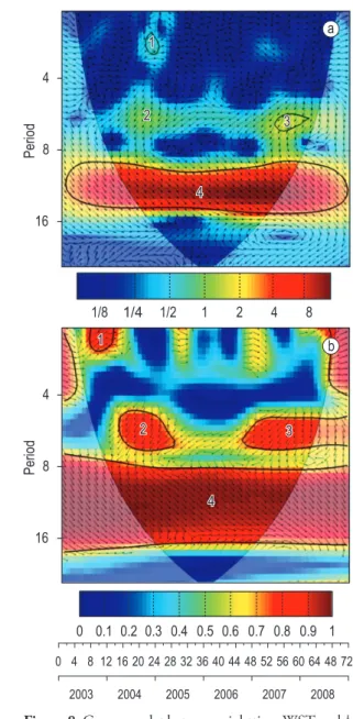
3.5.3. Nighttime water surface temperature versus sensible flux (φsf)
The cross wavelet analysis between the nighttime WST and φsf is show in the Figure 8. Four high common power were identified, (1) band period of 2-3 months localized from September to December 2004 (Figure 8a), with φsf retarded 45° [~9 days] in 3.5. Cross wavelet, coherence and phase
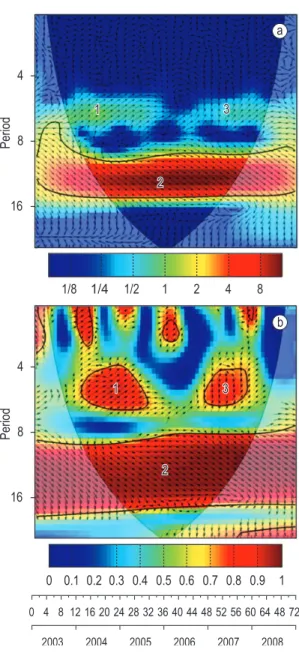
3.5.1. Daytime water surface temperature versus shortwave radiation (φS)
The cross wavelet between the daytime WST and the φS shows two band period of high common power, the first in the band period of 4.5-7 (regions 1 and 3) months, in special from years of 2004 and 2007; the second with the highest common power between 9-15 months (region 2) also with special attention in the years of 2004 and 2007 (Figure 6a). The coherence in those common power periods (Figure 6b) shows that for the region 1 (period of 4-7 months) the φS is retarded 45° [~21 days] in relation to WST (from January 2004 to July 2005). That is, for a period from 4-7 months when the φS
presents a peak of variability the WST needs 21 days to present like a response to this solar enhancement. The El-Niño was present during 2004-2005 years and can affect the regional climate, principally the air moisture and the rainfall regime.
For the region 2 (period of 8-16.5 months) the
φS is advanced 45° [~1.5 months] in relation to WST. In this case, for periods higher than 8 months the WST tends to reach their maximum variability but the φS will present its higher variability 1.5 months later. The region 3 (band period of 4.5-6.5) is representative of the 2007 year (La-Niña year) with the φS is retarded 90° [~1.25 months] in relation to WST.
3.5.2. Nighttime water surface temperature versus longwave radiation (φri)
The cross wavelet analysis between the nighttime WST and φri is show in the Figure 7. Five high common power was identified: (1) band period of 1-2 months localized between November 2004 and April 2005 (Figure 7a), with φri advanced 45° [~6 days] in relation to nighttime WST (Figure 7b); (2) band period of 3-4 months localized between Table 1. Pearson correlation coefficients for daytime and nighttime surface temperatures against shortwave radia-tion (φs), longwave radiation (φri), sensible flux (φsf), and latent flux (φlf).
Daytime water temperature
Nighttime water temperature
φs 0.64 (p = 0.03) –
φri 0.06 (p = 0.46) –0.65 (p = 0.00)
φsf 0.39 (p = 0.08) 0.42 (p = 0.00)
φlf 0.60 (p = 0.26) –0.64 (p = 0.00)
Figure 6. Cross wavelet between daytime WST and φS (a) and the coherence and phase (b).
a
to April 2005 (Figure 9a), with φlf retarded 45° [~8 days] in relation to nighttime WST (Figure 9b); (2, 3) band period of 6-8 months localized from April 2004 to January 2005, with φlf retarded 90° [~1.7 months]; (4) band period of 9-15 months between February 2004 to November 2007, with
φlf and nighttime WST in anti-phase.
The WST variability is not only due to heat flux (shortwave, longwave, sensible and latent), but also the physical processes that occur into the water column (Alcântara et al., 2011b). According to Alcântara et al. (2010b) the passage of cold front over the reservoir can modify the heat flux and consequently the WST. The cold front enhances the convective processes in the water column, relation to nighttime WST (Figure 8b); (2) band
period of 5-7 months localized from April 2004 to April 2005, with φsf advanced 135° [~2 months]; (3) band period of 5.5-7 months between May 2007 to March 2008, with φsf advanced 135° [~2 months]; and (4) band period of 9-15 months localized between February 2004 until November 2007, with φri advanced 45° [~2 months].
3.5.4. Nighttime water surface temperature versus latent flux (φlf)
The cross wavelet analysis between the nighttime WST and φlf is show in the Figure 9 and were identified four high common power, (1) band period of 1-3 months localized from August 2004
a
b
Figure 8. Cross wavelet between nighttime WST and φsf (a) and the coherence and phase (b).
a
b
presents a good agreement for periods of 6 (with shortwave retarded) and 12 months (with shortwave advanced);
• For nighttime WST and longwave the good agreement is present for 1, 3, 6 and 12 months, all with longwave advanced in relation to WST;
• The nighttime WST and sensible flux high common power for band periods of 2 (re-tarded), 6 (advanced) and 12 (advanced); • Finally, the nighttime WST and latent flux
with band periods of 2 (retarded), 6 (retarded) and 12 months (WST and latent flux in anti-phase).
Acknowledgements
The authors would like to thank the FAPESP Project 2007/08103-2, INCT for Climate Change project (grant 573797/2008-0 CNPq). Enner Alcântara thanks CAPES grant 0258059.
References
ALCÂNTARA, E., STECH, J., LORENZZETTI, J., BONNET, M., CASAMITJANA, X., ASSIREU, A. and NOVO, E. 2010a. Remote sensing of water surface temperature and heat flux over a tropical hydroelectric reservoir. Remote Sensing of Environment, vol. 114, p. 2651-2665. http://dx.doi. org/10.1016/j.rse.2010.06.002
ALCÂNTARA, E., BONNET, M-P., ASSIREU, AT., STECH, JL., NOVO, EMLM. and LORENZZETTI, JA. 2010b. On the water thermal response to the passage of cold fronts: initial results for Itumbiara reservoir (Brazil). Hydrology and Earth System Sciences Discussions, vol. 7, p. 9437-9465. http://dx.doi. org/10.5194/hessd-7-9437-2010
ALCÂNTARA, E., NOVO, EM., BARBOSA, CF., BONNET, M-P., STECH, J. and OMETTO, JP. 2011a. Environmental factors associated with long-term changes in chlorophyll-a concentration in the Amazon floodplain. Biogeosciences Discussion, vol. 8, p. 3739-3770. http://dx.doi.org/10.5194/ bgd-8-3739-2011
A LC Â N TA R A , E . a n d S T E C H , J . 2 0 1 1 b. Desenvolvimento de modelo conceitual termodinâmico para o reservatório hidrelétrico de Itumbiara baseado em dados de satélite e telemétricos. Revista Ambiente & Água, vol. 6, p. 157-179. BOLSENGA, S. 1975. Estimating energy budget
components to determine Lake Huron evaporation. Water Resources Research, vol. 11, p. 661-666. http://dx.doi.org/10.1029/WR011i005p00661 BONNET, MP., POULIN, M. and DEVAUX, J. 2000.
Numerical modeling of thermal stratification in a lake reservoir: Methodology and case study. modifying the vertical temperature profile and
consequently the temperature distribution in the water surface.
4. Conclusions
The results obtained allow reaching the following conclusions:
• If we assume that the water surface tem-perature (WST) could be explained only the heat fluxes then for daytime WST only the shortwave radiation explain 89% of the temperature variability; to nighttime WST the longwave, sensible and latent flux explain 94%;
• The daytime WST and shortwave radiation Figure 9. Cross wavelet between nighttime WST and φlf (a) and the coherence and phase (b).
a
LARGE, WG., DANABASOGLU, G. and DONEY, SC. 1997. Sensitivity to surface forcing and boundary layer mixing in a global ocean model: Annual-mean climatology. Journal of Physical Oceanography, vol. 27, p. 2418-2447. http://dx.doi.org/10.1175/1520-0485(1997)027%3C2418:STSFAB%3E2.0.CO;2 LERMAN, A., IMBODEN, D. and GAT, J. 1995.
Physics and chemistry of lakes. Berlin: Springer-Verlag. http://dx.doi.org/10.1007/978-3-642-85132-2 LOWE, PR. 1977. An approximating polynomial for the
computation of saturation vapor pressure. Journal of Applied Meteorology, vol. 16, p. 100-103. http:// dx.doi.org/10.1175/1520-0450(1977)016%3C010 0:AAPFTC%3E2.0.CO;2
MASSEI, N., DUPONT, JP., MAHLER, BJ., LAIGNEL, B., FOURNIER, M., VALDES, D. and OGIER, S. 2006. Investigating transport properties and turbidity dynamics of a karst aquifer using correlation, spectral, and wavelet analyses. Journal of Hydrology, vol. 329, p. 244-257. http://dx.doi.org/10.1016/j. jhydrol.2006.02.021
MACINTYRE, S., ROMERO, JR. and KLING, GW. 2002. Spatial variability in surface layer deepening and lateral advection in an embayment of Lake Victoria, East Africa. Limnology and Oceanography, vol. 47, p. 656-671. http://dx.doi. org/10.4319/lo.2002.47.3.0656
MCFEETERS, SK. 1996. The use of the Normalized Difference Water Index (NDWI) in the delineation of open water features. International Journal of Remote Sensing, vol. 17, p. 1425-1432. http://dx.doi. org/10.1080/01431169608948714
MEYERS, SD., KELLY, BG. and O’BRIEN, JJ. 1993. An introduction to wavelet analysis in Oceanography and Meteorology: with application to the dispersion of Yanai Waves. Monthly Weather Review, vol. 121, p. 2858-2866. http://dx.doi.org/10.1175/1520-0493(1993)121%3C2858:AITWAI%3E2.0.CO;2 MORENO-OSTOS, E., MARCÉ, R., ORDÓÑEZ, J.,
DOLZ, J. and ARMENGOL, J. 2008. Hydraulic management drives heat budgets and temperature trends in a Mediterranean reservoir. International Review of Hydrobiology, vol. 93, p. 131-147. http://dx.doi.org/10.1002/iroh.200710965
NASCIMENTO, RFF., ALCÂNTARA, E., KAMPEL, M. and STECH, JL. 2011. Caracterização limnológica do reservatório hidrelétrico de Itumbiara, Goiás, Brasil. Revista Ambiente & Água, vol. 6, p. 143-156. O E S C H , D . , J A Q U E T, J - M . , H A U S E R ,
A. and WUNDERLE, S. 2005. Lake surface water temperature using advanced very high resolution radiometer and moderate resolution imaging spectroradiometer data: validation and feasibility study. Journal of Geophysical Research, vol. 10(C12014), p. 1-17.
Aquatic Science, vol. 62, p. 105-124. http://dx.doi. org/10.1007/s000270050001
CHAPRA, SC. 1997. Surface Water-Quality Modeling. New York: McGraw-Hill.
CROSMAN, ET. and HOREL, JD. 2009. MODIS-derived surface temperature of the Great Salt Lake. Remote Sensing of Environment, vol. 113, p. 73-81. http://dx.doi.org/10.1016/j.rse.2008.08.013 FARGE, M. 1992. Wavelet transforms and their
applications to turbulence. AnnualReview ofFluid Mechanics, vol. 24, p. 395-457.
FUNG, IY., HARRISON, DE. and LACIS, AA. 1984. On the variability of the net longwave radiation at the ocean surface. Reviews of Geophysics, vol. 22, p. 177-193. http://dx.doi.org/10.1029/RG022i002p00177 GRINSTED, A., MOORE, JC. and JEVREJEVA,
S. 2004. Application of the cross wavelet transform and wavelet coherence to geophysical time series. Nonlinear Processes in Geophysics, vol. 11, p. 561-566. http://dx.doi.org/10.5194/npg-11-561-2004 HENDERSON-SELLERS, B. 1986. Calculating the
Surface Energy Balance for Lake and Reservoir Modeling: A Review. Reviews of Geophysics, vol. 24, p. 625-649. http://dx.doi.org/10.1029/ RG024i003p00625
JERLOV, NG. 1968. Optical Oceanography. New York: Elsevier.
JUSTICE, CO., VERMOTE, E., TOWNSHED, JRG., DEFRIES, R., ROY, DP., HALL, DK., SALOMONSON, VV., PRIVETTE, JL., RIGGS, G., STRAHLER, A., LUCHT, W., MYNENI, RB., KNYAZIKHIN, Y., RUNNING, SW., NEMANI, RR., WAN, Z., HUETE, AR., VAN-LEEUWEN, W., WOLFE, RE., GIGLIO, L., MULLER, JP., LEWIS, P. and BARNSLEY, MJ. 1998. The moderate Resolution Imaging Spectroradiometer (MODIS): land remote sensing for global change research. IEEE Transactions on Geoscience and Remote Sensing, vol. 36, p. 1228-1247. http://dx.doi.org/10.1109/36.701075 KAISER, G. 1994. A friendly guide to wavelets.
Birkhäuser. 300 p.
KIMMEL, BL., LIND, OT. and PAULSON, LJ. 1990. Reservoir primary production. In THORTON, KW., KIMMEL, BL., PAYNE, FE., eds. Reservoir limnology. Ecological Perspectives. New York: John Wiley and Sons.
KUMAR, P. and FOUFOULA-GEORGIOU, E. 1997. Wavelet analysis for geophysical application. Reviews of Geophysics, vol. 35, p. 385-412. http://dx.doi. org/10.1029/97RG00427
STEISSBERG, TE., HOOK, SJ. and SCHLADOW, SG. 2005. Characterizing partial upwellings and surface circulation at Lake Tahoe, California-Nevada, USA with thermal infrared images. Remote Sensing of Environment, vol. 99, p. 2-15. http://dx.doi. org/10.1016/j.rse.2005.06.011
STURROCK, A., WINTER, T. and ROSENBERRY, D. 1992. Energy budget evaporation from Williams Lake: a closed lake in north central Minnesota. Water Resources Research, vol. 28, p. 1605-1617. http://dx.doi.org/10.1029/92WR00553
THIEMANN, S. and SCHILLER, H. 2003. Determination of the bulk temperature from NOAA/AVHRR satellite data in a midlatitude lake. International Journal of Applied Earth Observation and Geoinformation, vol. 4, p. 339-349. http://dx.doi. org/10.1016/S0303-2434(03)00021-7
TORRENCE, C. and COMPO, GP. 1998. A Practical Guide to Wavelet Analysis. Bulletin of the American Meteorological Society, vol. 79, p. 61-78. http://dx.doi. org/10.1175/1520-0477(1998)079%3C0061:APG TWA%3E2.0.CO;2
TORRENCE, C. and WEBSTER, P. 1999. Interdecadal changes in the ENSO-Monsoon system. Journal of Climate, vol. 12, p. 2679-2690. http://dx.doi. org/10.1175/1520-0442(1999)012%3C2679:ICI TEM%3E2.0.CO;2
WAN, Z. 2008. New refinements and validation of the MODIS land-surface temperature/emissivity products. Remote Sensing of Environment, vol. 112, p. 59-74. http://dx.doi.org/10.1016/j. rse.2006.06.026
WINTER, T., BUSO, D., ROSENBERRY, D., LIKENS, G., STURROCK, JA. and MAU, D. 2003. Evaporation determined by the energy-budget method for Mirror Lake, New Hampshire. Limnology and Oceanography, vol. 48, p. 995-1009. http://dx.doi.org/10.4319/lo.2003.48.3.0995
Received: 07 June 2011 Accepted: 14 December 2011 OESCH, D., JAQUET, J-M., KLAUS, R. and
SCHENKER, P. 2008. Multi-scale thermal pattern monitoring of a large lake (Lake Geneva) using a multi-sensor approach. International Journal of Remote Sensing, vol. 29, p. 5785-5808. http://dx.doi. org/10.1080/01431160802132786
PRESS, WH., TEUKOLSKY, SA., VETTERLING, WT. and FLANNERY, BP. 1992. Numerical recipes in fortran 77: the art of scientific computing. Cambridge University Press. 933 p. vol. 1 of Fortran numerical recipes.
REED, R. 1977. On estimating insolation over the ocean. Journal of Physical Oceanography, vol. 7, p. 482-485. http://dx.doi.org/10.1175/1520-0485(1977)007%3C0482:OEIOTO%3E2.0.CO;2 REINART, A. and REINHOLD, M. 2008. Mapping
surface temperature in large lakes with MODIS data. Remote Sensing of Environment, vol. 112, p. 603-611. http://dx.doi.org/10.1016/j.rse.2007.05.015 S C H L A D OW, S G . , PA L M A R S S O N , S O . ,
STEISSBERG, TE., HOOK, SJ. and PRATA, FJ. 2004. An extraordinary upwelling event in a deep thermally stratified lake. Geophysical Research Letters, vol. 31, p. L15504. http://dx.doi. org/10.1029/2004GL020392
SENTLINGER, GI., HOOK, SJ. and LAVAL, B. 2008. Sub-pixel water temperature estimation from thermal-infrared imagery using vectorized lake features. Remote Sensing of Environment, vol. 112, p. 1678-1688. http://dx.doi.org/10.1016/j. rse.2007.08.019