Validation of Additive Manufacturing Process Trough Build Simulation

Herberto Gastão de Martins e Beaumont

Validation of Additive Manufacturing

Process Trough Build Simulation

Dissertation submitted in partial fulfilment of the requirements for the degree of

Master of Science in

Industrial Engineering and Management

Supervisor: Ana Sofia Leonardo Vilela de Matos,

PhD, Faculdade de Ciências e Tecnologia,

Universidade Nova de Lisboa

Júri:

Presidente: PhD Maria Celeste Rodrigues Jacinto Vogais: PhD Helena Maria Carvalho Remígio PhD Ana Sofia Leonardo Vilela de Matos

Validation of additive manufacturing process through build simulation Copyright © 2018 Herberto Gastão de Martins e Beaumont Faculdade de Ciências e Tecnologia e Universidade Nova de Lisboa A Faculdade de Ciências e Tecnologia e a Universidade Nova de Lisboa têm o direito, perpétuo e sem limites geográficos de arquivar e publicar esta dissertação através de exemplares impressos reproduzidos em papel ou de forma digital, ou por qualquer outro meio conhecido ou que venha a ser inventado, e de a divulgar através de repositórios científicos e de admitir a sua cópia e distribuição com objetivos educacionais ou de investigação, não comerciais, desde que seja dado crédito ao autor e editor.

For M. & S. In any given order… or mixed together

Acknowledgements

The writing of this document led naturally to research on other colleagues works. From those readings I came to realise the importance of acknowledgements. It is hard to define the beginning of external influence in the making of this text and I’m most likely to be inaccurate and leave some of the contributors out of this paragraph. Furthermore, from reading other dissertations I frequently got the feeling that the acknowledgments section usually went above the work itself and embraced simultaneously the recognition for the end of a cycle.

Hence, without skipping tradition but bearing in mind that the only achievement is more responsibility and not the end, but the beginning of something new, I would like to acknowledge, the help, contribution, criticism and challenges provided by the following:

From my school, professor Rogério Puga Leal for allowing me to start an unexpected adventure. It’s never easy to go against one’s intuition. Professor Ana Sofia Matos, for the endless confidence that I always felt emanating from her, a crucial factor given the physical distance.

From my workplace, everyone without exception for creating a great environment of continuous learning and application, making every day fun and enjoyable. For the support in the making of this work to Desi Bacheva, Keith Parker, Evert Hooijkamp, Sarah Jenkins, Lucia Revilla, Henry Greenhalgh. For the help, support, and specially freedom that they gave me in all the decisions of this work process.

Resumo

A produção de componentes através de processos de produção aditiva (PA) permite uma enorme liberdade na criação de peças com formas complexas cujo fabrico seria impossível através de métodos convencionais. Esta liberdade no entanto, tem os seus limites. Por essa razão quando se projeta para PA é necessário ter em conta as seguintes características, não exclusivas: espessuras variáveis, canais internos, elementos suspensos, suportes (posição e remoção), redes, e, ao mesmo tempo, evitar a distorção do componente. Entretanto a física que opera estas mudanças é de difícil prevenção particularmente à micro-escala. De modo a controlar ou prever as consequências deste processo produtivo, soluções como simulação dos processos de PA começaram a ser testadas como substituto de testes destrutivos. Finalmente os materiais usados desempenham um papel importante na ligação entre design e tensões térmicas influenciando o comportamento do(s) elemento(s) produzido(s). Neste trabalho um conjunto de dimensões geométricas foi escolhido de modo a validar e conduzir um teste de sensibilidade no programa MS Simufact, para que mais trabalho nesta área possa ser desenvolvido. O conjunto de dimensões escolhidas foram os diâmetros e as circularidades de três anéis concêntricos. Todos os vários inputs foram analisados e explicados. Foram considerados dois materiais durante a simulação, inconel 625 para os componentes (pó metálico da peça) e aço inoxidável para a base onde a peça é construída. Com base nas presunções da teoria e funções do programa, o input central a ser estudado nesta fase inicial foi o tamanho dos voxels. Simultaneamente através de um desenho de experiências, outros parâmetros e o seu peso foram estudados de modo a determinar os valores de input que forneciam o melhor resultado. Os resultados da simulação foram comparados com peças produzidas e medidas por um sistema de medição ótico 3D.

Palavras-chave: Produção aditiva, Selective Laser Melting, Simulação de Tensões Térmicas, Voxel, Inconel 625.

Abstract

Producing parts trough Additive Manufacturing (AM) processes enables tremendous freedom in creating components with free-form and intricate features that would be impossible to manufacture through conventional methods. This freedom however does not come without its limits. Thus, when designing for AM (DfAM) one should consider, amongst which but not exclusively, variable wall thickness, deep channels, overhanging features, supports (position and support removal), lattices, as well as avoiding component distortion. Meanwhile the physics commanding these changes are hard to predict particularly in the micro-scale. To eliminate or minimize such problems solutions like build simulation have started to be looked at as a replacement for unwanted destructive tests. Finally, the materials used play a big role linking design and thermal stresses to feature behaviour. In this work a set of features was chosen to validate and conduct a sensitivity test on MS Simufact simulation software, so that future work in this area can be continued. The set of features chosen, were the diameters and roundness of three concentric rings. All the various inputs were analysed throughout this work and explained. Two materials were considered in the experiment, alloy Inconel 625 for the build powder with a stainless-steel build plate base. From the assumptions taken and software functions the first and main input to be studied was the voxel size. A relation between the simulated feature and the optimal voxel size is what is intended to be achieved. Simultaneously via Design of Experiments (DOE), other parameters were studied to assess their overall effect on result. The Simulation run results were compared with actual measured parts via a 3D optical measuring system.

Keywords: Additive Manufacturing, Selective Laser Melting, Thermal Stresses Simulation, Voxel Finite Elements, Inconel 625;

Table of Contents

List of abbreviations ... xiii

1 Introduction ... 1

1.1 Motivation ... 1

1.2 Objectives ... 2

1.3 Plan, resources and document structure ... 2

1.4 Proposed Methodology ... 3

2 Additive Manufacturing ... 5

2.1 Introduction to Additive Manufacturing ... 5

2.2 Selective Laser Melting Controllable Factors ... 7

2.2.1 Set-Up Parameters ... 8

2.2.2 Fill Hatch ... 10

2.3 Selective Laser Melting Non-Controllable Factors ... 11

2.4 Context of the Experimental Study………13

2.4.1 Renishaw AM 250 ... 13

2.4.2 Inconel 625 ... 14

2.4.3 HiETA Technologies ... 15

2.5 Thermal Stresses ... 15

2.5.1 Basic definitions ... 15

2.5.2 Inherent strains ... 16

2.5.3 Equations of Equilibrium... 17

3 Experimental Setup ... 19

3.1 Ms Simufact Additive AM ... 19

3.2 Marc Solver ... 19

3.3 Voxel ... 20

3.4 Simulation Parameters ... 21

3.4.1 Process ... 22

3.4.2 Component ... 22

3.4.3 Manufacturing ... 23

3.4.4 Analysis ... 24

3.5 Optical Measuring System ... 25

4 Experiment Methods ... 29

4.4 Case Study Model ... 29

4.5 Calibration ... 30

4.3 Build Design ... 33

4.4 Design of Experiments ... 35

4.5 Results and Discussion ... 37

4.5.1 Simulation runs ... 37

4.5.2 Discussion ... 42

4.6 Confirmation Experiments ... 44

4.6.1 Calibration Test ... 45

4.6.2 AM Machine ... 45

5 Conclusions and Future work ... 51

Bibliography ... 53

Index of figures

Figure 2.1 Overview of metal AM process ... 7

Figure 2.2 Selective Laser Melting: (a) SLM process; (b) Platform Cycle ... 8

Figure 2.3 (a) Isometric view (left-hand); (b) Plan view (right-hand) of a melting pool

shape ... 9

Figure 2.4 (a) Diameter of focal point. On Renishaw AM machines the average

diameter of the focal point is 75 µm and the focal point around 2 mm. Giving a ±1 mm

tolerance (left hand side); (b) Focal point in relation to datum line (left hand side) ... 10

Figure 2.5 Hach types; (a) Meander (left hand side); (b) Stripes (middle); (c)

Chessboard (right hand side) ... 11

Figure 2.6 Actual part (a); Simulation run (b); The colour map was set at the same scale

for both parts and the gas pattern was missed by the simulation. The deviation labels

shown are in millimetres ... 12

Figure 2.7 Ren AM250 (a); Ren AM250 Build Chamber (b) ... 14

Figure 2.8 Determination of the equations of equilibrium ... 17

Figure 3.1 Voxel mesh of three layers; source ... 20

Figure 3.2 Control points for one voxel ... 21

Figure 3.3 Simufact Status bar ... 21

Figure 3.4 Build selection menu ... 24

Figure 3.5 Meshing properties ... 25

Figure 3.6 Macro image processing system ... 26

Figure 3.7 Atos gom scanner ... 27

Figure 4.1 Flowchart of the applied model ... 30

Figure 4.2 Calibration samples before and after cutting (a and (b respectively ... 31

Figure 4.3 Calibration results ... 32

Figure 4.4 Ring Build ... 33

Figure 4.5 Summary of the three ring builds ... 34

Figure 4.6 Significant factors on the diameter 1 response... 39

Figure 4.7 Significant factors on the diameter 2 response... 39

Figure 4.8 Significant factors on diameter 3 response ... 39

Figure 4.9 Significant factors on roundness 1 response ... 40

Figure 4.10 Significant factors on roundness 2 response ... 40

Figure 4.11 Significant factors on roundness 3 response ... 40

Figure 4.12 Sensitivity analysis and best combination of factors (not targeting

Roundness) ... 41

Figure 4.13 Actual Build number 1 ... 42

Figure 4.14 Actual Build number 2 ... 43

Figure 4.15 Actual Build number 3 ... 43

Figure 4.16 Simulation optimization result (-0.5 mm to 0.5 mm scale) ... 44

Figure 4.17 Simulation optimization result (-0.05 mm to 0.05 mm scale) ... 44

Figure 4.18 Simulation optimization result with estimated calibration values (-0.5 mm

to 0.5 mm

) ... 45

Figure 4.19 Summary of the three ring builds (2

AM250) ... 46

Figure 4.21 Actual Build 2 (2

AM250) ... 47

Figure 4.22 Actual Build 3 (2

_{AM250) ... 48}

Figure 4.23 Updated flowchart of the model ... 49

Index of tables

Table 2.1 AM Categories ... 5

Table 2.2 Developmental AM Categories ... 6

Table 2.3 Controllable Inputs ... 8

Table 2.4 Fill hatch

10

Table 2.5 Composition of Inconel 625 ... 14

Table 2.6 Inconel 625 properties ... 15

Table 2.7 Thermal Domain of analysis in SLM ... 15

Table 2.8 Fundamental modes of heat transfer ... 16

Table 3.1 FEA linear analysis variables ... 19

Table 3.2

widget parameters ... 22

Table 3.3 Component widget parameters ... 23

Table 3.4 Manufacturing widget parameters ... 23

Table 3.5 Analysis widget parameters ... 24

Table 3.6 Studied variables ... 25

Table 3.7 Basic

of an Optical Measuring System ... 26

Table 4.1

Ø and roundness values for all three rings ... 33

Table 4.2 Targeted values for Optimization ... 34

Table 4.3 Randomized design table of the experiments ... 36

Table 4.4 Simulation results ... 37

Table 4.5

and SD of the simulation runs ... 38

Table 4.6 Run number and replicates relation ... 38

List of abbreviations

3D Three-Dimensional AM Additive Manufacturing ANOVA Analysis of Variance

ASTM American Society for Testing and Materials CAD Computer-aided Design

CAE Computer-aided Engineering CFD Computational Fluid Dynamics

CLIP Continuous Liquid Interface Production CMM Coordinate Measuring System

DED Directed Energy Deposition DfAM Design for AM

DOE Design of experiments EBW Electron Beam Welding FE Finite elements

FEA Finite Element Analysis

GD&T Geometric Dimensioning & Tolerance HAZ Heat Affected Zone

LBW Laser Beam Welding

LOM Laminated Object Manufacturing

NASA National Aeronautics and Space Administration NASTRAN NASA Structural Analysis

OMS Optical Measuring System PA Produção Aditiva

PBF Powder Bed Fusion SD Standard Deviation SLM Selective Laser Melting

1

Introduction

1.1 Motivation

Additive Manufacturing (AM) is part of the 4th industrial revolution in digital era with advances in product design, process engineering, materials, data transfer software and simulation. While this advance will certainly shape the pace, direction and rhythm at which the changes in industry will be felt, recent developments focus on reducing building times, post process activities and Design for AM tools (DfAM) [1, 2].

AM technology enables great design freedom but not without its limits. As a feature, support structures exemplify this relation. To allow some of the increasingly complex shapes more support structures need to be added to the design, ultimately increasing build time, extra material consumption and additional post processing activities for their removal. When designing for AM it is hence paramount to consider the link between function, performance and post-processing [3, 4].

Meanwhile the physics behind AM processes is well known but nevertheless extremely complex leading to very hard to predict results particularly in the microstructure level [5]. Due to the nature of the Design processes, combined with process variability it becomes vitally important to assess results prior to build process.

The requester of the simulation work developed in the following chapters, HiETA technologies, is a product development and production company specialised in AM, based in Bristol (United Kingdom) that recently was granted a software trial version. This work will look at two geometric dimensioning features, diameter and roundness of three rings, to assess the simulation results via a sensitivity test. These features were chosen because of the high number of points that they test as well as the fact that the three concentric rings occupy all the build plate being a good indicator of overall pattern behaviour whilst being fast to build and simple to reshape allowing further continuous experiment adaptation.

The material used for the experiment was Inconel alloy 625 for the building powder with stainless steel build plates. The difference in materials is explained by low material cost of steel without compromising the thermal stresses deformation resistance.

The relation between the voxel size and the simulation dimension of the feature will be determined via a sensitivity analysis and compared to actual measured value. Understanding this relation would enable time and resources savings as well as serve as a base for future work on feature simulation definitions. The software used in the experiment is MS Simufact. The software uses measured inherent thermal stresses within the calibration building process for a selective laser melting (SLM) AM machine [6]. The aim of the approach is to simplify the huge number of different variables within the AM building processes. The software’s solver Marc uses finite elements (FE) voxel principle to give the approximation result. The AM machine used in the experiment is a Renishaw AM 250, and after the builds were processed, they were optically scanned and a dimensional colour map as well as the wanted features were created and compared with the one given by the simulation run.

1.2 Objectives

The main objective of this work is to assess the best use that the requester (HiETA company) can make of Ms Simufact Software. Previous versions of the software have shown reliable results but were never conclusive enough to fully validate the software and use it as standardised step within the design process. Given the myriad of features and shapes that HiETA deals with, it is intended to simultaneously adapt different shapes to ideal software parameters. So, one geometry was used to validate a procedure model that when implemented would feed himself information whilst providing the optimal simulation parameters for that given geometry. Simulation time was not considered at this stage of the experiment although it is known that the higher the complexity level of simulation, the longer it takes to simulate.

Secondary objectives for the experiment are, to determine the performance of the software both in geometric dimensioning and tolerancing (GD&T) accuracy and overall part pattern depiction. The part that was used in the experiment is a simple geometry, but as it will be further developed in chapter two this does not necessarily imply greater accuracy due to the significant amount of non-controllable factors.

1.3 Plan, resources and document structure

When validating any aspect of a software that tries to simulate a real event one must be cautious about the simplification model. To start with, the software is already a simplification of the real model and, for this reason, already has an error associated with it. Hence the starting point must always be to understand the mechanisms of the solver, its inputs, internal processes and assumptions. After this was done (chapter 2 and 3 of this work), the software was tested in its capability to adapt to the experiment environment conditions. Sources of error like argon gas flow and machine variability (internal vibration and other external factors e.g.) are not depicted by the software and must also be considered and were discussed when looking at the result.

The thesis is divided in two main parts. The first one compiles the literature review. Chapters 2 and 3. In this theoretical section AM technology, machines and processes types were looked at, as well as the physics behind thermal stresses, focusing then on the principles of the processes and tools used in this experiment. Material properties were also looked as they play a significant variation source in the result. Voxel finite elements and optical measurement systems idiosyncrasies were highlighted. The second part consisted in the experiment. Starting with the assumptions from theory and software calibration, following to the sensitivity analysis (trough Design of Experiments (DOE)) based on results and final conclusions.

The resources used were the AM250 Machine to build the ring builds. Ms Simufact simulation software to run the simulations, ATOS 3 core scanner and gom software to take the actual measurements, and Minitab to run the DOE and sensitivity analysis. Some of the design capability and company’s database was also used to make some of the assumptions presented. Although for confidentiality and commercial reasons not all the significant tested features could be shown trough out this work, whenever possible an image was presented.

1.4 Proposed Methodology

The simultaneous objectives are bond together through the proposed methodology. Since no significant internal work had been done to assess the software’s capability the starting point was to calibrate the machine, define a case study geometry that could both represent a design challenge whilst challenging the simulation tool, measure, compare results and reason on the error sources. This underlines the model developed for this geometry and other coming parts that is shown in detail in chapter 4.

The steps taken within the methodology were hence: 1. Choice of resources

All the physical and computational resources used, were already property of the company. The Ms Simufact and its solver were used for two reasons. First some work had already bene done with previous versions of the software and secondly and opportunity came in the form of a trial version.

2. Resources Setup

Refers to machine calibration, geometry and feature extraction. Although the software provides more than one type of analysis the one studied was Mechanical Analysis. This implies machine calibration via inherent thermal strains. Once the geometry was chosen, all the software inputs were locked leaving as variable inputs the ones in the software’s analysis widget (Chapter 3). The actual experience was set to optimize these inputs.

3. Actual Experiment

A DOE was conducted to assess the sensitivity of the inputs within the analysis widget. A screening design was created on Minitab and the experiment was created for the four chosen factors where the low and high values represent the input limits low and high respectively based on previous experiments (i.e the minimum voxel mesh size is 0.6 mm and there is virtually no upper limit. From previous experiments it was advised to set the voxel experiment limits between 0.6 mm and 3.6 mm. Same principle was applied to the remaining factors)

4. Result Analysis

2

Additive

Manufacturing

In this chapter a brief introduction to AM is presented. General aspects like terminology and AM process types are discussed, and a special focus is given to Selective Laser Melting (SLM) the used process in the experiment. Introductory AM theory will be followed by an explanation on the machine used in the experiment, the material properties of Inconel 625 and company’s presentation, finishing by presenting a brief paragraph on inherent thermal stresses principles.

2.1 Introduction to Additive Manufacturing

Metal Additive Manufacturing is the process of creating a three-dimensional (3D) object from a CAD model by building it up from thin layers of metal powder one by one. The vocabulary normally used in the industry is Additive Manufacturing whereas in the consumer market it is usually referred to as 3D printing [6]. Several processes are part of AM technology. The different denominations derive from material or machine technology used. To standardize the different processes in 2010, the American Society for Testing and Materials (ASTM) formulated a set of standards that classify the range of AM processes into seven categories. Since a detailed explanation of all seven of them falls out of the scope of this work, a brief description was provided in table 2.1 to highlight the main differences between them [7, 8].

Table 2.1 AM Categories [7]

Category Description

Vat Polymerization

An ultraviolet light is used to cure or harden a liquid photopolymer resin where required, whilst a platform moves the object being made downwards after each new layer is cured

Material Jetting

Material is jetted onto a build platform using either a continuous or drop on demand approach

Binder Jetting

Uses a powder-based material and a binder acting as an adhesive between powder layers. A print head moves horizontally along the x and y axes of the machine and deposits alternating layers of the build material and the binding material. After each layer, the object being printed is lowered on its build platform

Table 2.1 AM Categories [7] (Continue)

Category Description

Material Extrusion

Material is drawn through a nozzle, where it is heated and is then deposited layer by layer. The nozzle can move horizontally, and a platform moves up and down vertically after each new layer is deposited

Powder Bed Technology

Powder bed technology (PBT) or powder bed fusion (PBF) methods use either a laser or electron beam to melt and fuse material powder together (LBM).

Sheet Lamination

Laminated object manufacturing (LOM) uses a similar layer by layer approach but uses paper as material and adhesive instead of welding

Blown Powder Technology (DED or LMD)

Blown Powder Technology consists on direct laser deposition (DED) or laser metal deposition (LMD). A typical Blown Powder Technology consists of a nozzle mounted on a multi axis arm, which deposits melted material onto the specified surface, where it solidifies

In addition to the technologies presented above two more (table 2.2) are currently being developed according to [8].

Table 2.2 Developmental AM Categories [8]

Category Description

Continuous Liquid Interface Production

Like vat polymerization. In Continuous liquid interface production (CLIP) the kinetics of photopolymerization of resin is coupled with the oxygen-assisted

polymerization inhibition, as well as the continuous motion of the build part

Directed Acoustic Energy Metal Filament Modelling

A solid metal filament is used as the starting material from a 3D dimensional object via the metallurgical bonding between filaments and layers

Not all the stated above categories can be used as a metal AM process. This is mostly due to metals high melting temperature and relatively low viscosities [9]. Hence a division on the metal AM categories can be made, between direct or indirect methods. The approach to direct metal AM uses powder that is heated to melting point where it is bonded together selectively. Figure 2.1 shows the direct metal AM categories branch [10].

Figure 2.1 Overview of metal AM process [10]

The machines used in this experiment are Selective Laser Melting (SLM) machines. SLM is compound under Powder bed Technology, Laser Beam Melting category stated above. For this reason, an explanation on how its fundamental principles work is followed.

2.2 Selective Laser Melting Controllable Factors

Selective laser melting is arguably the most versatile category of AM processes in terms of its potential to realize complex geometries along with tailored microstructure. It offers non-net-shape production without the need for models or extensive post-process activities, a high material utilization rate as well as the highest production flexibility within AM categories [6]. In this work the term build direction refers to the direction normal to the powder bed as it is also commonly referred within the industry.

A thin layer of powder (typically between 30-60 µm) is spread across a build plate, and a laser selectively melts areas of the powder corresponding to a two-dimensional (2D) slice of the CAD data for the part. After this, the build plate moves down, another layer of powder is spread over the first layer and the process is repeated until the 3D metal component has been built. Figure 2.2 underlines this process [10].

Figure 2.2 Selective Laser Melting: (a) SLM process; (b) Platform Cycle [10]

2.2.1 Set-Up Parameters

The scheme presented in Figure 2.2 is a simplified model. When simulating the process, it is important to consider the influence of all factors controllable or non-controllable, that may influence the result output. In this work, controllable predefined factors are referred to as the inputs that are inserted in each machine build set-up. These inputs are summarised in table 2.3. and detailed below.

Table 2.3 Controllable Factors

Input Description

Layer thickness The thickness of each layer Scan width The length travelled by the laser

Start angle The orientation in respect to the x build plate axis

Incremental angle The change of orientation (rotation) between consecutively printed layers

Point distance (mm) Distance between the centres of each successive melt pool Exposure time (µs) Length of time the laser will be on for each point

Power (W) Intensity of the laser beam

Focus offset (mm) It’s the focal point where the parallel rays of light converge

The term controllable may be deceiving. It simply means that these values can be changed and does not necessarily mean that their effects are controlled. Due to the typically long build processes within AM, these inputs are roughly an approximation throughout manufacturing. Although technology allows a very high precision in inputs like fill hatch paths (heading 2.2.2) prediction these are directly influenced by inputs like laser beam power, point distance, or focus offset. More detail on controllable inputs is developed below.

Layer thickness

This inputs value is typically 30 µm or 60 µm. Differences in the choice of one or the other result in different heat gradients from the successive melting and cooling variation due to thickness. Depending also on geometry, one might be more suitable than the other for a given material. Scan width

This value represents the maximum distance that a laser travels perpendicular to the build direction over the build plate. Its effect increases the simpler the hatch path.

Start angle

The starting angle orientation perpendicular to the build direction. It works mostly as a starting reference for the subsequent hatching paths, without significant thermal impact.

Incremental angle

The increment on the starting angle in the immediate layer of powder. This input works as a minimizer of the heat influence to the layer underneath it.

Point distance

The laser operates through a sequence of discrete point exposures to form a continuous line. Each exposure creates a molten pool of metal which takes the form of a bell (Figure 2.3).

Figure 2.3 (a) Isometric view (left-hand); (b) Plan view (right-hand) of a melting pool shape [11]

When overlapped, usually by one third the melting pool connects itself with the next one. The distance between the centre of the two melting pools is what the term point distance refers to. Exposure time

Again, driven by a discrete event. It sets the of the laser on each point. Big variations in this input are usually due to different materials, or applications.

Power

The intensity of the laser beam typically varies from machine to machine. Renishaw machine models are often named after this input. Efficiency of the laser beam is a factor that may change over time and influence the output result. Periodic calibration and trial builds help preventing this issue.

Focus offset

As per figure 2.4, the focus offset represents the convergence of the parallel rays of light. It is at this point that the highest energy is concentrated making it hence ideal for the melting spot. It can however be changed in relation to a datum. In this case the datum is the powder bed at any given time. Setting the focus offset to Z = 0 places the focal point on the datum line. A positive value moves the focal point below the datum line and negative above.

Figure 2.4 (a) Diameter of focal point. On Renishaw AM machines the average diameter of the focal

point is 75 µm and the focal point around 2 mm. Giving a ±1 mm tolerance (left hand side); (b) Focal point in relation to datum line (left hand side) [11]

2.2.2 Fill Hatch

The movement the laser describes over the powder bed is called the fill hatch. Different type of hatches produces different results due to the thermal behaviour mechanisms. For this reason, different geometries are more suitable to different kinds of fill hatches. Another difference between hatching paths is the overall build time.

There are three types of fill hatches described both in table 2.4 and shown in figure 2.5.

Table 2.4 Fill hatch Types [11]

Fill hatch Description

Meander Straight line vector path from each side of the border Stripes The scanned area is divided into stripes and a meander-like

Figure 2.5 Hach types; (a) Meander (left hand side); (b) Stripes (middle); (c) Chessboard (right hand

side) [11]

Meander

The biggest temperature differences are in the middle and edges. Due to the path taken by the laser the corners (point A in Figure 2.5 (a)) will be at a higher temperature than the middle (Point B in Figure 2.5 (a)). It’s the quickest of the hatch paths, but it is also the one with the most inconsistent heat distribution. The Actual build presented in the experiment were build using this fill hatch type.

Stripes

Unlike the meander this hatch maintains a more consistent temperature throughout. The width of the stripes is user-defined (Figure 2.5 (b)).

Chessboard

The layer is divided into square fields. Each field is rotated successively by 90º and the squares are scanned in rows. In each row the squares with black arrows are scanned first. When all squares with black arrows have been scanned the squares with white arrows are scanned (Figure 2.5 (c)). This hatch type provides little improvement over stripes whilst taking significantly more time to scan. For this reason, this is not a commonly used method.

The selection and interaction of all the selected inputs previously explained is responsible (but not exclusively as next paragraph suggests) for phenomenon’s like porosity. Porosity is a non- desirable factor due to its difficulty to control and unpredictable patterns. Reasons as to why it may occur are referred in the next paragraph. For more information on the presented subjects the reader is refer to [10, 11, 12].

2.3 Selective Laser Melting Non-Controllable Factors

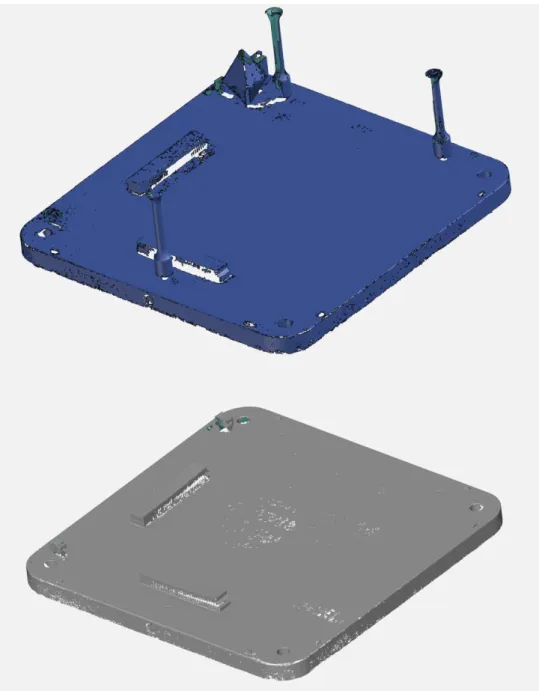
Non-controllable factors are hereby treated as the undesired ones that cannot be eliminated. To minimize them or put them on a known expected interval it is imperative to understand what causes them. Another key aspect worth mentioning is that their effect in this kind of simulation is still not yet completely understood. This has mostly to do with the adaptation that needs to be done to the solver when simulating this process, their constant and continuous changes and all that adding up to the considerable number of controllable factors influence depicted in the previous paragraph. Another reason is the fact that this kind of tools is no yet widespread and is considerably expansive. It was mentioned above that the gas flow inside the chamber can influence the surface finishing of the part. This effect is hard to control but the gas (argon) serves a very important purpose as it is used to prevent ignition inside the building chamber making it impossible to eliminate for safety reasons. Furthermore, the gas flow creates a flux inside the chamber that influences the heat flux through convection (chapter three). Figure 2.6 shows the comparison between a simulated and actual part influenced by the gas flow.

Figure 2.6 Actual part (a) top half; Simulation run (b) bottom half; The colour map was set at the same

scale for both parts and the gas pattern was missed by the simulation. The deviation labels shown are in millimetres

Since the scope of the work is to establish a ground base connection between simulated parts and actual parts, the model was simplified the most and patterns such as the one shown in figure 2.6 are known to exist but were considered to have a minimal effect. Nevertheless, and since it is important to know (especially when considering future work) where they come from an explanation of the possible origin of these patterns is followed.

Some of the variation comes from the different sizes in lose powder, laser beam intensity, wetting and other physical behaviours, and thermal conductivity both in gas and solid materials.

Lose powder

The thermal conductivity of lose powder compares to the conductivity of gas by orders of magnitude smaller than the conductivity in solidified phase [13]. In addition, when considering the intra-particle heat transfer, one can observe that the times scales governing this process are larger than the ones governing particle melting. Under typical SLM process conditions, there is not enough time for conductive homogenization of non-uniform energy and temperature distributions across the powder bed but also across individual particles. As a result, partially molten particles may cause defects such as pores or inclusions [12]. Porosity, as stated above is a very typical undesired output of the SLM process.

Differences in powder grain size can lead to non-uniform energy distributions which may have considerable influence on the resulting melting behaviour and melt pool hydrodynamics yielding hence different temperature fields. The wetting behaviour, liquification of metal (either from different lose powder grain size or hatch pattern) crucially depends on the material, temperature, surface roughness, and surface chemistry. Oxidation is known to considerably decrease the wetting behaviour of the melt which might result in instable, balled melt pools and rough surfaces, pores on delamination due to insufficient layer-to-layer adhesion [14]. The evolution of the solid- phase microstructure characterized by grain size, grain shape (morphology) and grain orientation (texture) are governed by the prevalent spatial temperature gradients, the cooling rates, as well as

Laser Beam Efficiency

Laser beam efficiency is the percentage of laser beam energy that is lost in heat or light during the AM process. Energy from the laser beam (depicted in table 2.3) generates possible energy losses in form of thermal radiation emission, thermal convection or heat conduction from the solidified material to the underlying built platform. Two regimes can be distinguished: 1st _regime

is given by the temperature field in the direct vicinity of the laser beam Heat affected zone (HAZ) [18], which is controlled by highly complex mechanisms such as radiation absorption and heat conduction in the powder bed as well as convective heat transfer within the melt pool with all the individual physical phenomena and process parameters of influence as discussed above. The second regime is prevalent in previously deposited material layers located below the current layer and further away from the heat source. The solidified locations experience repeated heating and cooling cycles with decreasing amplitudes as both the adjacent scan tracks are processed, and consecutive new layers are built. The heat transfer in this regime is rather determined by global part properties.

Geometry

Geometry is controlled by design. Nevertheless, as many AM parts are impossible to build without the use of supports, and there are undesired behaviours when comparing the build orientation and any other orientation, this parameter was developed in this section. Microstructure greatly depends on the specific part geometry, e.g. due to heat flux concentration at the transition region from bulk material to shoulder columns or thin walls, which are surrounded by the low conductivity unfused powder [19, 20].

Furthermore, prevalent length and time scales determine which physical effects govern the process and which are negligible. Typically, viscous and gravity forces can be considered as secondary effects while surface tension and capillary forces, wetting behaviour but also inertia effects are the primary driving forces that influence the metal pool dynamics and shape as well as the surrounding powder morphology by attracting or rejecting individual grains [21]. The heat transfer within the melt pool is governed by convection rather than by heat conduction [22], and material evaporation may also take place [23].

2.4 Context of the Experimental Study

2.4.1 Renishaw AM 250

The machine used to produce the parts for this experiment was a Renishaw AM 250 (Figure 2.7). The name states the maximum power (watts) of the single SLM laser. The machine manufacture is Renishaw. Renishaw is a British company with interests in a variety of areas, but mostly metrology and healthcare. It was founded by Sir David McMurtry that after developing a portable smaller version of a CMM (the Renishaw equator) whilst working for Rolls Royce, decided to patent and develop his idea. Renishaw has a vast experience in the production of 3D parts for healthcare especially dental moulds. Its currently the U.K manufacture and developer on AM machines. AM250 is one of the first being used for metal applications and as had outstanding results. There are currently two other machines from the same manufacturer worth mentioning as they are also being used by HiETA. The Renishaw AM 500 and Renisahw AM 500 ML [24].

Figure 2.7 Ren AM250 a); Ren AM250 Build Chamber b)

Obvious differences between them are the laser power from which their names are taken from. Other than that, an on a more technical aspect the internal powder filter as well as the internal powder feed system are amongst the more significant differences. The trend in the newer versions, as demanded by the market [20] is to have more autonomous and powerful machines and Renishaw’s new releases show exactly that, machines that can work longer and faster with less human intervention. Another significant difference lies on the multi-laser machine (ML) that in Renishaw’s case uses four 500-watt lasers instead of one. This simple aspect of adding three more lasers significantly shortens building time but creates new problems for measuring and simulation tools. Each laser is a source of error and the end individual result from each beam has a different deviation from nominal. Several works are currently being done to eliminate or minimize these sources of deviation.

A continuous adaptation to those changes demanded by market have an intrinsic relation with the motivation of this work.

Furthermore, any given part’s result when fixing all the inputs and varying the machine will change. This is highly related as seen previously to heat behaviour from different hatch types or machine laser power combinations.

2.4.2 Inconel 625

Inconel 625 is a metal superalloy invented in 1962. Its development started in the 50’s to meet the demand for high-strength main stem-line piping material. The typical composition of Inconel alloy 625 is presented in table 2.5.

Table 2.5 Composition of Inconel 625 (%) [25]

The product goals for the development of this new alloy were weldability, high creep resistance, and non-age hardening. From the development of such an alloy another one (Inconel 718 was

Table 2.6 Inconel 625 properties [26]

Property Typical value

Tensile strength 120.00-140.00 (MPa)

Yield strength 60.00-75.00 (MPa)

Elongation 55.00-30.00 (%)

Hardness 145.00-220.00 (MPa)

For this reason, alongside its corrosion resistance under a wide range of temperatures, this alloy is vastly used in AM technologies.

2.4.3 HiETA Technologies

The name stands results from the combination of a word and a letter. High efficiency, the Greek letter ƞ (eta). It emerged from an idea of one of its founders Drummond Hislop on the late 1990’s by realising that a new emerging technology AM would allow new, more efficient architectures for compact heat exchangers whilst looking into ways of improving the performance of the compact heat exchangers on witch Stirling engine depended.

To this day HiETA as in its core research and development to develop and implement novel products in markets such automotive, aerospace, defence, energy and motorsports industry. Although a very young enterprise, it is already regarded as a world-class product development company. The company’s activities almost all lead to carbon reduction with increasing performance of products. Tools such as the one experimented in this work are expected to contribute indirectly to the overall cost reduction enhancing market competitivity [27].

2.5 Thermal Stresses

2.5.1 Basic Definitions

When considering the SLM AM process, three distinct domains of analysis can be set. Table 2.7 synthetises those domains.

Table 2.7 Thermal Domain of analysis in SLM

Domain Description

Macroscopic Component level. Aims to determine residual stresses or dimensional distortion effects

Mesoscopic Detection of defects such as excessive surface roughness, residual porosity or inclusions Microscopic Investigates the metallurgical microstructure

evolution resulting from the high temperature gradients and extreme heating and cooling rates

This work is focused on modelling behaviours at the macroscopic scale. There is an obvious connection between all the domains [28], and although that was considered spatially trough the presentation of the equations of equilibrium, the selected theory that will now be presented had a higher focus on explaining the changes in a macroscopic scale, since the main studied outcome expresses itself in this scale.

Any object contains a certain amount of thermal energy. Thermal energy is the energy contained in the kinetic energy of the random motion of molecules in a body on an atomic level. Temperature is a measure of the averaged kinetic energy of the random particle motion. Only a large number of particles together can have temperature. This property always seeks equilibrium, meaning that the body with higher kinetic energy will hit the particles of the body with lower kinetic energy raising its temperature whilst at the same time reducing its own. This translates by the flow of heat within the body from warmer towards colder parts. Heat can be described as the transfer of thermal energy from one place to another. It only exists as a flow of energy. Hence, to alter the temperature of an object one would need a heat flow. The amount of energy (Joules) required to raise the temperature of the object by one Kelvin is called the object’s heat capacity (Joules/Kelvin). The heat capacity of an object depends on its mass (Kg) and the specific heat capacity of material. Every material has a certain specific capacity [29].

We can consider three fundamental modes of heat transfer depicted in Table 2.8.

Table 2.8 Fundamental modes of heat transfer

Heat Transfer mode Description

Conduction The heat is transferred via molecules vibration. The molecules with a bigger level of vibration transfer some of that kinetic energy to the slower-moving ones

Convection Occurs when a group of molecules with a certain thermal energy is physically moved to another location. Often a flowing liquid absorbs heat from a warmer body and then transports it to a colder body elsewhere

Radiation Emission and absorption of photons. Each photon as a certain energy and that is the energy that is either emitted or absorbed by a given body

SLM process experience all these three fundamental modes of heat transfer. On the one hand, there are variations inside the chamber due to the argon gas flow that will transfer heat via convection. On the other hand, the laser is melting material by raising its temperature to material melting point (molecule vibration) and although this last one is arguably the most significant one of the three [28], there is also radiation present and emitted by the laser. It is this symphony of fundamental heat transfer modes allied with the technology presented in the previous chapter that playfully shapes and deforms the material in the desired formats.

2.5.2 Inherent strains

When particles of a continuous substance move so that distances between particles are changed, the substance is said to be deformed. The concept of deformation is purely geometrical or kinetical and hence independent of the nature of the medium and of the causes of deformation [28].

During SLM thermal-mechanical process, let the deformation be described as 𝑑𝜀𝑖𝑗 consisting

in an element of elastic strain 𝑑𝜀𝑖𝑗𝑒, plastic strain 𝑑𝜀𝑖𝑗 𝑝

, thermal strain 𝑑𝜀𝑖𝑗𝑡ℎ𝑒𝑟𝑚𝑎𝑙 and phase

transformation induced strain 𝑑𝜀_𝑖𝑗𝑝ℎ𝑎𝑠𝑒. As given by the equation 2.1.

𝑑𝜀 = 𝑑𝜀𝑒 _{+ 𝑑𝜀}𝑝 _{+ 𝑑𝜀}𝑡ℎ𝑒𝑟𝑚𝑎𝑙 _{+ 𝑑𝜀}𝑝ℎ𝑎𝑠𝑒 _(2.1)

Once the heating and cooling processes are finished, the residual total strain 𝜀 can be calculated as the summation resulting in equation 2.2.

𝜀 = 𝜀𝑒 _{+ 𝜀}𝑝 _{+ 𝜀}𝑡ℎ𝑒𝑟𝑚𝑎𝑙 _{+ 𝜀}𝑝ℎ𝑎𝑠𝑒 _(2.2)

The inherent strain 𝜀∗ _{is defined by the difference between deformation strain and elastic strain as}

per equation 2.3.

𝜀∗ _{= 𝜀 − 𝜀}𝑒 _(2.3)

The distribution of the inherent strain and residual stress can be assumed to be uniform [32]. Based on this statement and equation 2.3 the calibration principle is explained (see chapter six).

2.5.3 Equations of Equilibrium

Although this experience will not deal directly with the equilibrium equations since the gradients movements are estimated trough the inherent thermal strains the exposure of the equations of movement and the application of the gradient to the heat equation was considered here to provide a better understanding of what the inherent thermal strains are modelling.

In figure 2.8 a parallelepiped used in the determination of the equations of equilibrium is shown.

From it we can define X, Y and Z as the components of the body forces (including inertia forces) in the x, y and z directions respectively. For small displacements such as the ones seen in SLM process we can write equations 3.3.1, 3.3.2 and 3.3.3.

𝑋 = −𝜌 𝜕2𝑢 𝜕𝑡2 𝑌 = −𝜌 𝜕2𝑣 𝜕𝑡2 𝑍 = −𝜌 𝜕2𝑤 𝜕𝑡2 (2.4) (2.5) (2.6)

Where 𝜌 is the mass density, u, v and w are the components of the displacement vector in the x, y and z directions respectively, and t is time.

3

Experimental Setup

This chapter presents both the software simulation principles and the optical scanning measurement system. After introducing the working principles, concepts like voxel and finite elements theory were also investigated. Although closely placed to the border of the scope of this work an explanation as such is necessary to give some clearance on any uncertainty derived from such measuring system.

3.1 Ms Simufact Additive AM

Simufact is a simulating manufacturing software tool with more than twenty years of experience. It is a product from MSC Software, one of the ten original software companies and global leader in simulation software and services. It has been vastly used for other process and industries in the past providing linear and nonlinear finite element analysis (FEA) where 90% of the top manufacturers use MSC software products. The company was founded in 1963 when it was awarded the original contract from NASA to commercialize the FEA software known as NASTRAN (NASA Structural Analysis). MSC has pioneered many of the technologies that are now relied upon by industry analysing and predicting stress, strain, vibration & dynamics, acoustics, and thermal analysis with MSC Nastran [33]. MSC acquired or developed over its history many other well-known computer aided engineer systems (CAE) such as Marc, the one solver in Simufact and used in this experiment. The software’s documentation on previous experiences suggests advantages in both the macro, meso and micro scale approach with better time/detail results to the macro scale.

3.2 Marc Solver

Marc is an advanced nonlinear simulation solver used to simulate responses under static dynamic and multi-physics loading scenarios. Although this experience only looks to the AM build process, the software and the solver can also be used to determine the material behaviour under support removal or heat treatment conditions.

The main variables of a linear FEA analysis are depicted in table 3.1.

Table 3.1 FEA linear analysis variables [34]

Variable Description

Mesh Normally the CAD design without any change. Support

structure can be generated be the software or imported separately

Material Constants Material properties such as strength, ductility and yield point pre-defined on the software

Constraints Constraints used to limit part movement hence limiting rigid body motion

It is important to point out that in a non-linear FEA load increments and non-convergence of runs increase the complexity of the analysis.

The next section of this chapter explains what a voxel is. Nevertheless, the variables presented in table 3.1 are used and linked by the solver trough voxels. The mesh particularly is filled with voxels (voxel mesh) with coordinates whose behaviour (deviation from thermal gradient field) is then followed and simulated.

Whilst the material constants and movement constraints were kept unchanged during this experiment as they are imposed either by design or material specifications, the construction of the mesh and its influence on the result was the subject of this study. The smaller the voxel the highest the level of detail. This affirmation does not always stand has for increasingly short values the noise increases significantly. The change of the voxels size parameter for both the build mesh and the build plate are trying to map a connection between the size values and simulation run time. If the interested pattern on the geometry can be studied with bigger voxels, then the simulation time shortens. Obviously too big of a voxel can generate error from model geometry simplification but defining an acceptable voxel size for a given geometry will also allow the separate import of parts to the software and based on previously determined geometries set different voxel sizes, reducing overall simulation time without compromising accuracy. The origin of the term and fundamental working principle are presented in the following section.

3.3 Voxel

A voxel is a volume element. They are the three-dimensional representation of a pixel. In computers the two main ways of representing graphics are vector and raster. Vectors are a mathematically precise way of describing an image and raster graphics are an array of colour values that are positioned one after the other into a grid pattern [27].

A voxel mesh refers to a mesh that has different number of nodes in neighbouring cell layers (Figure 3.1). This allows the creation of finer resolutions in necessary areas without increasing the number of cells in other areas. Amongst the many advantages is the creation of cells with minimum skewness, automatic mesh generation and uniformity in cell shapes and sizes. The voxel meshes are not yet validated in boundary layer computations. As for disadvantages, it is important to point out that since a voxel as a cube-like shape, the objects representation results in a step like surface of the object (a parallelism between this 3D shape and the raster 2D representation can be made here). The voxel creation utility is embedded in the software and is the central study of this work [35].

algebraic equations over finite volumes (voxels) [36]. The partial differential equations are then discretized/transformed into algebraic equations by integrating them over each discrete element. The system of algebraic equations is then solved to compute the values of the dependent variable for each of the elements. In the finite volume method, some of the terms in the conservation equation are turned into face fluxes and evaluated at the finite volume faces. Because the flux entering a given volume is identical to that leaving the adjacent volume, the FVM is strictly conservative. This inherent conservation property of the FVM makes it the preferred method in computer fluid dynamics (CFD). Two other important aspects of FVM are that it can be formulated in the physical space on unstructured polygonal meshes and the fact that it is quite easy to implement a variety of boundary conditions in a non-invasive manner, since the unknown variables are evaluated at the centroids of the volume elements, not at their boundary faces. In Simufact Additive, the influence of the mesh representation with respect to the real part is determined by a solid fraction. Those elements that are partially filled will have a solid fraction < 1.0 (100%) (E.g. surface elements).

The meshing starts with creating one hexahedral element within the part which has eight gauss points. This one hexahedral element will be subdivided in to eight more hexahedral sub-elements. Control points will be created for all eight sub-elements, figure 3.2. [37].

Figure 3.2 Control points for one voxel [37]

3.4 Simulation Parameters

The software has previously determined parameters for inputs such as material and machine. Before running a simulation, the process, components, manufacturing and analysis widgets need to be completed accordingly. These are the widgets depicted in the top menu of the software in the same order as it is shown in figure 3.3.

Where:

Process – Yellow Component – Orange Manufacturing – Green Analysis – Blue

Each widget parameters inputs influence was considered as per the following paragraphs. The last grey square represents the simulation run widget.

3.4.1 Process

The process widget is where the choices of machine and process are commanded. Table 3.2 shows the options and their description.

Table 3.2 Process widget parameters

Parameter Description

Process type The manufacturing process to be simulated AM machine The software is shipped with pre-set parameters

on AM machines from several manufacturers. The choice of machine is done here

AM build analysis type Choice between Mechanical, Thermal or Thermomechanical analysis.

Type of simulation Manufacturing or Calibration simulation

Manufacturing process stages The selection of processes to simulate is done here.

All the parameters in the process widget were fixed for the experiment at: • Process type - Metal powder bed fusion

• AM Machine - Renishaw AM 250 • AM build analysis type - Mechanical • Type of Simulation - Manufacturing • Manufacturing process stages - Build

3.4.2 Component

It is through the component widget that the part is imported. If the part has a support structure it can be imported here as well or created by the software. Table 3.3 depicts the possible choices on this widget.

Table 3.3 Component widget parameters

Parameter Description

Parts In the parts properties, material properties

such as relative material density can be selected here. Parts dimensions can also be changed here

Supports Can be imported or generated. Similarly, to

parts the relative material density can be select here and the support structure reconfigured

Base Plate Base plate material, dimensions and fixations position are selected here

Material Access to material powder data base and

selection

For the component widget the inputs were: • Part - Ring build CAD

• Support - None (non-existent for the experiment) • Base Plate - 316L_baseplate (Stainless Steel) • Material - IN-625_powder (Inconel 625)

The part was centred on the build plate with the same orientation of the actual builds. Base plate deformation and thickness (15 mm) were selected here, as well as the position and dimension of the bolt holes on the build plate as per the actual process values.

3.4.3 Manufacturing

The parameter allows the selection of the calibrated machine values. The several stages selected on the first widget can be detailed here. In this case we have (table 3.4)

Table 3. 4 Manufacturing widget parameters

Parameter Description

Build Build parameters are defined here. The calibration file from the actual machine is imported here. Machine working inputs such as layer thickness, scan with, start angle and incremental angle are selected here. The post build parameters for this experiment are select here. In this case they refer to the order in which the bolts are extracted from the build plate

Figure 3.4 shows the pop-up window with the options that appear after clinking on the build icon.

Figure 3.4 Build selection menu

The values shown are the ones used in all the experiments that follow, both the experiment and one of the confirmations runs. The second confirmation run did not use the inherent thermal stresses calculation and so the menu changes and is presented in chapter 7.

3.4.4 Analysis

The analysis widget compiles three sub menus depicted in table 3.5

Table 3.5 Analysis widget parameters

Parameter Description

Surface mesh Triangle elements are used to construct the surface mesh. Since the CAD was imported directly to the software, this feature was not changed

Voxel mesh Creation parameters of the hexahedral elements (voxel)

Solver Choice of the number of cores used during the simulation process

Figure 3.5 Meshing properties

Figure 3.5 depicts the parameters that were changed in this experiment they are described in table 3.6.

Table 3.6 Studied variables

Variable Description

Voxel Size The edge length of the voxel element

Minimum fraction for part Allows the specification of the minimum voxel fraction for the part. All voxels with a fraction less than the specified value will be removed from the voxel mesh

Voxel size (Base plate) The edge length of the base plate voxel element

Number of layers (Base Plate) Number of voxel layers over the thickness of the base plate

3.5 Optical Measuring System

An optical measuring system (OMS) is a device that measures the geometry of physical objects via the wave properties of light. The usage of this kind of systems is gradually increasing mostly due to limitations on coordinate measuring machines (CMM), ease of usage and high accuracy [38]. In its basic form, a vision system consists of optical and electronic components to achieve three processes depicted in table 3.7.

Table 3.7 Basic constituents of an Optical Measuring System

Basic Constituent Description

Image Formation and Sensing The object can be illuminated via light transition trough or around itself or by reflecting light. The illuminated object is then imaged to a detector camera, by a suitable optical arrangement

Image Processing After the object has been imaged the resulting mesh needs to be processed by some form of computer or

microprocessor

Communication The final process is to communicate the results of the measurements to the operator. The simplest method is to display graphically the image and measurements on a monitor

Optical measuring process layout can be generally looked up as seen in figure 3.6.

Figure 3.6 Macro image processing system [39]

The layout presented in figure 3.6 is like the one used by the tool used in the experiment. Main difference being that the source of light is incorporated between the lenses. Figure 3.7 shows the operation principle of the gom Scanner.

Figure 3.7 Atos gom scanner [30]

Precise fringe patterns are projected onto the surface of the object and are captured by two cameras based on the stereo camera principle. As the beam paths of both cameras and the projector are known in advance due to calibration, 3D coordinate points from three ray intersections can be calculated. This triple scan principle offers advantages for measuring reflective surfaces and objects with indentations. The result is complete measuring data without holes or erratic points [40].

Working with blue light technology means that interfering ambient light can be filtered out during image acquisition. The light sources are so powerful that measuring date is captured even on non-cooperative surfaces.

As any measuring tool there is an uncertainty associated with the measurements. The sources of uncertainty for the actual measurements taken during the experiment is explained in the next paragraph.

3.6 Measurement uncertainty

The actual parts build for feature acquisition were measured with the gom scan. For this reason, it is important to have an idea of the uncertainty associated with the measurements since the value provided by the measuring equipment was the real or best value of the features.

The measuring system used in the experiment relies on pixel calibration. For this case the uncertainty contributions that apply are the uncertainty form calibration (calibration plate), the pixel calibration value, and the magnification & distortion errors. Other factors that contribute to the overall uncertainty, vary from measurement set to measurement set. They are essentially related to the number of shots taken and room temperature (automatic thermal compensation corrections with an associated uncertainty).

The equipment is calibrated weekly and the data monitored so that all measurements can be related to the external calibration.

External calibration of this equipment set the uncertainty value at

± 1.2 𝜇𝑚 + 2.5 × 𝑙 × 10−6

For k=2 (95% confidence level) Where l is the length (m) measured. The build plate is 250 mm long. But assuming the length to be the perimeter of the outer ring (See chapter 4) with Ø 225 mm, the following is obtained:

Substituting above,

2. 𝜋. 225. 10−3

2 = 0,7068 𝑚

1.2 + 2.5 × 0.7068 = 1.2 µ𝑚

To account for temperature variations, external factors and the overall length of the part measured, the uncertainty considered was ± 2.0 µm.

This rounding value is an overestimate. The best way to determine the uncertainty of an optical measuring system is through a Gauge R&R study. For this reason, to the value calculated in 3.1 a wider interval was considered by rounding the value to next biggest whole number.

4

Experiment Methods

With this chapter the second part of the dissertation begins. In it, the previously stated results from theory are used to set the calibration of the machine. It begins by stating the sequence of the model used for the experiment. It also presents the geometry that was built, the actual measurements and the end of the chapter shows the statistical techniques used through design of experiments.

4.1 Experience Model

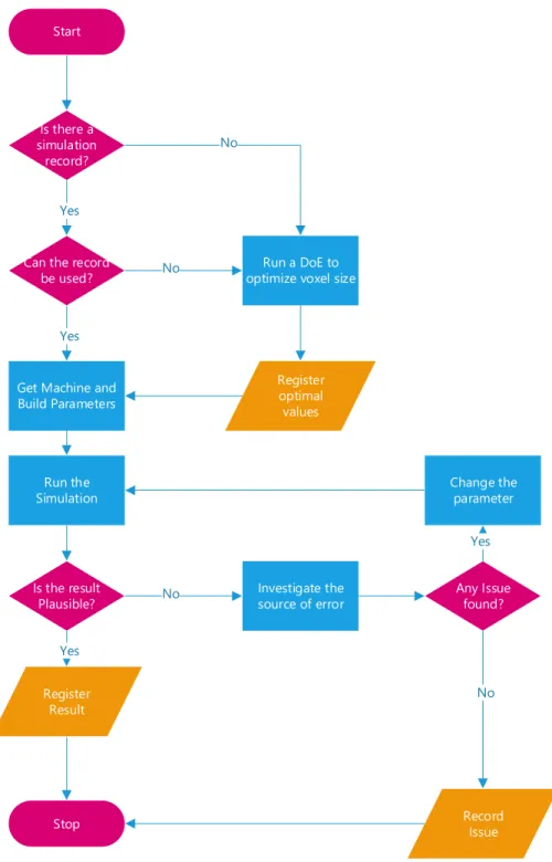
This paragraph describes the model used to conduct the experiment. It was already stated that the software’s capability has never been tested within the company scope completely. For this reason, the starting point was to understand the process functions and significant variance sources. The idealised model that was used in the ring build experiment is depicted in the flowchart shown in figure 4.1. This accounts for the possibility that there is already a previous voxel size shape relation but was built considering also the situation where novel geometries are being tested and for this reason it was used for the experiment.

At the initial stage it is important to register all relevant data that might be used in the future. So, the flowchart presented considers the record both the simulation parameters and statistical analysis in several steps of the way.

The model’s complexity was also kept simple. This was done for the same reason stated above. Since this is an initial draft, simplicity is key to build on further complex models. One of the things that this model doesn’t account is simulations with different voxel sizes trough out the build design. By combining the ideal voxel size of complementary or converging geometries within the same build the simulations times could be greatly reduced.