I
URBAN LAND USE AND LAND COVER CHANGE ANALYSIS AND MODELING A CASE STUDY AREA MALATYA, TURKEY
GÜLENDAM BAYSAL
Dissertation submitted in partial fulfillment of the requirements for the Degree of Master of Science in Geospatial Technologies
II
URBAN LAND USE AND LAND COVER CHANGE ANALYSIS AND MODELING A CASE STUDY AREA MALATYA, TURKEY
Master Thesis by
Gülendam Baysal
Dissertation Supervised by:
Prof. Dr. Edzer J. Pebesma, Institute for Geoinformatics (IFGI), Westfälische Wilhelms-Universität, Münster, Germany.
Dissertation Co-Supervised by:
Prof. Dr. Jorge Mateu M., Department of Mathematics, Universitat Jaume I (UJI), Castellon, Spain.
Prof. Dr. Pedro Cabral, Instituto Superior de Estatística e Gestão de Informação (ISEGI), Universidade Nova de Lisboa, Lisbon, Portugal.
III
DECLARATION OF ORIGINALITY
I declare that the submitted work is entirely my own and not belongs to any other person. All references, including citation of published and unpublished sources have been appropriately acknowledged in the work. I further declare that the work has not been submitted for the purpose of academic examination, either in its original or similar form, anywhere else.
Münster, 28th February, 2013
Gülendam Baysal
IV
ABSTRACT
This research was conducted to analyze the land use and land cover changes and to model the changes for the case study area Malatya, Turkey. The first step of the study was acquisition of multi temporal data in order to detect the changes over the time. For this purpose satellite images (Landsat 1990-2000-2010) have been used. In order to acquire data from satellite images object oriented image classification method have been used. To observe the success of the classification accuracy assessment has been done by comparing the control points with the classification results and measured with kappa. According to results of accuracy assessment the overall kappa value found around 75%. The second step was to perform the suitability analysis for the urban category to use in modeling process and it has been done using the Multi Criteria Evaluation method. The third step was to observe the changes between the defined years in the study area. In order to observe the changes land use/cover maps belongs to different years compared with cross tabulation and overlay methods, according to the results it has been observed that the main changes in the study area were the transformation of agricultural lands and orchards to urban areas. Every ten years around 1000ha area of agricultural land and orchards were transformed to urban. After detecting the changes in the study area simulation for the future has been performed. For the simulation two different methods have been used which are; the combination of Cellular Automata and Markov Chain methods and the combination of Multilayer Perceptron and Markov Chain methods with the support of the suitability analysis. In order to validate the models; both of them has been used to simulate the year 2010 land categories using the 1990 and 2000 data. Simulation results compared with the existing 2010 map for the accuracy assessment (validation). For accuracy assessment the quantity and allocation based disagreements and location and quantity based kappa agreements has been calculated. According to the results it has been observed that the combination of Multilayer Perceptron and Markov Chain methods had a higher accuracy in overall, so that this combination used for predicting the year 2020 land categories in the study area. According to the result of simulation it has been found that; the urban area would increase 1575ha in total and ~936ha of agricultural lands and orchards would be transformed to the urban area if the existing trend continued.
Key words: Land Use, Land Cover, Remote sensing, GIS, Cellular Automata,
V
ACKNOWLEDGEMENT
I would like to express my gratitude to all those who gave me the possibility to complete this thesis. First of all I want to thank to my family for their moral support, encouragement and care.
I also want to thank my supervisors Prof. Dr. Edzer J. Pebesma, Prof. Dr. Jorge Mateu M., Prof. Dr. Pedro Cabral for their comments and suggestions. Moreover I would thank to Federal Ministry of Innovation, Science and Research of North Rhine-Westphalia for funding my study.
Special thanks to Firat Development Agency for providing the data and special thanks to my friends Dilşat Kazazoğlu Temiz, expert at Firat Development Agency, and Özge Öztürk, GIS specialist at Ministry of Agriculture, for assisting me while collecting the data for my thesis and for their moral support.
Special thanks to Dr. Christoph Brox, Prof. Dr. Werner Kuhn, Prof. Dr. Christian Kray for their comments during my studies on my thesis. Furthermore I want to thank to Professor Robert Gilmore Pontius Jr., Clark University, for his suggestions and sharing the useful sources.
Finally many thanks to my classmates from all over the world for sharing their knowledge and for their moral support.
VI
ACRONYMS
ANN: Artificial Neural Network CA: Cellular Automata
ED: European Datum
ETM: Enhanced Thematic Mapper FDA: Firat Development Agency LULC: Land Use Land Cover MARKOV: Markov Chain Model MCE: Multi Criteria Evaluation MLP: Multilayer Perceptron TM: Thematic Mapper
USGS: U.S Geological Survey
UTM: Universal Transverse Mercator WGS: World Geodetic System
WLC: Weighted Linear Combination TurkStat: Turkish Statistical Institute
VII
INDEX OF CONTENT
DECLARATION OF ORIGINALITY ... III ABSTRACT ... IV ACKNOWLEDGEMENT ... V ACRONYMS ... VI INDEX OF CONTENT ... VII INDEX OF FIGURES ... IX INDEX OF TABLES ... X
1 INTRODUCTION ... 1
1.1 Background and Motivation ... 1
1.2 Study Area ... 1
1.3 Statement of the Problem ... 2
1.4 Objectives ... 2
1.5 Research Questions ... 3
1.6 Theoretical Background and Basic Terminologies ... 3
1.7 Previous Studies ... 4
1.8 Structure of Thesis ... 4
2 METHODOLOGY AND DATA ... 6
2.1 Methodology ... 6
2.1.1 Image Classification ... 6
2.1.2 Suitability Analysis ... 7
2.1.3 Change Detection and Modeling ... 7
2.2 Multi Temporal and Multispectral Data (Landsat Images) ... 8
2.3 Other Data Sources ... 9
2.4 Tools ... 9
2.5 Study Area Selection ... 10
2.6 Data Preprocessing ... 10
3 IMAGE CLASSIFICATION ... 11
3.1 Pixel Based Classification ... 11
3.1.1 Supervised Classification ... 11
3.1.2 Implementation of Supervised Classification for Study Area ... 15
3.2 Object-oriented Image Segmentation and Classification ... 17
3.2.1 Watershed Delineation Segmentation ... 17
3.3 Accuracy Assessment ... 19
4 SUITABILITY ANALYSIS ... 20
4.1 Multi Criteria Evaluation ... 20
4.1.1 Weighted Linear Combination ... 21
VIII
4.1.3 Weight Decision ... 22
4.1.4 Implementation of Suitability Analysis ... 22
4.2 Suitability Analysis Results ... 29
5 CHANGE DETECTION ANALYSIS ... 30
5.1 Changes between 1990-2000 ... 30
5.2 Changes between 2000 -2010 ... 32
6 LAND USE AND LAND COVER CHANGE MODELING ... 35
6.1 Cellular Automata and Markov Chain ... 35
6.1.1 Markov Chain ... 35
6.1.2 Cellular Automata ... 37
6.1.3 Combination of Cellular Automata and Markov Chain Methods ... 39
6.2 Multilayer Perceptron and Markov Chain ... 41
6.2.1 Artificial Neural Networks ... 41
6.2.2 Multilayer Perceptron ... 42
6.2.3 Combination of Multilayer Perceptron and Markov Chain Methods ... 43
6.3 Accuracy Assessment ... 46
6.3.1 Quantity and Allocation Disagreements ... 48
6.3.2 Kappa ... 48
6.4 Simulation for the Year 2020... 50
6.4.1 Changes Based on Simulated 2020 Map (2010-2020) ... 52
7 DISCUSSION AND CONCLUSION ... 53
7.1 Limitation of the Research ... 54
7.2 Recommendations... 54 REFERENCES ... 55 APPENDIX A ... 60 APPENDIX B ... 63 APPENDIX C ... 64 APPENDIX D ... 65
IX
INDEX OF FIGURES
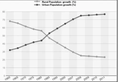
Figure 1-1: Urban and rural population growth rate (%) for Turkey (TurkStat, n.d.) ... 1
Figure 1-2: Location of study area ... 2
Figure 2-1 : Image classification workflow ... 6
Figure 2-2 : Suitability analysis workflow ... 7
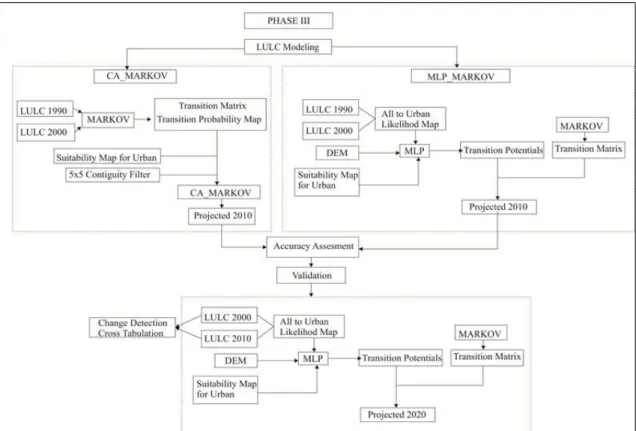
Figure 2-3 : Change detection and simulation workflow ... 7
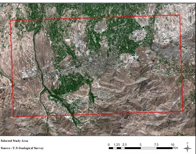
Figure 2-4: Study Area ... 10
Figure 3-1: Classic supervised classifiers (Caetano, 2009)... 12
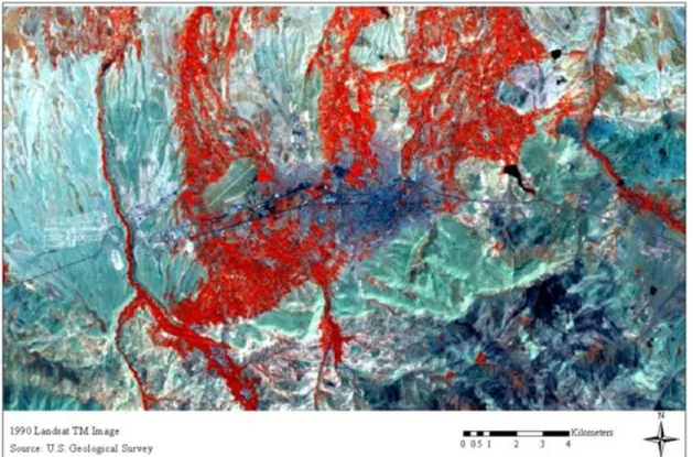
Figure 3-2: Study area profile with Landsat image (1990) ... 13
Figure 3-3: Study area profile with Landsat image (2000) ... 13
Figure 3-4: Study area profile with Landsat image (2010) ... 14
Figure 3-5: Development of training sites ... 14
Figure 3-6: Pixel based classification result (1990) ... 16
Figure 3-7: Pixel based classification result (2000) ... 16
Figure 3-8: Pixel based classification result (2010) ... 16
Figure 3-9: Object based Classification (Caetano, 2009) ... 17
Figure 3-10: Segmentation based classification result (1990) ... 18
Figure 3-11: Segmentation based classification result (2000) ... 18
Figure 3-12: Segmentation based classification result (2010) ... 18
Figure 4-1: Linear membership functions (Eastman, 2009) ... 22
Figure 4-2: Constrains ... 23
Figure 4-3: Urban area boundary changes ... 25
Figure 4-4: Road & urban relation ... 25
Figure 4-5: Trend chart for road & urban relation ... 26
Figure 4-6 : Standardized factors ... 27
Figure 4-7: Urban suitability ... 29
Figure 5-1: Gains and losses in each class (1990 - 2000) ... 30
Figure 5-2: Transition from other categories to urban (1990-2000) ... 31
Figure 5-3 : Contribution from other categories to orchard (1990-2000) ... 32
Figure 5-4 : Contribution from other categories to agriculture (1990-2000) ... 32
Figure 5-5: Gains and losses in each class (2000- 2010) ... 32
Figure 5-6: Transition from other categories to urban (2000-2010) ... 33
Figure 5-7: Contribution from other categories to orchard (2000-2010) ... 34
Figure 5-8: Contribution from other categories to agriculture (2000-2010) ... 34
Figure 6-1: Markov conditional probability images ... 37
Figure 6-2: Contiguity filter (5X5) ... 39
Figure 6-3: Suitability maps for other classes ... 40
Figure 6-4: Image classification result for 2010 LULC map ... 40
Figure 6-5: Projected LULC for 2010 (CA and MARKOV) ... 41
Figure 6-6: ANN structure (Artificial Neural Networks, n.d.) ... 42
Figure 6-7: Back propagation ... 42
Figure 6-8: Likelihood ... 43
Figure 6-9: Digital elevation model ... 44
Figure 6-10: Image classification result for 2010 LULC map ... 45
Figure 6-11: Projected LULC for 2010 (MLP and MARKOV) ... 45
Figure 6-12: Prediction correctness and error based on 2000 (reference), the 2010 (reference) and 2010 (simulation result of CA and MARKOV) LULC maps ... 46
Figure 6-13: Prediction correctness and error based on 2000 (reference), 2010 (reference) and 2010 (simulation result of MLP and MARKOV) LULC maps ... 47
X
Figure 6-14: Likelihood ... 50
Figure 6-15 : Simulation for the 2020 ... 51
Figure 6-16 : Gains and losses in each category (2010-2020) ... 52
Figure B-0-1: CORINE 1990 ... 63
Figure B-0-2: CORINE 2000 ... 63
Figure B-0-3: CORINE 2006 ... 63
INDEX OF TABLES
Table 1-1: Urban and rural populations in 1965 (TurkStat, n.d.) ... 2Table 1-2: Urban and rural populations in 2011 (TurkStat, n.d.) ... 2
Table 1-3: Literature review on the LULC change models ... 5
Table 2-1 : Landsat images basic properties ... 8
Table 2-2 : Landsat TM image properties ... 8
Table 2-3 : Landsat ETM+ image properties ... 8
Table 3-1 : LULC categories (CORINE land cover technical guidelines, 2000) ... 15
Table 4-1: Continuous Rating Scale ... 22
Table 4-2 : Pairwise comparison matrix ... 28
Table 4-3: Weight of Factors ... 28
Table 5-1: Transition from other categories to urban (1990-2000) ... 31
Table 5-2: Transition from other categories to urban (2000-2010) ... 33
Table 6-1: Markov Chain variables ... 36
Table 6-2: Markov conditional probability of changing among LULC type ... 36
Table 6-3: Cells expected to be transformed to other classes ... 36
Table 6-4: Cramer’s V for each variable (2010) ... 44
Table 6-5: Components of agreement and disagreement for the combination of CA and MARKOV methods results ... 48
Table 6-6: Components of agreement and disagreement for the combination of MLP and MARKOV methods results ... 48
Table 6-7: Accuracy assessment (CA and MARKOV) ... 49
Table 6-8: Accuracy assessment (MLP and MARKOV) ... 49
Table 6-9: Cramer’s V for each variable (2020) ... 50
Table 6-10: Markov conditional probability of changing among LULC types ... 51
Table 6-11: Cells expected to be transformed into other classes ... 51
Table 6-12 : Transitions from each category to urban ... 52
Table A-0-1: Sample error matrix ... 60
Table A-0-2: 1990 Error matrix and accuracy values ... 61
Table A-0-3: 2000 Error matrix and accuracy values ... 61
Table A-0-4: 2010 Error Matrix and Accuracy Values... 62
Table C-0-1: Questionnaire forms filled by experts for suitability analysis ... 64
Table D-0-1: Cross tabulation results of the combination of Cellular Automata and Markov Chain methods ... 65
Table D-0-2: Cross tabulation Results of the combination of Multilayer perceptron and Markov Chain methods ... 65
1
1 INTRODUCTION
1.1 Background and Motivation
Land use and land cover changes are dynamic spatial issues and in order to have a sustainable development these changes need to balanced. In many cities this balance spoiled because of rapid population growth in urban areas. The main increase in urban population results by rural to urban migration. In Turkey mass movements from rural to urban has increased after the 1960s and especially after 1990s the increase rate gained a momentum, from figure 1-1 urban and rural population growth rate can be observed.
Figure 1-1: Urban and rural population growth rate (%) for Turkey (TurkStat, n.d.)
The growth in the urban population caused the transformation of the agricultural lands on the outskirts of the cities to the urban area. For a sustainable development the transformations need to be balanced, but for many cities in Turkey it was not balanced. Controlling the changes can be managed by planning authorities in order to lead them many researches worked on the land change modeling issues.
1.2 Study Area
Malatya is located at 38°21′N 38°18′E on the East Anatolian Region of Turkey, the city is best known for its apricot orchards. The location of the city is important because it is on the trade ways from east to west (figure 1-2). The population characteristic of Turkey and the Malatya can be observed in the table 1-1 and 1-2. As we can see from the tables the urban population in the study area tripled in 46 years
2
whereas the rural population decreased %50 percent. As a result of this population increase a demand for housing increased.
Table 1-1: Urban and rural populations in 1965 (TurkStat, n.d.)
Year 1965 Total Urban Rural
Turkey 31,391,421 10,805,817 20,585,604
Malatya 452,624 147,040 305,584
Table 1-2: Urban and rural populations in 2011 (TurkStat, n.d.)
Year 2011 Total Urban Rural
Turkey 74,724,269 57,385,706 17,338,563
Malatya 740,643 480,144 260,499
Figure 1-2: Location of study area
1.3 Statement of the Problem
After 1965 the study area started to gain migration because of having more job opportunities and services. Until 1990s this movement was not critical but after that the population of the city increased rapidly, because it became a pole of attraction for the surrounding regions (Ünal, 2010). However the city was not ready for this migration; there was not enough housing for the new population. In the beginning people started to settle down on the outskirts of the city, in farmhouses which are not affecting the agricultural lands. Nevertheless in recent years this has changed and instead of farm houses 7-10 storied apartments raised. The main problem of the study area is unbalanced growth in urban area which means the growth urban area affected the agricultural lands on the outskirts of the city. Since the city has important agricultural sources like apricot orchards in the periphery, this transformation need to be monitored.
1.4 Objectives
The main aim of the study is to understand the urban area changes and the transformations from other land categories to urban area and the main objective of
3
the study using geospatial tools and techniques for monitoring the changes and then modeling the future land classes. According to this aims and objectives we can list main steps of the study as;
Creating LULC maps from satellite images by image classification techniques (1990-2000-2010).
Comparing the results of classification with reliable sources (CORINE, STATIP and Google Earth) for the accuracy assessment.
Using the LULC categories for the years 1990-2000 and 2000-2010 to detect the changes in the study area.
Using the LULC categories for the years 1990-2000 to simulate the year 2010 in order to validate the model.
If the model is useful for the study area the simulating the LULC categories for the year 2020.
1.5 Research Questions
Are the available data adequate for this study?
Are GIS and remote sensing tools adequate for this study?
Can the mathematical models help to model LULC changes?
Where are the main changes and where is the main growth direction of the urban area according to simulated result for the year 2020?
1.6 Theoretical Background and Basic Terminologies
In order to understand the LULC changes it is important to know about the tools and models for change detection and simulation. GIS and remote sensing tools and mathematical models are the main components of the change detection and simulation. In this section we try to summarize the main concepts mentioned in the study.
“Remote sensing is the acquisition of information about an object or phenomenon without making physical contact with the object.”” (Schowengerdt, 2006). Remote sensing is the primary sourcing of multispectral and multi temporal data which will help us to detect the changes.
“Geographic Information System (GIS) is a system designed to capture, store, manipulate, analyze, manage, and present all types of geographical data” Geographic information system (n.d.).The power of GIS could help us to process the data and make analysis on the data.
“A mathematical model is a description of a system using mathematical concepts and languages” (Mathematical Model, n.d.). The mathematical models help us to understand the system and then by understanding the system behaviors it helps us to predict the future.
4
Land use is related how the land is used, how the natural environment changes to
human built up area. Land cover is physical cover of the surface of the earth not related human activities it is natural. (García, Feliú, Esteve, Soba, Hazeu, Rasmussen, Galera-Limdblom & Banski 2010)
1.7 Previous Studies
Many researchers worked on LULC change modeling, with different methodologies and techniques. The table 1-3 prepared in order to summarize some of the works and models which can be implemented in LULC change modeling. Every model has different data requirements, strengths and weaknesses. For this research mainly two approach has been implemented which are combination of Cellular Automata and Markov Chain methods and the combination of Multilayer Perceptron and Markov Chain methods, because of the data availability and the aim of the research.
1.8 Structure of Thesis
The thesis divided into seven chapters in order to explain the each step of the study in detail. In the first chapter the background of the research, study area, the statement of the problem, objectives, research questions, previous studies explained and the main terminologies defined. The second chapter is including the methodology and the data used for the study. Third chapter explains the first phase of the study which is image classification. The fourth chapter deals with the suitability analysis for the urban area which has been used in the modeling part of the study. Fifth chapter explains the changes between the years 1990 -2000 and 2000-2010 in order to investigate the major changes in the study area. Sixth chapter explains the LULC modeling with two different models which are combination of CA and MARKOV methods and the combination of the MLP and MARKOV methods moreover it includes the model validation step and with the accuracy assessment and simulation of the LULC for the year 2020.
5
Table 1-3: Literature review on the LULC change models
Model Name Builder Model Type What it Explains Variables Strengths Weakness
(Agarwal et al., 2002)
Markov Model Wood et al. 1997
Spatial Markov model
Landuse change Multi Temporal Land Use/ cover maps
Considers both spatial and temporal change No sense of Geography (Agarwal et al., 2002) CA Clarke et al. 1998; Kirtland et al. 2000 Cellular Automata model
Change in urban areas over time
Extent of urban areas, Elevation, Slope, Roads
Allows each cell to act independently according to rules
Doesn't include human and biological factors (Adhikari & Southworth, 2012 ) Combination of CA and MARKOV methods
Clark Labs Spatio-Temporal
dynamic modeling
Predicts land use/cover in the future
Multi Temporal Land Use/ cover maps, Suitability maps
Creating the Data is easy, CA add spatial dimension to the model, can simulate change among several categories
Socio economic factors are not
considered , Calibarting the model with MCE is too much time consuming compared to other methods (Agarwal et
al., 2002)
UrbanSim Paul Waddell (University of California, Berkeley)
Cellular Automata and individual based model
Spatial maps of housing units by pixel,
nonresidential square footage per cell and other economic and
demographic characteristics
Parcel files, business
establishment files census micro data, Environmental, political, and planning boundaries, location grid control totals from economic regional forecasts, travel access indicators, scenario policy assumptions
Structure allows multiple types of policies to be explored High degree of precision, Employment locations modeled, Designed to provide inputs to the transportation demand model
High data demands, designed for urban areas
hard to understand the model, It has rigid model structure, Output must be
imported into GIS for viewing
(Li & Yeh, 2002)
Combination of ANN and CA methods
Antony Gar-On Yeh, Xia Li
ANN & Cellular Automata Model
Predicts land selected land class in the future
Multi Temporal Land Use/ cover maps
Calibrating the model with ANN It can simulate change only in two category
(Pontius & Chen, 2008)
GEOMOD Clark Labs Cellular Automata Predicts land selected
land class in the future
Land use/cover map Need only one time land use map for calibration
It can simulate change only in two category
(Torrens, 2000) (Agarwal et al., 2002)
SLEUTH Dr. Keith C. Clarke at UCSanta Barbara
Spatially explicit Cellular Automata model
GIS maps of probability (continuous) of
urbanization in a specified pixel
Multi Temporal Land Use Map, Impervious surface cover , Road networks (for each time period), Slope (%), Undevelopable land
Relatively easy to transfer among regions,
incorporate many different land use classifications systems ,it generates
continuous measure of density of
development , take into consideration the
future developments (such as road) Designed for urban settings, Data
demands are high, Un-calibrated model would produce more
error ,Difficult to use
Land Change Modeler Clark Labs Markov Chain ,
MLP, Logistic Regression , SimWeight
Change Analysis , Predicts land use/cover in the future
Land Use Land Cover data, Road ,DEM, Other Infrastructure
Environmental modeling platform, taking into consideration the future projects, Using the ANN for development of transition potentials, calculating the changes in two time periods
Consideration of one sub model
(Agarwal et al., 2002)
CLUE (Conversion of Land Use and Its Effects)
(Veldkamp and Fresco 1996a)
Discrete, finite state model
Predicts land use/cover in the future
Land suitability for crops,
Temperature/Precipitation, Effects of past land use, Impact of pests, weeds, diseases, Human Drivers, Population size and density, Technology level, Level of affluence, Political Structures, Economic conditions, Attitudes and values
Covers a wide range of biophysical and human drivers at differing temporal and spatial
scales
Limited consideration of institutional and economic variables (Agarwal et al., 2002) LUCAS (Landuse Change Analysis System)
Michael Berry, Richard Flamm, Brett Hazen, Rhonda MacIntyre, and Karen Minser; University of Tennessee
Spatial stochastic model
Transition probability matrix, landscape change. Assesses the, impact on species habitat.
Land cover type, Slope, Aspect, Elevation,
Land ownership, Population Density, Distance to nearest road, Distance to nearest economic market, center, Age of trees
Model shows process , output (new land use map), and impact (on species habitat)
LUCAS tended to fragment the landscape for low proportion land uses, due to the pixel based independent grid
method. Patch based simulation would cause less fragmentation, but patch definition requirements often lead to their degeneration into one cell patches
6
2 METHODOLOGY AND DATA
2.1 Methodology
The methodology of the research composed of three phases.
Image Classification
Suitability Analysis
Change detection and Modeling the LULC
2.1.1 Image Classification
The first phase of the study was acquiring the land use/cover classes from remote sensing sources by classification methods. In figure 2-1 the classification workflow illustrated for summarizing the general outline of this phase. The details have been explained in chapter three.
7
2.1.2 Suitability Analysis
Second phase of the study was the suitability analysis for the urban development. In figure 2-2 the schema of the suitability analysis using the multiple criteria evaluation method conceptualized. In chapter four the details of the work can be found.
Figure 2-2 : Suitability analysis workflow
2.1.3 Change Detection and Modeling
The third phase of the research was change detection and future prediction. In figure 2-3 this workflow of this phase can be observed. The details for change detection were explained in chapter five and modeling was explained in chapter six.
8
2.2 Multi Temporal and Multispectral Data (Landsat Images)
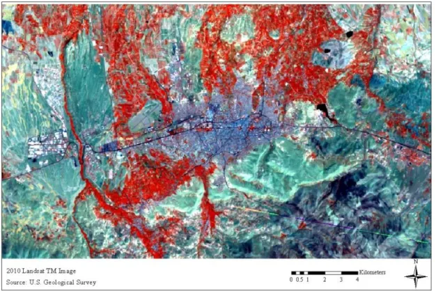
For the land change detection and modeling the initial step is the data acquisition and the most common sources are the remote sensing sources, because the acquisition of the vector data is expensive and time consuming, finding the multi temporal data in order to detect the changes is not easy, especially in developing countries. For the study area the multi temporal vector data was CORINE which was prepared in 25 ha minimum mapping unit. But this resolution was not detailed enough because of that satellite images have been used. The summer period Landsat images selected for preparation of land use/cover data. The reason of using the summer period was to distinguish the other agriculture from orchards and to observe the transformation from urban area to these classes separately. In order to have better accuracy in classification the cloud free Landsat images used; for this reason in the year 1990 the month for the image is June and the sensor is ETM+ and for 2000 and 2010 the month is July and the sensor is TM. The properties of the images can be found in table 2-1, 2-2 and 2-3.
Table 2-1 : Landsat images basic properties
Date Date Acquired Spacecraft ID Sensor ID
1990 12-Jun-90 LANDSAT_5 "TM"
2000 17-Jul-00 LANDSAT_7 "ETM"
2010 5-Jul-10 LANDSAT_5 "TM"
Table 2-2 : Landsat TM image properties
Landsat 5 (TM sensor) Wavelength (micrometers) Resolution (meters)
Band 1 0.45 - 0.52 30 Band 2 0.52 - 0.60 30 Band 3 0.63 - 0.69 30 Band 4 0.76 - 0.90 30 Band 5 1.55 - 1.75 30 Band 6 10.40 - 12.50 120 Band 7 2.08 - 2.35 30
Table 2-3 : Landsat ETM+ image properties
Landsat 7 (ETM+ sensor) Wavelength (micrometers) Resolution (meters)
Band 1 0.45 - 0.515 30 Band 2 0.525 - 0.605 30 Band 3 0.63 - 0.69 30 Band 4 0.75 - 0.90 30 Band 5 1.55 - 1.75 30 Band 6 10.40 - 12.5 60 Band 7 2.09 - 2.35 30 Pan Band .52 - .90 15
9
2.3 Other Data Sources
The LULC changes can be predicted using the multi temporal land use/cover data but also other data sources needed for the improvement of the study. For this purpose other data related to the study area has been collected from the Firat Development Agency (they have been prepared by different institutions) and processed with GIS software. The other data sources are;
Roads: Main road network of the study area prepared by Ministry of Transportation in national level.
Water bodies: Lakes and dams in the study area prepared by Turkey General Directorate of State Hydraulic Works.
Protection Areas and: These are including the naturally protected and it has been prepared by Ministry of Culture and Tourism.
Archeological Areas: These areas are approved archeological zones and also prepared by Ministry of Culture and Tourism
STATIP (Problem Identification and Improvement of Agricultural Lands Project): This data is including the main land cover map for the year 2008 which prepared by Ministry of Agriculture of Turkey for identification of problematic agricultural lands, because of this it is mainly concentrated on agricultural lands. The data has been prepared using the SPOT 5 images with 2.5 and 5m resolution.
CORINE (Coordination of Information on the Environment prepared by the European Environmental Agency): This data includes the main land cover maps with 25 ha minimum mapping unit.
Approved Development Plan: This data is including the approved development plan for the study area prepared by municipality of the study area in the year 2009.
DEM: Digital elevation model for the study area (30m resolution).
2.4 Tools
The tools have been used for the study varies, main tools used for the development of the research are;
ArcGIS 10 used for image and vector data preprocessing.
IDRISI Selva* used for classification, accuracy assessment of classification, change detection and modeling.
ENVI** used for testing some other classification methods.
Map Comparison Kit 3*** used for accuracy assessment of the projected land classes.
*IDRIS Selva is a GIS and remote sensing software. **ENVI is remote sensing software.
10
2.5 Study Area Selection
The study area was defined in order to investigate the changes in the urban area and the outskirts of the urban area. For this purpose bounding box which covers these focus areas covering an area of 40612 ha area has been used (figure 2-4).
Figure 2-4: Study Area
2.6 Data Preprocessing
The Landsat images were covering a large area (3500000 ha) but for this research the study area was just 40612 ha, because of that Landsat images were clipped according to the bounding box which covers the study area. Moreover Landsat images were in GeoTIFF* format in order to use them in different software especially in IDRISI images have been exported to ERDAS IMAGINE** format. Finally the Vector data received from Firat Development agency was in ED_1950 system, so these data have been transformed to the WGS_84 system in order to be same with Landsat images which are in WGS_84 system and then clipped according to the study area.
*GeoTIFF is a public domain metadata standard which allows georeferencing information to be embedded within a TIFF (image) file (GeoTIFF, n.d.).
11
3 IMAGE CLASSIFICATION
For land change analysis and modeling the first step is the land use/cover data preparation. Land categories can be acquired by the classifying satellite images. Images are including the color differences, these colors are not the real land classes, in order to get the real category information from the bands the images need to be classified. Image classification is the process of categorizing image pixels into classes to produce a thematic representation (Gecena & Sarpb, 2008). There are several methods for classification and each method is specific to the data and the location, because in each location land categories are varies and have different values in the image. For instance the image value (reflectance) of an agricultural land is dependent on the type of crop grows on that land. Even the same crop in different climates can have different colors which change the color on the image. Moreover the seasons also affect the color of land covers.
There are different approaches for classification. According to Caetano (2009) Image classification can be done based on three objectives which are;
Type of learning (Supervised and Unsupervised)
Assumptions on data distribution (Parametric, Non-Parametric)
Number of outputs for each spatial unit (Hard and Soft) (Caetano, 2009) Moreover there are also objectives regarded levels of classification, which are;
Pixel based Classification
Object-oriented Image Segmentation and Classification
3.1 Pixel Based Classification
Pixel based classification is the traditional method of image classification. This is mainly based on the pixel reflectance values of the image (Wang, Sousa & Gong, 2004). According to the type of learning there are mainly two kinds of pixel based classification supervised and unsupervised (Caetano, 2009). For this study the supervised method used for the pixel based classification.
3.1.1 Supervised Classification
“Supervised classification is a procedure for identifying spectrally similar areas on an image by identifying “training” sites of known targets and then extrapolating those spectral signatures to other areas of unknown targets” (Mather & Koch, 2011 ).
As we can understand from the definition in supervised classification there is a priori knowledge about the image so the image will be classified according to this prior knowledge which is called training sites. Training sites are the areas for which the characteristics are known according to a ground truth or other reliable data. Here the ground truth refers to the data collected from the ground (Ground Truth, n.d.).
12
Figure 3-1: Classic supervised classifiers (Caetano, 2009)
There are different algorithms for supervised classification; the classic classifiers are minimum distance, parallel pipelined and maximum likelihood methods. As it can be observed from the figure 3-1 each of these classifiers uses different statistical approaches for the classification, for this research the maximum likelihood used because it gave better results for the study area.
3.1.1.1 Maximum Likelihood Algorithm
The maximum likelihood algorithm uses a maximum likelihood procedure derived from Bayesian probability theory; it applies the probability theory to the classification process. This method is a supervised method which uses the training sites, from these sites it determines the class center and the variability in the raster values in each band for each class. This will help to determine the probability of the cell to be belonging to a particular class defined in training sites. The probability is depending on distance from cell to class center, as it has been illustrated in figure 3-1, class size and the shape of the class in spectral space. The maximum likelihood classifier computes the class probabilities and classifies the cell where the probability is higher (Smith, 2011).
3.1.1.2 Image Enhancement
There are different image enhancements methods are available for images which helps to acquire the category information from the image. Histogram modification, filtering and band compositions are some of the methods. For this research band composition method has been implemented. Each band composition algorithm enhances the different category information from the images. For this study false color composition used which is a combination of VNIR (Visible Near Infra-Red) (4) - red (3) - green (2) in which vegetation seems as red tones, urban areas appear blue towards to gray , water appears blue (Band Combinations, n.d.). Using this composite will help to distinguish between the orchards and other agricultural lands easily and which is one of the objectives of the research. For distinguishing urban area is difficult with any of the composite method, because the urban area of the case study include composed of mixed pixels. Still compared to the other compositions false color composition is the best choice for the study area. The Landsat images for the study area can be observed in figure 3-2, 3-3, 3-4.
13
Figure 3-2: Study area profile with Landsat image (1990)
14
Figure 3-4: Study area profile with Landsat image (2010)
3.1.1.3 Developing the Training Sites
As it has been mentioned before in the supervised classification training sites need to be used as a priori knowledge. For the study are ground truth data is not available for this reason CORINE, STATIP and user interpretation from the satellite image used for development of the training sites. Around 250 training sites selected for the each image the category information for this sites acquired from CORINE and STATIP datasets tested with the user interpretation. For the year 2010 CORINE is not available because of this reason CORINE 2006 and Google earth used for defining the training sites (figure 3-5).
15
3.1.2 Implementation of Supervised Classification for Study Area
The LULC categories determined according to the objectives of the research in which urban areas, orchards, other agricultural lands, other land cover categories and water body are the main groups. While defining this group’s structure in CORINE project used. CORINE has almost 32 categories but for the study area they generalized to 5 main classes as it can be observed from table 3-1. The main research objective of this study was to find the change in urban areas and agricultural usages (agriculture and orchard) and modeling them because of that the classes different than them generalized to other. Water bodies haven’t been added to this other class because the reflectance value of the water is not similar to other class.
Table 3-1 : LULC categories (CORINE land cover technical guidelines, 2000) Generalized Class Classes from CORINE
Agriculture Irrigated Agriculture , not irrigated agriculture, principally agricultural lands in which some parts covered by natural vegetation, vineyards Orchard Irrigated orchards, not irrigated orchards
Urban
Construction sites, Industrial and Commercial Units, Continuous Urban Fabric, Non continuous Urban Fabric, Continuous and non-continuous Rural Fabric, Airports, Roads Railways, Mineral extraction Sites, Green Urban Areas
Other Sparsely Vegetated Areas and Transitional Woodland Shrub, Natural Grassland , Pastures, Sand dunes, Inland Marshes
Water Dams , lakes
In order to use the supervised classification the training samples were created based on reliable sources, then the supervised classification based on maximum likelihood algorithm has been used for classification because the other algorithms result was not satisfactory. The results of the pixel based classification can be observed in the figures 3-6, 3-7, 3-8.
16
Figure 3-6: Pixel based classification result (1990)
Figure 3-7: Pixel based classification result (2000)
17
3.2 Object-oriented Image Segmentation and Classification
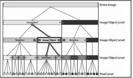
The pixel based method is very useful for the image classification but the LULC categories can be represented better by objects rather than pixels, so the second step of the classification is using the object oriented method for the classification. Object oriented classification is based on image objects which mean a set of similar pixels (figure 3-9). For acquiring these objects the segmentation is the most common method. “Image segmentation is the process of partitioning a digital image into multiple segments” (Shapiro & Stockman, 2001). The main aim in segmentation is dividing the image into more meaningful smaller pieces and then the merging these pixels according to different algorithms.
Figure 3-9: Object based Classification (Caetano, 2009)
Common segmentation methods are, thresholding, clustering, region-growing, split-and-merge, watershed transformation, model based segmentation, trainable segmentation (Image Segmentation, n.d.). For this research watershed delineation and & similarity threshold based segmentation methods have been used for classifying the images.
3.2.1 Watershed Delineation Segmentation
The watershed delineation algorithm is using the pixel values within the variance, like elevation values in digital elevation model, then grouping the pixels in the same watershed catchment areas and giving the unique ID to this catchment area and then grouping/merging the pixels which have same watershed ID (Eastman, 2009). The segmentation process is iterative in this method every segment merged with the most similar group, for this purpose user defined similarity threshold, weight variance and weight mean vector were used. For the study threshold value was 5, because the study area composed of mixed pixels for this reason the similarity threshold determined low for having smaller segments which includes fewer amounts of pixels but more similar (Eastman, 2012). After segmentation pixel based classification was used to as a reference image to have the final result. The result of the segmentation based images can be observed from figures 3-10, 3-11 and 3-12.
18
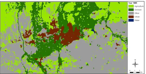
Figure 3-10: Segmentation based classification result (1990)
Figure 3-11: Segmentation based classification result (2000)
19
3.3 Accuracy Assessment
The last part of the image classification process is accuracy assessment. Accuracy assessment is a process to compare the classification with ground truth or reliable sources (Rossiter, 2004). For the accuracy assessment overall kappa which is a statistical measure of overall agreement between two categorical items (Cohen’s kappa, n.d.) and conditional kappa which includes, user’s accuracy, producer’s accuracy and overall accuracy were calculated. The mathematical explanation of the calculation process and the detailed results of the accuracy assessment can be found in appendix A. For this process we need ground truth data for testing sites, since this is not available the CORINE, STATIP and user interpretation has been used for selecting the testing sites. For each LULC class 19-50 random points were created and then the spatial information for these points acquired from CORINE and STATIP and compared with the satellite images. For the year 2010 the CORINE was not available because of that 2006 CORINE and Google Earth were used for creating the testing points. For each class the general requirement is 50 points (Lillesand & Kiefer, 2004), since the water bodies don’t cover a huge area only 19 points were created for water bodies in each LULC time. The method used for accuracy assessment is a comparison technique which is comparing the testing points with the classified image for the each land cover class. Accuracy assessment results for the segmentation based images:
1990: Overall Kappa : 0.7685
2000: Overall Kappa : 0.7256
2010: Overall Kappa : 0.7511
This level of accuracy found as satisfactory because of the heterogeneity of the study area and the low resolution of the satellite images and according to kappa agreement the accuracy was in substantial agreement level which means it can be used (Pontius, 2000).
< 0: Less than chance agreement
0.01–0.20: Slight agreement
0.21– 0.40: Fair agreement
0.41–0.60: Moderate agreement
0.61–0.80: Substantial agreement
20
4 SUITABILITY ANALYSIS
Suitability analysis has importance on LULC change modeling process, because with the help of suitability analysis simulation for the future can be grounded with the existing patterns and drivers. The definition of the suitability in general is “quality of having the properties that are right for a specific purpose”, and for the land-use suitability we can specify the definition suitability as identifying the most appropriate spatial pattern of future land uses according to purpose (Hopkins, 1977). Suitability analysis can be used for different purposes such as, agriculture, ecology and urban development. According to each approach the objectives would be different. The criteria for urban suitability would be different than agricultural suitability because in each case the suitable places have different features (Malczewski, 2004). The features of each category need a different specialization, for instance; the suitable lands for agricultural development are different than the urban development. For this research the focus was the urban area expansion and impacts on other categories, because of that the suitability analysis has been done only for urban category.
Many studies have been done in order to find the urban suitability although the methods and variables dependent on location and time. Each location has its own patterns which have different effects on urban development; this can be depending on the rules and existing trends. For instance the past and present urban development trends are different; in the past the settlements were mainly built near to the industrial zones in order to decrease the travel time, but currently the developments no longer take place near the industrial zones on the contrary the industrial zones are tried to be decentralized. Moreover the urban development patterns are different in developing and developed countries. Therefore for this research the rules in Turkey and patterns in study area taken into consideration for the suitability analysis.
4.1 Multi Criteria Evaluation
For suitability analysis Multi Criteria Evaluation (MCE) is a widely used process. Finding the suitable areas for the urban development requires consideration of different drivers because of that using a system which evaluates multiple criterions are required. This process combines variables with different methodologies and then transforms it into a suitability map output (Drobne & Lisec, 2009). The main criterions in MCE are Factors, Constrains.
Constrains: Constrains are the variables which refer to the restricted areas for
development, there are no medium values; the values are either 0 (not suitable) or 1 (suitable) (Eastman, 2012).
Factors: Beside the constrains there are variables which effect the urbanization in a
continuous scale, different than the constraints they have medium values and this medium values have different suitability. So the factors can be defined as the variables which have continuous suitability values (Eastman, 2012).
21 The most common techniques in MCE are;
Boolean Intersection
Weighted Linear Combination (WLC)
Ordered Weighted Averaging (OWA) (Eastman, 2012)
4.1.1 Weighted Linear Combination
WLC is method is simply a weighted overlay operation of the different criterion. Beside the variables the main part of the process is the weight allocation of factors and using the factors and constraints in an overlay analysis in order to find the suitability of the area.
The formula of the Suitability according to WLC is:
S= Wi Xi) Ci
Where, S: suitability,
Wi: weight of factor i,
Xi: criterion score of factor i, Ci: criterion score of constraint j,
: Somme,
: Product (Eastman, 2012)
In this method continuous values (factors) were standardized to a numeric range and then combined according to the weights (Eastman, 2012) and then they were masked (product) by constrains to have the final suitability map. The standardization formula is:
X i = (R i -R min) / (R max -R min ) * standardized_range
R = raw score
Standardization of the factors can be done according to:
Fuzzy set membership approach,
Value/utility approach,
Function approach,
The probability approach
For this research fuzzy set membership approach used.
4.1.2 Fuzzy Set Membership
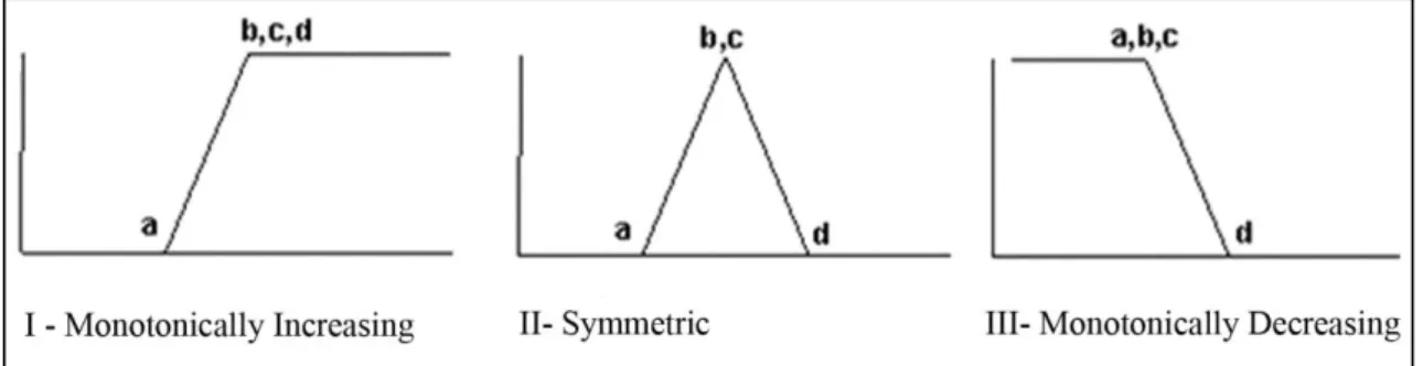
The fuzzy truth represents the membership in vaguely defined sets. This set doesn’t have sharp boundaries. For example distance terms like far-close are fuzzy truths because the definition of the proximity is not strict. In suitability analysis, especially if we deal with the proximity issue the fuzzy logic helps us to standardize the variables (Jiang & Eastman 2000). Some of the fuzzy set functions are Sigmoidal, J-shaped and Linear, and for this research linear function has been used (Eastman, 2009). There are different types of the linear function like presented in figure 4-1. These are illustrating
22
how the membership changes. For example in symmetric one the membership (suitability) increases from control point a to b and then decreases from c to d. (For detailed information about fuzzy logic the paper written by Jiang & Eastman (2000) can be referred).
Figure 4-1: Linear membership functions (Eastman, 2009)
4.1.3 Weight Decision
Weights are the values which indicate the impact of each criterion on the process. There are many methods to decide the weights of each factor, in general the weights can be determined by decision makers, but when there are many criterions the process become complex and using the Analytical Hierarchy Process would be a better solution for advanced works. In this system pairwise comparison method has been used, which indicates the relative importance of the each factor (Yu, Chen & Wu, 2009). In the table 4-1 it can be observed that in pairwise comparison table the scale is continuous and according to the importance there are extreme points.
Table 4-1: Continuous Rating Scale
1/9 1/7 1/5 1/3 1 3 5 7 9
extremely Very strongly
Strongly Moderately Equal Moderately Strongly Very strongly
extremely
Less important More Important
The pairwise comparison works like this: if one felt that accessibility is important than geological situation in determining suitability for urban development, one would enter a 5 on this scale. If the inverse (geological situation is more important) were the case one would enter 1/5.
4.1.4 Implementation of Suitability Analysis
In order to implement the suitability analysis first of all the variables in other words factors and constrains for the study area were defined.
23
4.1.4.1 Constrains
Constrains for this project are the locations which are not allowed for urban development by law or existing occupied areas like existing built up area where the development is not possible.
Archeological Lands: According to the regulations in Turkey urban development is
forbidden in the approved archeological zones (Protection and Utilization of Archeological Zones, 1999).
Protected Areas: Protected area category is mainly including the naturally protected
areas which are also not suitable for urban development (Rule for protection of Culturally and Naturally Important Areas, 1983).
Water Bodies: The urban development is not possible in water bodies.
Existing Built Up: These areas are already occupied so the further urban development
is not possible because the models are not considering the vertical growth (Ahmed, 2011). Vertical growth means the increase in the number of floors or replacement of the one storied houses with multiple storied houses which would increase density but not the area.
In figure 4-2 we can observe all constrains to be used in suitability process.
24
4.1.4.2 Factors
Factors for this research have been selected according to existing patterns and rules in Turkey. Factors are different than constrains because factors have continuous suitability values different than 0 and 1. The factors used for the study were in different scale so that they need to be standardized to the same scale in order to use in the suitability process. For the standardization of the factors fuzzy logic has been used because the suitability values of factors doesn’t have strict values which means fuzzy logic can be helpful. Moreover the factors also were in different level of measurement; some of them were nominal some were numeric. For the nominal factors the reclassification method used and for the numeric ones linear fuzzy set membership used.
Agricultural Lands: The agricultural lands are important for this research as a factor
because there are some rules and regulations available for protecting them. However we cannot take them as constrain because even though there are limitations, these areas have been transformed to urban areas. For the agricultural lands Ministry of Agriculture defined different classes, but for this research four of them used and their suitability scale decided according to regulations and then they were standardized to the scale 0-255. Agriculture variable was in nominal scale and this need to be transformed to 0-255 continuous scale. For this factor reclassification method has been used to standardize the values to 0-255 scale. For the class I and II; 0 and for class III; 80-120 and for class IV; 120-150 suitability values assigned and for the other areas 255 values assigned. This values are not strict we just try to show the level of suitability in a continuous scale.
Slope: Slope is an important factor in urban development because it affects the cost of
construction. Jantz, Goetz & Shelley (2004) stated that the effect of slope can change probability of urbanization in a specific location. Slope was in continuous scale but not in 0-255 and this need to be standardized. For this variable fuzzy set membership linear function used to standardize the slope values to 0-255 scale. Monotonically decreasing linear function used (Control points c=0, d=20). Which means between the 0-20 the suitability is decreasing and after 20 the suitability is 0 (LaGro, 2001).
Distance from Build Up: Urban development generally takes place near to existing
developments because of the existing infrastructure so the proximity to the existing built-up areas has higher suitability compared to the far areas (Araya & Cabral, 2010) (Ahmed & Ahmed, 2012). As it can be observed from the figure 4-3 the expansion of the urban area was mainly covering the previous boundary and it is located mainly in the periphery of the existing built up.
25
Figure 4-3: Urban area boundary changes
Proximity is fuzzy criterion because there aren’t exact boundaries to define the suitability, so we can just say proximity to existing built up increase the suitability. Distance from existing urban area was in continuous scale but not in 0-255 so this standardized by the monotonically decreasing linear function (Control points c=0, d=10000).Which indicated the suitability value decreases when we go far from urban area and after 10 km it is close to 0.
Distance from Main Roads: In developing countries urban development takes place
along the road (Kumar & Shaikh, 2012). As it can be observed from the figure 4-4 expansion of the urban area were mainly located along the main roads.
26
Moreover as it can be observed from figure 4-5 after 15 km the urban area is decreasing. According to this analysis we can say there is a strong relation between the roads and urban sprawl.
Figure 4-5: Trend chart for road & urban relation
In order to create the suitability related to proximity to road the fuzzy set membership symmetric linear function used. Because within 25m distance the area is not suitable urban development since it is including the road. In this case the control points were a=0 b=25 c=25 d=15000 this values means between the 0-25m the land is not suitable for urban growth, between the 25m to 15000m the suitability is degreasing near 25m it have the highest value after that it is decreasing in a continuous scale and after 15 km it is close to 0.
Geology (Earthquake risk): Geological conditions in other words earthquake risk
have an important influence on the urban development, especially after the destructive earthquakes take place in some cities in Turkey these conditions started to be taken into account. Tudes& Yigiter, (2010) used it for the suitability analysis of Adana city in Turkey, and they stated that the earthquake risk could change the suitability of the location; development should take place where there is low risk of earthquake. The earthquake risk map was in nominal scale it had three categories for the study area which are; Suitable area under control 1 (S1), Suitable area under control 2 (S2) and not suitable (NS) area. We order them according to their suitability. These values were in nominal scale in order to convert them to the 0-255 scale reclassification method used and according to the values the suitability degree in 0-255 scale arranged. S1 (230-255) > S2 (160-175)> NS (0). For this factor also we cannot say these values are strict, they have been selected in order to illustrate the level of suitability.
Previous Plans: Previous plans also selected as a factor because in Turkey if there will
be a new development this areas are the first places to consider for the expansion so they are more suitable than the other areas. This factor was in nominal level to so this transformed to 0-255 scale by reclassification method. The new development areas categorized as 255 (high suitability) and the other areas in the periphery indicated as 0 (low suitability).
27
In the figure 4-6 we can observe the standardized suitability maps of each factor defined. From the legend we can observe the pink color represent the highest suitability which is 255 and the black indicates the lowest suitability value which is 0.
Figure 4-6 : Standardized factors
After defining the factors and constrains and then standardize them the next step is to define the weights of the factors. In order to decide the importance of each factor urban planning expert’s opinions were used. According to their opinions the relative importance of the factors determined and the pairwise comparison matrix generated. (Questionnaire form filled by experts can be founded in appendix C).
28
Table 4-2 : Pairwise comparison matrix
According to this pairwse comparison table 4-2 the weights were calculated.The weight of the each facto can be observed from table 4-3.
Table 4-3: Weight of Factors
Class Weight
Agricultural Lands 0.0502
Geology 0.4072
Accesibility (Distance to Roads) 0.1244
Slope 0.1701
Distance to Existing Urban Areas 0.1149 Previous Plan Boundaries 0.1332 *Consistency ratio (CR)= 0.04 is acceptable
* A measure of how far a matrix is from consistency is performed by Consistency Ratio (CR) (Kordi, 2008). If CR > 0.10, then some pairwise values needs to be reconsidered and the process is repeated till the desired value of CR < 0.10 is reached
Factors Agricultural Lands Geology Accesibility (Proximity to Roads) Slope Proximity to Existing Urban Areas Previous Plan Boundaries Agricultural Lands 1 Geology 5 Accesibility (Distance to Roads) 3 1/5 Slope 3 1/3 1 Proximity to Existing Urban Areas 3 1/3 1 1 Previous Plan Boundaries 3 1/3 1 1/3 1 1
29
4.2 Suitability Analysis Results
Figure 4-7: Urban suitability
In figure 4-7 we can observe the results of the suitability, here the white color indicates the high suitability and the black indicates the low suitability. In the map as we can observe that constrains was illustrated as black because in these areas urban expansion was not possible.
This suitability map will be used in modeling process in order to ground the model with existing patterns and expert opinions. This might help us to increase the accuracy of the model for the urban class by training the model with existing pattern and expert
30
5 CHANGE DETECTION ANALYSIS
Change detection is the process of identifying differences in the state of an object or phenomenon by observing it at different times (Singh, 1989). The land change can be resulted by many factors, in order investigate these factors we need to analyze the changes. By change detection method transitions from one category to other ones can be observed, which can help to understand the interaction between the categories. There are many techniques for change detection. For this research cross tabulation, area calculation, reclassification and the overlay methods were used. Cross tabulation is a statistical process that shows the joint distribution of two or more variables (Cross Tabulation, n.d.). Reclassification is simply classifying the one image according to new categories. Overlay simply means combining information from different layers. By using these methods amount of gain and losses, net change, and contributor to change from each category were calculated (Johnson, 2009). With this method the changes in each category have been observed. As it can be observed from the figure 5-1 in each class there are some gains and loses. Some of them are real changes in the study area and some of them are inaccurate changes resulted from the misclassification of the satellite images.
5.1 Changes between 1990-2000
The figure 5-1 prepared in order to investigate the gains and losses from each category. As we can observe from the figure there are big losses in each class especially in agriculture class and orchard.
31
In order to observe the transformation from agriculture and orchard to urban area the figure 5-2 and table 5-1 prepared. The locational contribution to urban area from other classes can be observed from figure 5-2 and the areal changes summarized on the table 5-1. As we can observe from table 5-1 around 900ha of these categories was transformed to urban area.
Figure 5-2: Transition from other categories to urban (1990-2000)
Table 5-1: Transition from other categories to urban (1990-2000)
In this study one of the important objectives was to observe the changes in orchard in order to observe the changes in this category in detail the figure 5-3 prepared, as we can observe the main losses from this category was to urban and the gains were mainly from agriculture and other class.
Transition Area (ha)
Agriculture to Urban 384.31
Other to Urban 575.84
32
Figure 5-3 : Contribution from other categories to orchard (1990-2000)
From figure 5-4 it can be observed that there was a decrease in agricultural lands due transformation to urban class and other class. The transformation from agriculture to other class might be caused by changes in fertility of the land or resulted from misclasification. In image clasification phase it has been founded that the agriculture class and other usages has a similar reflectance values in some areas, this could mislead the process, because of that here we will mainly concentrate on transformation to urban class.
Figure 5-4 : Contribution from other categories to agriculture (1990-2000)
5.2 Changes between 2000 -2010
After observing the changes in the year 1990-2000, the changes in 2000-2010 also investigated in order to understand the change trend in the study area. As it can be observed from figure 5-5 in each class there are some gains and losses. The main transformations are from orchard and agriculture to urban area again.
33
In order to understand the locational distribution of the transition to urban area illustrated in figure 5-6 and table 5-2 in order to observe the transformations according to location and quantity.
Figure 5-6: Transition from other categories to urban (2000-2010)
As we can observe from figure 5-6 and table 5-2 the urban area increased more than 1500 ha and this mainly observed in outskirts.
Table 5-2: Transition from other categories to urban (2000-2010)
Transition Area (ha)
Agriculture to Urban 596.12 Other to Urban 614.25 Orchard to Urban 471.55
Furthermore the changes in orchard and agriculture has been observed for this period. As we can see from the figure 5-7 the decrease in orchards mainly resulted from urban area increase.
34
Figure 5-7: Contribution from other categories to orchard (2000-2010)
Moreover the agricultural changes mainly were resulted by other class and urban area increase. As it has been mentioned the transformation from agriculture to other might be resulted because of misclassification so that these changes ignored. As we can observe from the figure 5-8 there is a huge transformation between other class to agriculture which can be a result of misclassification of the classes in different years.