Optimal experimental design for estimating the kinetic parameters of processes described by the Weibull probability distribution function

Optimal Experimental Design for Estimating the Kinetic

Parameters of Processes Described by the Weibull

Probability Distribution Function

Luis M. Cunha”, Fernanda A. R. Oliveira”* & Jorge C. Oliveira”

“Es&a Superior de Biotecnologia, Universidade Catolica Portuguesa, Rua Dr. Antonio Bernardino de Ahneida, 4200 Porto, Portugal

“Instituto Inter-Universitario de Macau, Palacio da Penha, Macau, Portugal (Received 1 December 1997; accepted 26 May 1998)

ABSTRACT

The optimum experimental design for determining the kinetic parameters of the model resulting from the Weibull probability density junction was studied, by defining the sampling conditions that lead to a minimum confidence region of the estimates, for a number of observations equal to the number of parameters. It was found that for one single isothermal experiment the optimum sampling times corresponded always to fractional concentrations that are irrational numbers (approximately 0.70 and 0.19) whose product is exactly l/e’. The experimental determination of the equilibtium conversion (for growth kinetics) is vety important, but in some situations this is not possible, e.g. due to product degradation over the length of time required. Sampling times leading to a maximum precision were determined as a function of the maximum conversion

(or yield) attainable. For studies of kinetic parameters over a range of temperatures, performed with a minimum of three isothermal experiments, it was proved that the optimum design consists of two experiments at one limit temperature with two sampling times (those corresponding to fractional concentrations of approximate[v 0.70 and 0.19) and another at the other limit temperature for a sampling time such that the fractional concentration is lie. Case studies are included for clarijication of the concepts and procedures.

NOMENCLATURE

c; Number or concentration of a component or quality factor at time t, Ci,,, Initial concentration of a component or quality factor

C, Equilibrium concentration of a component or quality factor

Ea Activation energy (kJ mol.- ‘)

*Author to whom correspondence should be addressed. 175

176 E.D. LID F n P R T ti Uf

Efficiency of the design (%)

Ratio between bed length and diameter

Matrix of the derivatives of the response function Number of experimental points

Number of parameters

Universal gas constant (kJ mol-’ K-‘) Temperature (“C)

Sampling time of experiment i (min) Superficial velocity (m/s) Greek letters a r A max At re’

Scale parameter (min)

Pre-exponential scale parameter (min) Shape parameter

Modulus of the determinant of F (min-’ or min-’ ‘C-l)

Modulus of the determinant of F for optimal conditions (min-’ or min-’ ‘C-l)

Time lag between tl and tz (min)

Fractional concentration for the experiment i Vector of p parameters

his A4. Cunha et al.

INTRODUCTION

The Weibull distribution is one of many probability distribution functions used to describe the behaviour of systems or events that have some degree of variability. It was originally developed in 1939 by W. Weibull to statistically analyse the ultimate strengths of materials (Simon & Woeste, 1980). The probability density function of the Weibull distribution may be described as (Hahn & Shapiro, 1967):

(1)

0, elsewhere

with c( > 0 and fi > 0. The corresponding cumulative distribution is:

F(t)= s

’

f(t)dt= 1 -e-(t)” ₍₂₎

0

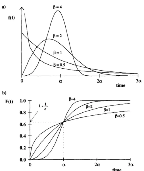
This model has an interesting potential for describing microbial, enzymatic and chemical degradation kinetics (failure of the system after a given time subjected to stress conditions), considering the scale parameter (u) as a reaction rate constant and the shape parameter (8) as a behaviour index. The model reduces to a first order decay/growth kinetics for p = 1 (see Fig. 1). As discussed by Hahn and Shapiro (1967) Nelson (1969) and Gacula and Kubala (1975), the failure rate for the Weibull model is an increasing function of time for fl> 1 and a decreasing function for p < 1. When /I = 1, the failure rate is constant. These authors also

Optimal design of experiments for the Weibull model 177

emphasise that cc is a characteristic time to failure, as it corresponds to the lOO*(l -l/e) = 63.2 percentile of the distribution, regardless of the value of /3 (see Fig. l(b)).

The Weibull distribution was successfully applied to describe shelf-life failure (Gacula & Kubala, 1975; Schmidt & Bouma, 1992). Page (1949) developed an equation to describe thin-layer drying of shelled corn, similar to the Weibull proba-

b)

F(t)

1.0

Fig. 1. Effect of the shape parameter /I on (a) the Weibull probability density function, f(t), (b) the Weibull distribution function, F(t).

178 Luis M. Cunha et al.

bilistic model that was later used to model thin-layer drying of yellow corn (Misra & Brooker, 1980; Li & Morey, 1984), of soybeans (White et al., 1981) of pigeon pea (Shepherd & Bhardwaj, 1988) and of adzuki beans (Tagawa et al., 1996). This model was also used to describe the drying kinetics of rough rice (Agrawal & Singh, 1977; Wang & Singh, 1978; Lu et al., 1994). Chhinnan (1984) evaluated four mathematical models, i.e., the exponential model, the diffusion model, an approximation of the diffusion model and the Page (Weibull) model, for describing thin-layer drying of in-shell pecans, recommending the Page (Weibull) equation for future modelling studies. Moreover, the Weibull distribution has been used to model failure of apple tissue under cyclic loading (McLaughlin & Pitt, 1984) grape pomace elutriation (Peraza et al., 1986) and water uptake and soluble solids losses during rehydration of dried apple pieces (Ilincanu et al., 1995). Machado et al. (1997) adequately

described moisture uptake and soluble solid losses by breakfast cereals immersed in water or milk using the Weibull model, after unsuccessful attempts to use the Peleg (1988) the diffusion and the first order models. Recently, the Weibull model has also been used to describe microbial death kinetics under high-pressure conditions (Heinz & Knorr, 1996).

As in any other model, the usefulness of the Weibull model for predictive or descriptive purposes greatly depends on the precision and accuracy of the model parameter estimates. Rigorous parameter estimation requires an adequate statistical analysis of experimental data, but also a careful experimental design. As stressed by Bates and Watts (1988), even very careful data analysis is unable to recover infor- mation that is not present in the experimental data.

Box and Lucas (1959) proposed an optimum design criterion for non-linear models that allows the selection of sampling conditions that lead to a minimum confidence region, also known as D-optimal design (Bates & Watts, 1988). The rationale is that as the ‘real’ parameters of a system are probably contained in the error region of the estimates, the smaller this region the higher the precision. This criterion has been applied in different situations, such as, first order kinetics under isothermal conditions (Box & Lucas, 1959) diffusional processes under non-iso- thermal conditions (Oliveira et al., 1995) and the Thermal Death Time model under both isothermal and non-isothermal conditions (Cunha et al., 1997).

The main objective of this work was to define the best experimental conditions according to the D-optimal design for systems that may be described by the Weibull probabilistic model.

MATHEMATICAL METHODS

For any choice of the design variable (i.e., the independent variable, t) the size of the parameters joint confidence region is proportional to the Jacobian 1 (FTF) 1 p1’2 of the derivative matrix F (where Fr [j&l, with fi,l = axiKNj evaluated at t = ti with i ranging from 1 to n; x represents the system response and 8 is a kinetic parameter). Thus, a logical choice of the design criterion is to choose sampling points so that the size of this joint confidence region is minimised, that is, the determinant D = 1 FTF 1

should be maximised. This can be done for a number of sampling times equal to the number of parameters to be estimated, which is the minimum possible. Atkinson and Hunter (1968) showed that for a number of observations greater than the number of parameters, the optimal design often corresponds to r replications of the

Optimal design of experiments for the Weibull model 179

optimal p sampling times (r = n/p). According to Box and Lucas (1959) if a sequence of n observations is to be designed for a p-parameter model, in the case where n =p, the D-optimal design can be simplified from the maximisation of D z lFTF 1 to the maximisation of A = mod( IFI ) (A denotes the modulus of the determinant of the matrix F). Due to the complexity of the mathematical expres- sions of A derived for the Weibull model, there was no analytical solution, and therefore a numerical procedure was used. Numerical optimisation was performed using Mathematics@ for Windows-2.2 Enhanced Version (Wolfram, 1993).

If one considers that: (i) vi corresponds to (Ci -C,)l(Ci,i -C,), the fractional amount of a given component C, changing from an initial value (Cini) to a final equilibrium value (C,), at a time t, and that (ii) the time required to reach a certain value of q is represented by the continuous random variable z, with probability density function f(t), where f(t) is the Weibull distribution function, then q(t) can be defined as the probability of having a certain fractional amount of C for, at least, a specified time t, under specified experimental conditions. Therefore:

q(t) = P(z > t) = s

,: f(r)dr = 1 -F(t)

Experiments conducted at a single temperature

(3)

Combining eqns (2) and (3) the response function estimated at time t,, can be expressed as:

Cj=C, +(Ci”i-C,)rli=C,+(Ci,i-C,,)e~ _i $ ₁ ” ₍₄₎ Following the procedure presented by Box and Lucas (19.59) the determinant, A, of the matrix of derivatives of the response function in order to the model parameters, was built for four time levels tO, tl, t2 and tj. For the sake of simplification, A is represented in terms of q: / A=mod \

ace ace

--

act

ag

ac, ac,

-

-

ag

ac2

-

-

aa ag

ac3

--

a@ ag

ac, ac,

--

acx

ac,

ac,

-

-

ac,x

ac,, ac2

-

-

ac,

ac,

-

-

ac,

ln(rloh2

180 Luis A4. Cunha et al. xIn w/2) [

1

Wd

-

h -

[ I

-

1

Mr/3)

[ 1

(5)

As stressed by Cunha et al. (1997), when the initial concentration, Cini, is considered to be a model parameter one of the optimal sampling times would be equal to zero (the time at which the initial concentration is determined), leading to q. = 1. Thus:

Similarly, when the equilibrium value is considered to be a model parameter, an optimal sampling time near infinity would be obtained, that is, y/3 = 0. Combining both results, the determinant A may be simplified as follows:

A=mod

Ccini

- cco)’ In

(q2)

CI

[ I)

I

₍₇₎

The optimal experimental design leading to a minimum confidence region was found by determining numerically the conversion values ql and y12 that maximise the modulus of A. Substituting these values back into eqn (4), the optimal sampling times, t, and t2, were obtained.

There are some practical cases where it is impossible or unfeasible to reach the equilibrium value because the time required might be too long and/or the food may degrade. In these cases sub-optimal designs should be developed, taking into con- sideration the maximum measurable value of ‘C3’, that is, the minimum value of ‘Y/~‘. Having this in mind, the determinant A of the matrix of derivatives of the response function in order to the model parameters was built for three time levels tl, t2 and t3. For the sake of simplification, A was again represented in terms of a system response v], the fraction by which the yield ‘c’ falls short of its equilibrium value.

Therefore, the values of Q and q2 that maximise the determinant in eqn (6) were also numerically obtained for different fixed values of q3, thus obtaining sub-optimal designs.

To have a better insight into the loss of precision in the parameter estimates due to the deviation of q3 from its optimum value (zero: Ci = C,), relative design efficiencies (E.D.) were computed for each value of q3, as defined by Neter et al.

(1966):

E.D.i = I(FTF)-‘I,i” “” I(FTF>- 'Ii

Optimal design of experiments for the Weibull model 181

Set of isothermal experiments conducted over a range of temperatures

As a rate parameter, c1 is temperature sensitive and l/a can be expected to follow an Arrhenius-type behaviour, as often found (Shepherd & Bhardwaj, 1988; Ilincanu et

al., 1995; Machado et al., 1997):

1

l

[-cl]

-z--e

cli a0

(9

The p parameter should indicate the kinetic pattern and thus be temperature independent, particularly within a limited range of temperatures. This result has been verified in published works (Chhinnan, 1984; Ilincanu et al., 1995; Machado et al., 1997). Therefore, the kinetic parameters of the model for practical situations in food processing are ao, Ea and p, as non-isothermal conditions are the most usual. These parameters can however be determined by performing isothermal experi- ments at different temperatures covering the range of interest. For this case, the model is:

In this situation, optimal designs require not only the selection of sampling times but also the selection of the temperatures that lead to a higher precision of the estimates. If isothermal experiments are performed, then one should select the most appropriate temperatures for the experiments and, for each temperature, the ade- quate sampling times. Non-isothermal experiments require the definition of both the temperature history and the sampling times but this case will not be analysed in this work.

The sampling times for Cini and C,, in case they are taken as model parameters, were already approached (t = 0 and t-co, respectively). It is eventually necessary to analyse whether C, is temperature independent or not. The subsequent analysis refers only to the determination of the three kinetic parameters and therefore Cini and C, are taken as known constants in the mathematical handling. Following the previous procedure, the determinant, A, of the matrix of derivatives of the response function in order to the model parameters, cxo, Ea and p, was determined for three time levels tl, t2 and t3 and three temperature levels T,, T2 and T3, respectively, yielding:

A=mod P(cini-Ca)3’11 lnhh lnh)q3 ln(q3) Q,RT, TZTJ

x [TIT* ln(z)+TJ, h($$-)+T,T, In(E)]) (11) The optimal experimental design leading to a minimum confidence region for any combination of temperatures (T,, T2 and T3) was found by determining numerically the conversion values ql, q2 and q3 that maximise the modulus of A. Substituting these values back into eqn (lo), the corresponding optimal sampling times: tl, t2 and t3, were obtained.

182 Luis A4. Cunha et al. RESULTS Experiments conducted at a single temperature

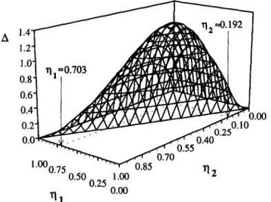
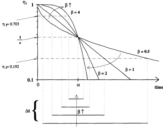
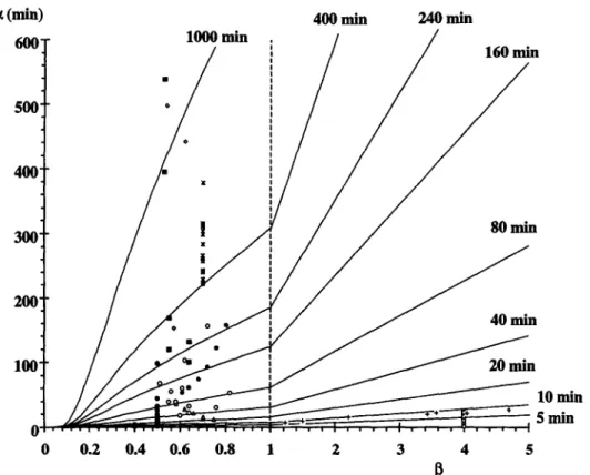
As discussed in the ‘Mathematical methods’ section, the complexity of eqn (7) prevented an analytical solution and the optimal design for the Weibull probabilistic model was numerically computed for a large number of different sets of the model parameters c( (between 0.1 and 600 min) and j3 (between 0.1 and 5). It was found that the fractional concentrations at the sampling times that maximised A were independent of the model parameters. In all cases, the solution of the optimisation problem was a pair of irrational numbers, identical to those obtained by Cunha et al. (1998) for the optimal experimental design for systems following the Thermal Death Time model under nonisothermal conditions: y1 = 0.70322.. . and q2 = 0.19245.. . , which are such that their product is equal to l/e2. Figure 2 shows how the determi- nant A from eqn (7) typically evolves as a function of the fractional concentration values, with its maximum occurring at the referred values of ql and q2. The two sampling points are symmetrical in a logarithmic scale in relation to l/e (see Fig. 3), this point corresponding to the optimal sampling point obtained by Box and Lucas (1959) for the simple exponential model (equal to the Weibull model for p equal to 1). It was further verified that if /3 is a known constant and c1 is the only parameter to be estimated, the optimal sampling time would also correspond to v] = l/e, inde- pendently of the value of p. It is noteworthy that the time lag between the two optimal sampling times decreases as the value of the shape parameter /I increases (see Fig. 3). Figure 4 shows the time lag between the optimal sampling times of the Weibull probabilistic model as a function of the model parameters CI and p. Each curve drawn indicates all pairs of c( and /3 that have the same time lag. Published

.oo

Fig. 2. Surface plot of A as a function of q1 and Q (eqn (7)). Maximum value of A is attained for v1 ~0.703 and q2 ~0.192.

Optimal design of experiments for the Weibull model 183

values of LX and p are also included. In general, the kinetics reported on literature show a value of jl lower than 1 and a value of LY such that the time lag is, in most cases, larger than 20 min. However, for Heinz and Knorr (1996) data and for some of the data from Machado et al. (1997), the p is so high and/or c( is so small, that this period either becomes unpractical or may lead to a considerable experimental error in the independent variable, t, that is not accounted for in the present analysis (see Fig. 4). A case study will be presented in the next section to illustrate how to handle this problem.

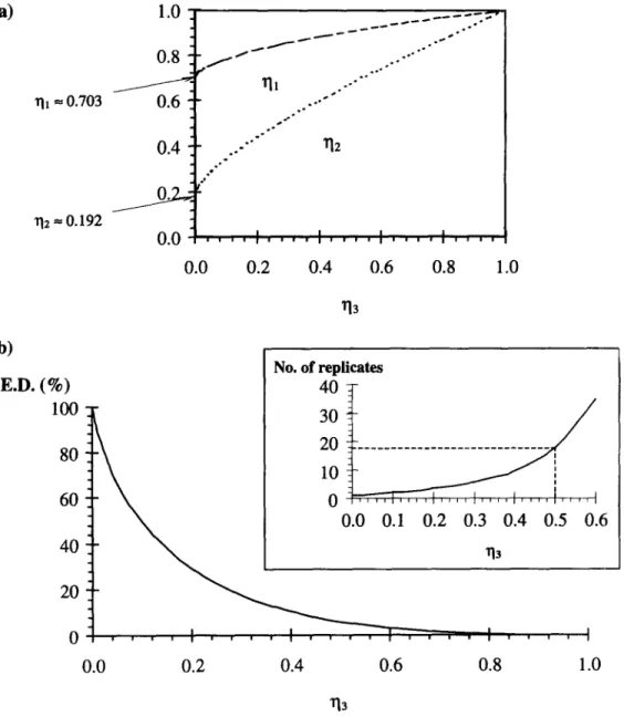
In growth kinetics, the equilibrium value (C,) is a very important parameter and should be evaluated at a sampling time near infinity, that is, at q = 0. However, sometimes the maximum attainable value of C is smaller than C,. In these situa- tions q3 is fixed by practical constraints and new optimal ql and y/2 values need to be calculated. It was found that as q3 increases, the optimal values of ql and q2 also increase and get closer (see Fig. 5(a)). The design efficiency (as computed from eqn (8)) strongly decreases when y13 increases (see Fig. 5(b)). It is also possible to translate this loss of efficiency in terms of the number of experimental data required to have the same precision of the estimates (i.e., same A). It is noteworthy that if,

1/----‘---- - ” ‘8, ” ‘<, ” ;.--_--~- llzco.192 0.1 : : : (--: :,:,:: : / time

Fig. 3. Identification of the optimal sampling points for the Weibull probabilistic model, evaluated at different values of the shape parameter fl.

184 Luii M. Cunha et al.

for example, one can only follow up a certain process until 50% of the total conversion (q3 = O-5), design efficiency will drop so strongly that in order to have the same precision the number of sampling points required would be approximately 18 times larger, when compared to the full optimal design (see small graph in Fig. 5(b)). Thus, even for relatively low values of q3, the application of optimal designs may not be enough to prevent significant loss of precision in the estimation of the model parameters.

Set of isothermal experiments conducted over a range of temperatures

The results of Box and Lucas (1959) for the first-order reaction model and those of

Cunha et al. (1997) for the isothermal Thermal Death Time model, showed that

when analysing a given system over a range of temperatures, an experiment should

400 min 240 min

0 0.2 0.4 0.6 0.8 1 2 3 4 5 B

Fig. 4. Time lag between the optimal sampling times of the Weibull probabilistic model as a function of the model parameters c( and /I. Each curve drawn indicates all pairs of c( and /I that have the same time lag (iso-time lag curves). Published values of CI and /I are indicated according to the following legend: *, Chhinnan (1984); q , Heinz and Knorr (1996); o, Ilincanu et al. (1995); A, Li and Morey (1984); l , Machado et al. (1997); o, Misra and Brooker (1980); +, Peraza et al. (1986); l , Shepherd and Bhardwaj (1988); and w, White

Optimal design of experiments for the Weibull model 185 be performed at each of the limit temperatures in order to obtain the maximum precision of the parameters of the model. Under those circumstances, sampling times corresponding to a conversion value equal to l/e, should be taken at each limit temperature. By analogy, and taking into consideration that the Weibull model

4

0.8

:-,R-~

.--

.-

..-

f

.:-

_.-*

0.0 = VII I‘S * I ; 1 ,,,I

,,,,f

0.0 0.2 0.4 0.6 0.8 1.0

b)

E.D.(%)

0.0

0.2 0.3 0.4 0.5 0.6

0.2

0.4

0.6

0.8

1.0

Fig. 5. D-optimal design for the Weibull probabilistic model when the maximum conversion value (11~) falls short of equilibrium (r/3 = 0): (a) optimal sampling values; (b) efficiency of the sub-optimal designs. The number of replicates required to have the same precision (small

186 Lui’s M. Cunha et al.

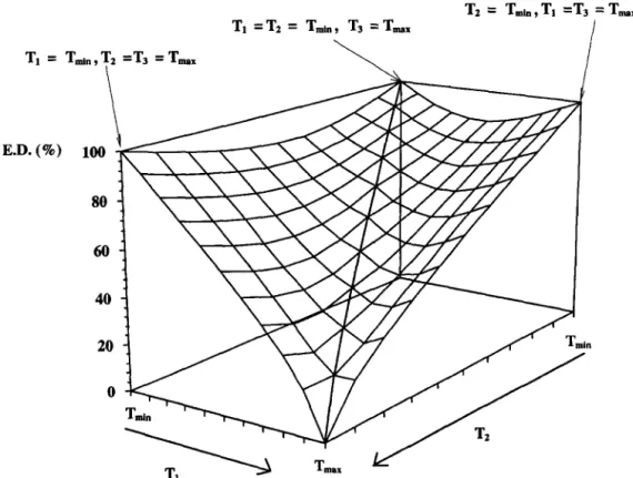
under these conditions has three parameters, it would be expected that there should be an experiment at each of the limit temperatures, with a third data point being taken at any given temperature between Tmin and T,,. In order to analyse this situation, A (from eqn (11)) was maximised considering T1 = Tmi”, T3 = T,,, and covering different values of T2, ranging from Tmin to T,,,. Furthermore, the effect of changing T1 from Tmin to T,,,, was also assessed. Figcure 6 shows how the design efficiency typically evolves with sampling temperature using T3 = T,,, and it can be clearly seen that the best design is T1 = T2 = Tmin with T3 = T,,,, T1 = Tmin with

T2 = T3 = T,,,, or T2 = Tmin with T1 = T3 = T,,,. Lower efficiency values were obtained whenever Tmin < T3 < T,,,, whatever the values of T1 and T2. Maximisation of A in order to ql, q2 and y3, for T1 = T2, yielded the following optimal design: yll = 0.70322.. ., yl?; = 0.19245.. . and q3 = l/e. Thus, when considering a range of temperatures, two sampling points should be taken at an extreme temperature, corresponding to fractional concentrations of O-70322.. . and O-19245.. . The remaining sample should be taken at the other extreme temperature at the time when the fractional concentration of l/e is expected.

T, = E.D. (%) Tz = T,,,,,,,T1 =T3 = TI =Tz = T,,,,,,, T3 =T,, _I T ml,,, T2 =4 = ‘La, _\ T mpx

Fig. 6. Efficiency of the D-optimal design for the Weibull probabilistic model with an Arrhenius temperature dependency of the scale parameter a, as a function of the sampling

Optimal design of experiments for the Weibull model 187

CASE STUDIES

To clarify the application of some of these concepts in food research, some case studies are presented using data from literature.

Separation of grape pomace in a fluidised bed

To model the simultaneous effect of drying and separation of grape pomace in a fluidised bed, Peraza et al. (1986) have used the Weibull model, as mentioned in the introduction. In this work, they have measured as a response function the grape skin fraction in the bed at any time (q) and modelled grape pomace elutriation as a function of fluidisation velocity (ur) and length/diameter ratio (L/D) of the fluidised bed. For the case where ur = 5.0 m/s and L/D = 4, the Weibull model yielded the following parameters: x = 26.275 min and p = 4.701. If one would intend to perform the same study using an optimal design, samples should be taken at t, ~21.0 min (time at which ~~0.703) and at t 2 ~29.2 min (time at which v] ~0*192), the time lag between ti and t2 (At) being therefore 8.2 min. From an experimental point of view, these sampling times are perfectly feasible. The heuristic experimental design used by Peraza et al. (1986) was based on six sampling points equally spaced in time, with a time lag of 5 min (t = 5, 10, 15, 20, 25 and 30 min); comparing this design with the corresponding optimal sampling procedure (three replicates taken at t = 21.0 min and three at t = 29.2 min), its efficiency (eqn (8)) would be approximately 52%. This means that the heuristic design used by Peraza et al. (1986) would require twice as many points as the optimum design to have roughly the same precision of the parameters estimated.

Soluble solids losses during rebydration

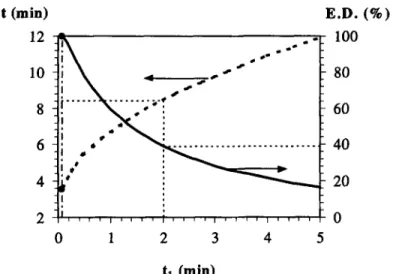
Considering a different situation, Machado et al. (1997) have modelled the soluble solid losses by puffed breakfast cereals immersed in water at 55°C where the Weibull model yielded the following parameters: c( = 1.04 min and /I = 0.4. To per- form the same study using an optimal design, according to those values, samples should be taken at t, ~0.08 min and at t2 - -3.62 min, with a resulting time lag of 3.54 min. While the time lag between sampling times appears to be experimentally manageable, the first sampling time may be unfeasible. If this requirement becomes an experimental hurdle, the optimal design cannot be applied. However, sub-opti- mal designs may be defined, for a pre-selected first sampling time (t,), if the determinant in eqn (7) is maximised as a function of t2 only (and thus as a function of the time lag between samples). Figure 7 shows the results obtained for values of t, up to 5 min, together with the respective design efficiency (eqn (8)). If: for example, one decides to establish a first sampling time equal to 2 min, the second sampling point should be taken at approximately 10.4 min (At z 8.4 min; see Fig. 7) with corresponding fractional concentration values of 0.27 and 0.08, respectively. The resulting efficiency would however be around 40% (see Fig. 7).

Microbial death kinetics under high pressure

Heinz and Knorr (1996) used the Weibull model to describe microbial death kinetics under high pressure conditions. Taking the example at a temperature of

188 Luis M. Cunhu et al. At (min) E.D. (%) 12 10 8 6 4 2 100 80 60 40 20 0 tl (min)

Fig. 7. Sub-optimal designs when fixing the values of tr, for Machado et al. (1997) parameters concerning the loss of soluble solids by puffed breakfast cereals immersed in water at 55°C. The plot gives the Ar (f2-fr) values for any tr in the left axis and the corresponding efficiencies of the design in the right axis. (0) Optimal sampling conditions: tr = 0.08 min;

Ar = 3.55 min and E.D. = 100%.

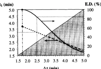
40°C and a pressure of 250 MPa the parameters reported were: a = 4.819 min and p = 4. To perform experiments using an optimal design, samples should be taken at ti ~3.71 min and at t2 ~5.46 min, with a resulting ti of 1.75 min. This time lag is relatively small and thus a larger lag may be preferred. Sub-optimal conditions were studied for this situation, constraining the value of the time lag and maximising the determinant in eqn (7) in order to one of the sampling times only, for values of b up to 5 min. Figure 8 shows the results obtained. If, for example, one decides to select a time lag of 2.5 min, the first sample should be taken at ~3.26 min (there- fore, t2 = 5.76 min), and the efficiency of this sub-optimal design would be around 85% (see Fig. 8).

For many experimental studies, the initial concentration (Cini) is not necessarily measured at t = 0, as the factor under study shows high stability over a given period of time. However, there are systems and/or variables for which Cini must be mea- sured exactIy at t = 0, as the factor will change over a short period of time. Under these circumstances, care should be taken when the minimum At is too high, as the first sampling time might be lower than L\t and t, is a time lag to zero. This is shown by the shaded part of the graph.

CONCLUSIONS

The optimal experimental design for determining the Weibull model parameters with the minimum possible error region for a number of points equal to the number of parameters at a constant temperature T consists of taking a sample at the time

Optimal design of experiments for the Weibull model 189 t1

bw

60

40

20

0

2.0 2.5 3.0 3.5 4.0 4.5 5.0

At(min)

Fig. 8. Sub-optimal designs when fixing time lag between the two sampling points, for Heinz and Knorr (1996) parameters concerning the death kinetics of Bacillus subtilis at 40°C and 250 MPa. The plot gives the t,-value for any At (t2 = t,+ At) in the left axis and the corre- sponding efficiencies of the design in the right axis. The shaded area indicates designs that may not be logical, as t, is lower than At. (0) Optimal sampling conditions: tl = 3.71 min;

At = 1.75 min and E.D. = 100%.

q2 = 0.19245.. . ) with qI*q2 = l/e2. Assuming that l/a follows an Arrhenius-type tem- perature dependency and /3 is independent of temperature, the optima1 experimental design to determine the system parameters for temperature dependent situations with isothermal experiments consists of two experiments, performed at the limit temperatures of the range of interest. In one, two samples should be taken, one when the conversion is uI = 0.70322.. . and another when q2 = O-19245.. . , while in the other experiment one sample should be taken where u3 = l/e.

The initial concentration and the equilibrium concentration (if different from zero) should be determined by analysing samples, respectively, at time zero and at a significantly large time so that q is constant (Ci-C,).

ACKNOWLEDGEMENTS

The authors acknowledge financial support from the EU projects AIRI-CT92- 0746 and STD3-CT94-0333. The first author acknowledges financial support from Fundacdo para a Ciencia e a Tecnologia (FCT) through ‘Sub-programa Ciencia e Tecnologia do 2” Quadro Comunitario de Apoio’. We also thank Andreia Pinheiro Torres for her helpful advice.

REFERENCES

Agrawal, Y. C. & Singh, R. P. (1977). Thin-layer drying studies on short-grain rough rice. ASAE Paper No. 77-3531, ASAE, St Joseph, MI.

190 Luis M. Cunha et al.

Atkinson, A. C. & Hunter, W. G. (1968). The design of experiments for parameter estima- tion. Technomettics, 10, 271-289.

Bates, D. M. & Watts, D. G. (1988). Nonlinear Regression Analysis and Its Applications, pp. 121-127. Wiley, New York.

Box, G. E. P. & Lucas, H. L. (1959). Design of experiments for non-linear situations.

Biomettika, 46, 77-90.

Chhinnan, M. S. (1984). Evaluation of selected mathematical models for describing thin-layer drying of in-shell pecans. Transactions of the ASAE, 27, 610-615.

Cunha, L. M., Oliveira, F. A. R, Brandao, T. R. S. & Oliveira, J. C. (1997). Optimal experimental design for estimating the kinetic parameters of the Bigelow Model. Journal of Food Engineeting, 33, 11 l-128.

Gacula, M. C. Jr & Kubala, J. J. (1975). Statistical models for shelf life failures. Journal of Food Science, 40, 404409.

Hahn, G. J. & Shapiro, S. S. (1967). Statistical Models in Engineering. Wiley, New York. Heinz, V. & Knorr, D. (1996). High pressure inactivation kinetics of Bacillus subtilis cells by

a three-state-model considering distributed resistance mechanisms. Food Biotechnology, 10,

149-161.

Ilincanu, L. A., Oliveira, F. A. R., Drumond, M. C., Machado, M. F. & Gekas, V. (1995). Modelling moisture uptake and soluble solids losses during rehydration of dried apple pieces. Proceedings of the Copernicus First Main Meeting-Process Optimisation and Minimal Processing of Foods, December 1995, ESB, Porto, Portugal.

Li, H. & Morey, R. V. (1984). Thin-layer drying of yellow dent corn. Transactions of the ASAE, 27,581-585.

Lu, R., Siebenmorgen, T. J. & Archer, T. R. (1994). Absorption of water in long-grain rough rice soaking. Journal of Food Process Engineeting, 17, 141- 154.

Machado, M. F., Oliveira, F. A. R. & Gekas, V. (1997). Modelling water uptake and soluble solids losses by puffed breakfast cereal immersed in water or milk, Proceedings of the Seventh International Congress on Engineering and Food, Brighton, UK.

McLaughlin, N. B. & Pitt, R. E. (1984). Failure characteristics of apple tissue under cyclic loading. Transactions of the ASAE, 27, 31 l-320.

Misra, M. K. & Brooker, D. B. (1980). Thin-layer drying and rewetting equations for shelled yellow corn. Transactions of the ASAE, 23, 12.54-1260.

Nelson, W. (1969). Hazard plotting for incomplete failure data. Journal of Quality Technology,

1, 27-52.

Neter, J., Kutner, M. H., Nachtsheim, C. J. & Wasserman, W. (1966). Applied Linear Statistical Models, 4th ed., pp. 128991293. Irwin, Chicago.

Oliveira, F. A. R., Silva, T. R. & Oliveira, J. C. (1995). Optimal experimental design for estimation of mass diffusion parameters using non-isothermal conditions. Proceedings of the First International Symposium on Mathematical Modelling and Simulation in Agriculture and Bio-Zndustries of IMACSIFAC, 9-12 May, Brussels, Belgium.

Page, G. E. (1949). Factors influencing the maximum rates of air drying shelled corn in thin layers. M.Sc. thesis, Purdue University, Lafayette, IN.

Peleg, M. (1988). An empirical model for the description of moisture sorption curves. Journal of Food Science, 53, 1216-1219.

Peraza, A. L., Pena, J. G., Segurajauregui, J. S. & Vizcarra, M. (1986). Dehydration and separation of grape pomace in a fluidized bed system. Journal of Food Science, 51, 206-210.

Schmidt, K. & Bouma, J. (1992). Estimating shelf-life of cottage cheese using hazard analysis.

Journal of Dairy Science, 75, 2922-2927.

Shepherd, H. & Bhardwaj, R. K. (1988). Thin layer drying of pigeon pea. Journal of Food

Science, 53, 1813-1817.

Simon, J. C. & Woeste, F. E. (1980). A system-independent numerical method to obtain maximum likelihood estimates of the three parameter Weibull distribution. Transactions of

Optimal design of experiments for the Weihull model 191

the ASAE, 23,955-958, 963.

Tagawa, A., Kitamura, Y. & Murata, S. (1996). Thin layer drying characteristics of adzuki beans. Transactions of the ASAE, 39,605-609.

Wang, C. Y. & Singh, R. P. (1978). A single layer drying equation for rough rice. ASAE Paper No. 78-3001. ASAE, St. Joseph, MI.

White, G. M., Bridges, T. C., Loewer, 0. J. & Ross, I. J. (1981). Thin-layer drying model for soybeans. Transactions of the ASAE, 24, 1643-1646.

Wolfram, S. (1993). Mathematics@. A System for Doing Mathematics by Computer, 2nd ed.. pp. 703-704, 794. Addison-Wesley Publishing Company, Reading, MA.