Computational simulation of a flow over the east part of the Madeira island

(1)

Computational simulation of a flow over the east

part of the Madeira island

João Pedro Leite da Silva

Dissertation:

Master’s in Mechanical Engineering

Supervisor: Prof. José Manuel Laginha Mestre da Palma

(2)

(3)

3 Dedicated to my mother and my father, who always gave their all to provide me the tools to get here and who always pushed me to be the best version of myself.

(4)

(5)

5

RESUMO

Este projeto centra-se no estudo de um fluxo de vento sobre uma região montanhosa no lado leste da ilha da Madeira. O objetivo principal consiste em rever o desempenho de um software genérico de CFD, ANSYS FLUENT, e como as suas configurações afetam o resultado final, ao mesmo tempo que se tenta recriar os resultados de [1].

Começou-se por realizar algumas simulações preliminares com malhas grosseiras onde se procurou uma familiarização com o software e as particularidades da simulação de fluxos de vento ao mesmo tempo que se definiu a altura do domínio de integração. Estudos mais detalhados seguiram, usando uma malha mais fina e modelos físicos mais precisos. Estes foram aplicados a simulações com ventos prevalentes de norte e de sul enquanto se experimentou com os métodos SIMPLE e coupled e as condições de fronteira de outflow e pressure outlet. Resultados mais rápidos e precisos foram obtidos com o método SIMPLE e a condição de fronteira outflow. Os resultados não foram totalmente validados pelo trabalho comparativo e alterações de terreno foram atribuídas como causas.

As características de fluxo foram analisadas com base em resultados numéricos de velocidades horizontais e longitudinais e também de quantidades de turbulência, como a intensidade de turbulência e a energia cinética de turbulência.

A disrupção do fluxo foi maior nas simulações com ventos prevalentes de norte, gerando campos de velocidade menos uniformes, maiores valores de quantidades de turbulência e mais zonas de estagnação e recirculação.

Finalmente, uma simulação transiente foi executada para detetar o comportamento com dependência temporal nas estruturas de vórtices originadas pelos ventos de norte.

(6)

(7)

7

ABSTRACT

This project focuses on the study of a wind flow over a mountainous region in the east side of the island of Madeira. The primary objective is to review the performance of a general purpose CFD software, ANSYS FLUENT, and how its configurations affect the final outcome, while trying to recreate the results of [1].

Firstly, preliminary simulations were performed with coarse meshes where one grew accustomed to the simulation software and to wind flow simulation particularities while also defining the integration domain height. More detailed studies followed, using a finer mesh and more accurately defined physical models. These were applied to northerly (north-prevailing) and southerly (south-prevailing) winds simulations while experimenting with the SIMPLE and coupled methods and the outflow and pressure outlet boundary conditions.

Faster and more accurate results were achieved with the SIMPLE method and the outflow boundary condition. The results were not fully validated by the comparative work and terrain changes were attributed as causes.

Flow characteristics were analysed based on numerical results of horizontal and longitudinal velocities and of turbulence quantities such as the turbulence intensity and the turbulence kinetic energy.

The disruption of the flow was bigger within the northerly simulations with less uniform velocity fields, bigger turbulence values and more stagnation and recirculation zones.

Finally, a transient simulation was run to detect time-dependent behaviour on vortices structures originated by northerly winds.

(8)

(9)

9

ACKNOWLEDGMENTS

I would like to express my gratitude to my supervisor, Prof. José Manuel Laginha Mestre da Palma, for his indispensable guidance and support throughout the course of this project. I am thankful for the support given by my colleague Carlos Silva who provided me with the elevation maps used.

Finally, I would also like to acknowledge all my friends of Tuna de Engenharia da Universidade do Porto, my second home during my academic journey, for their friendship, help and advices.

(10)

(11)

11

LIST OF TABLES

Table 1 - Default under-relaxation factors for the different variables in FLUENT. ... 29 Table 2 – Number of cell elements for each integration domain with a different height. ... 37 Table 3 – Spatial discretization methods for each variable used in the preliminary simulations. ... 39 Table 4 – Mesh metrics ratings according to a range of values. ... 45 Table 5 – Mesh metrics values obtained for the integration domains used in the northerly and southerly winds simulations. ... 46 Table 6 – Performance statistics for northerly simulations with different configurations. ... 50 Table 7 – Location of the five points of interest and RIX index. ... 98

(14)

(15)

15

LIST OF FIGURES

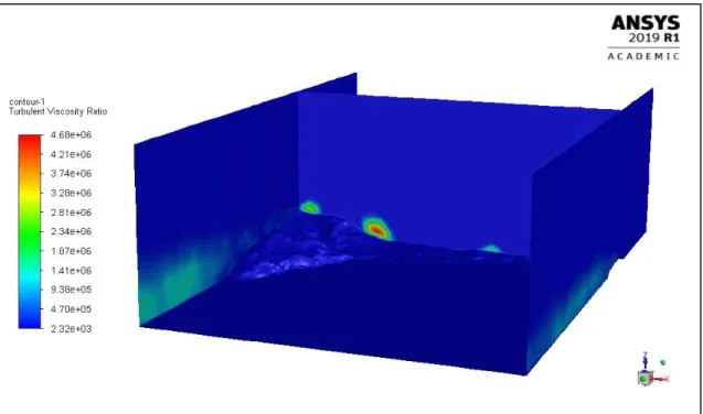
Figure 1 – Three-dimensional view of the modelled geographical area of study in the east region of the island of Madeira (north aligned with the positive direction of the y-axis). ... 22 Figure 2 - General view of the Workbench environment with an open FLUENT project. ... 23 Figure 3 – Step by step operations of a pressure-based segregated and a pressure-based coupled algorithm. ... 28 Figure 4 – Description of Compute normals for point sets and Screened Poisson Surface Reconstruction filters and parameters applied. ... 33 Figure 5 – Aspect of the geometry .stl file when imported into SpaceClaim (north aligned with the positive direction of the y-axis). ... 34 Figure 6 – Cliffs that delimit the north border of the land surface... 35 Figure 7 – Part of the north cliffs of the land surface in SpaceClaim (defective details within the black contour, islets marked with green crosses)... 35 Figure 8 – Part of the south cliffs of the land surface in SpaceClaim. ... 35 Figure 9 – Aspect of the north cliffs of the land surface in Google Earth. ... 36 Figure 10 – Detailed view of the hexahedral mesh showing the elements that define the interior fluid (red) and the land surface (purple) for the 1500 m case. ... 38 Figure 11 – One of the integration domains used in the preliminary simulations with colour coded boundaries. ... 39 Figure 12 – View from above of one of the geometries before being meshed. The blue region corresponds to the sea. a) distance from north face to land b) distance from south face to land. ... 44 Figure 13 – View of the land surface after being meshed with a greater refinement on the region of interest (darker). ... 44 Figure 14 – Section view of one of the integration domains after being meshed. ... 45 Figure 15 – Solution initialization menu layout with the parameters used (entrada = inlet). .... 49 Figure 16 – Contours of mass imbalances in the integration domain (the inlet and the outlet boundaries are not represented to allow the viewing of the inside). ... 52 Figure 17 - Contours of the turbulent viscosity ratio in the integration domain (the inlet, outlet and top boundaries are not represented to allow the viewing of the inside). ... 52 Figure 18 - 2D contours of horizontal velocity magnitude and streamlines for steady-state northerly simulations at 10 m agl over the region of interest (cropped from Figure 56). ... 54 Figure 19 - Frame sequence of a transient simulation 10 m agl over the region of interest (cropped from comparative data of Figure 83). ... 54 Figure 20 - Horizontal velocity and streamlines in case of a steady-state northerly wind simulation over the region of interest 10 m agl (cropped from comparative data of Figure 79). ... 54 Figure 21 - 2D contours of horizontal velocity magnitude and streamlines 10 m agl and with a refined mesh in the region of interest for steady-state northerly simulations (cropped from Figure 59)... 55 Figure 22 - 3D contours of the horizontal velocity magnitude for steady-state northerly simulations at 10 m agl (north aligned with the positive direction of the y-axis). ... 56 Figure 23 - 2D contours of horizontal velocity magnitude and streamlines for steady-state northerly simulations at 10 m agl over the western region of the land surface (cropped from Figure 56)... 56

(16)

16 Figure 24 – Velocity vectors, for steady-state northerly simulations, of a cross section of the mountainous chain defined in Figure 22... 57 Figure 25 - 3D contours of the longitudinal velocity for steady-state northerly simulations at 40 m agl (positive in the flow direction). ... 58 Figure 26 - 3D contours of the turbulence kinetic energy at 40 m agl for steady-state northerly simulations. ... 59 Figure 27 - 3D contours of the turbulence intensity (defined by equation 27) at 40 m agl for steady-state northerly simulations. ... 60 Figure 28 - 3D contours of the turbulence intensity (defined by equation 28) at 40 m agl for steady-state northerly simulations. ... 60 Figure 29 - 3D contours of the horizontal velocity magnitude for steady-state southerly simulations at 10 m agl. ... 62 Figure 30 - Velocity vectors, for steady-state southerly simulations, of a cross section of the mountainous chain defined in Figure 29... 62 Figure 31 - 3D contours of the longitudinal velocity for steady-state southerly simulations at 10 m agl. ... 63 Figure 32 - 3D contours of the turbulence kinetic energy at 40 m agl for steady-state southerly simulations. ... 64 Figure 33 – Available GPUs displayed in FLUENT’s command line. ... 65 Figure 34 – Settings applied in the CFL-based time-step calculations. ... 66 Figure 35 – 2D streamlines of the double-vortex structure separated by 60 s each (cropped from Figure 72, Figure 73 and Figure 74) ... 67 Figure 36 – Globally scaled residuals for preliminary steady-state simulations with a domain height of 1500 m. ... 73 Figure 37 – Globally scaled residuals for preliminary steady-state simulations with a domain height of 2000 m. ... 73 Figure 38 – Globally scaled residuals for preliminary steady-state simulations with a domain height of 2500 m. ... 74 Figure 39 – Globally scaled residuals for preliminary steady-state simulations with a domain height of 3000 m. ... 74 Figure 40 - Globally scaled residuals for preliminary steady-state simulations with a domain height of 3500 m. ... 75 Figure 41 – 2D velocity magnitude contours for preliminary steady-state simulations 1490 m amsl. ... 75 Figure 42 – 2D velocity magnitude contours for preliminary steady-state simulations 1990 m amsl. ... 76 Figure 43 – 2D velocity magnitude contours for preliminary steady-state simulations 2490 m amsl. ... 76 Figure 44 – 2D velocity magnitude contours for preliminary steady-state simulations 2990 m amsl. ... 77 Figure 45 – 2D velocity magnitude contours for preliminary steady-state simulations 3490 m amsl. ... 77 Figure 46 – 2D velocity magnitude contours for preliminary steady-state simulations 190 m amsl for a domain height of 1500 m. ... 78 Figure 47 – 2D velocity magnitude contours for preliminary steady-state simulations 190 m amsl for a domain height of 2000 m. ... 78 Figure 48 – 2D velocity magnitude contours for preliminary steady-state simulations 190 m amsl for a domain height of 2500 m. ... 79

(17)

17 Figure 49 – 2D velocity magnitude contours for preliminary steady-state simulations 190 m amsl

for a domain height of 3000 m. ... 79

Figure 50 – 2D velocity magnitude contours for preliminary steady-state simulations 190 m amsl for a domain height of 3500 m. ... 80

Figure 51 – 2D velocity w component contours 2490 m amsl for a domain height of 2500 m. . 80

Figure 52 – Globally scaled residuals for steady-state northerly simulations with outflow boundary condition and SIMPLE method. ... 81

Figure 53 - Globally scaled residuals for steady-state northerly simulations with outflow boundary condition and coupled method. ... 81

Figure 54 - Globally scaled residuals for steady-state northerly simulations with pressure outlet boundary condition and SIMPLE method. ... 82

Figure 55 - Globally scaled residuals for steady-state northerly simulations with pressure outlet boundary condition and coupled method. ... 82

Figure 56 – 2D contours of horizontal velocity magnitude and streamlines 10 m agl for steady-state northerly simulations. ... 83

Figure 59 – 2D contours of horizontal velocity magnitude and streamlines 10 m agl and with a refined mesh in the region of interest for steady-state northerly simulations. ... 84

Figure 60 - 2D contours of turbulence kinetic energy and streamlines 10 m agl for steady-state northerly simulations. ... 85

Figure 63 - 2D contours of turbulence intensity (defined by equation 28) and streamlines 40 m agl for steady-state northerly simulations. ... 86

Figure 64 - Globally scaled residuals for steady-state southerly simulations. ... 87

Figure 65 - 2D contours of horizontal velocity magnitude and streamlines 10 m agl for steady-state southerly simulations. ... 87

Figure 68 - 2D contours of turbulence kinetic energy and streamlines 10 m agl for steady-state southerly simulations. ... 89

Figure 71 – Globally scaled residuals for the transient simulation. ... 91

Figure 72 – 2D streamlines 10 m agl at t=60 s for the transient simulation. ... 91

Figure 73 - 2D streamlines 10 m agl at t= 120s for the transient simulation. ... 92

Figure 74 - 2D streamlines 10 m agl at t= 180s for the transient simulation. ... 92

Figure 75 - 2D streamlines 10 m agl at t=240 s for the transient simulation. ... 93

(18)

18 Figure 77 - 2D streamlines 10 m agl at t=360 s for the transient simulation. ... 94 Figure 78 - 2D streamlines 10 m agl at t=420 s for the transient simulation. ... 94 Figure 79 – Horizontal velocity and streamlines, in case of a northerly wind, for six heights agl: (a) 10 m; (b) 20 m; (c) 30 m; (d) 40 m; (e) 50 m; (f) 60 m. ... 95 Figure 80 – Turbulence intensity, in case of a northerly wind, for two heights agl: (a) 40 m; (b) 60 m. ... 95 Figure 81 – Longitudinal, transversal and vertical (u, v and w) velocity components and turbulence kinetic energy. Ensemble-averaged values for location 3: (a) north; (b) north, after terrain changes, ... 96 Figure 82 - Longitudinal, transversal and vertical (u, v and w) velocity components and turbulence kinetic energy. Ensemble-averaged values for location 5: (a) north; (b) south. ... 96 Figure 83 – Frame sequence (from a to f) in a surface 10 m agl and time between each consecutive frame equal to 60 s. ... 97 Figure 84 – Longitudinal instantaneous velocity at 40 m agl for locations 1-5, in case of: (a) northerly wind; (b) north-easterly wind; (c) southerly wind (the positive direction is from south to north); (d) northerly wind, after terrain changes. ... 98

(19)

19

NOMENCLATURE

List of abbreviations

2D 2 dimensions 3D 3 dimensions agl Above ground level amsl Above mean sea level CFD Computational fluid dynamics CFL Courant–Friedrichs–Lewy condition CPU Central processing unit

FEUP Faculdade de Engenharia da Universidade do Porto

FSI Fluid-structure interaction GPU Graphics processing unit HOTR High order term relaxation

PISO Pressure-Implicit with Splitting of Operators

QUICK Quadratic upstream interpolation for convective kinematics RANS Reynolds-averaged navier stokes

RNG Renormalization group TI Turbulence intensity TVR Turbulent viscosity ratio UDF User-defined function

UTM Universal Transverse Mercator coordinate system WASP Wind Atlas analysis and application Program WFGC Warped-face gradient correction

(20)

20

List of symbols

ρ Density t Time v Velocity p Pressure τ shear stress g Gravity μ Cinematic viscosity u Longitudinal velocity k Turbulent kinetic energy ε Turbulent dissipation rate μt Turbulent (eddy) viscosity σk Turbulent prandtl number for k σε Turbulent prandtl number for ε Sij Strain tensions

Gk Production of turbulence kinetic energy

R Residual

ap Cell center coefficient

anb Neighbouring cell influence coefficient δ Boundary layer height

u* Friction velocity z0 Roughness height κ Von Kármán constant

y* Dimensionless normal distance to the wall yp Distance of the cell centroid to the wall Ks Equivalent sand grain roughness Cs Roughness constant

E Blended wall function parameter τw Wall shear stress

Vh Horizontal velocity Vref Reference velocity ∆t Time-step size

(21)

21

1 INTRODUCTION

To evaluate the wind energy potential of any country, knowledge of the wind flow patterns and its characteristics are essential. Ideally, such information should be obtained from wind masts measurements installed around the entire areas under study. However, due to the cost of installation there is a scarcity of wind data for the evaluation of wind energy potential.

The current standard approach for wind assessment involves the use of linear models such as the WASP. However, linear models use linear equations to describe the behaviour of the flow over a territory and can encounter some problems in evaluating wind characteristics when the region becomes complex such as terrains with hills, steep mountains and valleys.

With the help of high speed and large memory computers as well as the development of more efficient numerical algorithms, the use of CFD is now being increasingly employed in fluid flow analysis [2]. CFD modelling has become an important tool in the wind industry to study wind flow patterns. Accurate CFD simulations of wind flow are essential for the selection of wind farm locations as well as the design of appropriate wind turbines. There are multitudes of CFD software (commercial, academic, freeware, etc.) available to study flows of fluids in different media and structures. This study seeks to review the performance of one of those software, ANSYS FLUENT, in a context where the tool is used to study atmospheric flows over a complex mountainous region.

1.1 Geographical area of study

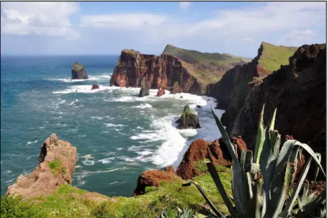
The island of Madeira is in the Atlantic Ocean, at 30o_{N and 16}o_{W, about 1000 km off the west} coast of Africa. The proposed geographical area of study corresponds to a region in the east side of the island that comprises the city of Caniçal, the surrounding mountains to its west and a portion of Ponta de São Lourenço, a long peninsula that constitutes the eastern end of the island of Madeira, to its east.

A specific focus is placed in a narrow piece of land close to the village that stretches for about 1000 m. This area, about 100 m amsl is delimited by a cliff to the north, a relatively gentle slope towards the ocean to the south, the mountainous chain to the west and the rest of the peninsula to the east. This is due to the fact that there available simulation results for this area previously obtained in [1], that can help in the validation and with which we can establish comparisons.

(22)

22

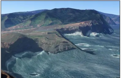
Figure 1 – Three-dimensional view of the modelled geographical area of study in the east region of the island of Madeira (north aligned with the positive direction of the y-axis).

1.2 Project structure

The structure of the document follows the chronological order in which the various steps were executed. Chapter 2 describes the characteristics of the software and the theory behind it, addressing issues such as the conservation equations, turbulence modelling and numerical and discretization techniques as well as the process of familiarization with the tools that that are part of it. Chapter 3 handles all the actions necessary to model the topography involved. In chapter 4 are depicted the preliminary steady-state simulations detailing the options taken related to domain and mesh definition, solver and boundary conditions setup and the data extraction. In chapter 5, more detailed studies are performed, using finer meshes and more accurately defined physics models, finishing with the analysis and study of the velocity and turbulence flow fields. Chapter 6 describes a transient simulation run to detect time-dependent behaviour of structures identified in chapter 5. The conclusions and future improvements to the work done are discussed in section 7. In annex A, B and C it is supplied the data extracted in sections 4, 5 and 6 respectively. Annex D contains comparative data used from [1] and in Annex E it is provided the user created code employed during the project.

(23)

23

2 ANSYS FLUENT SOFTWARE

ANSYS Inc. is an American company based in Canonsburg, Pennsylvania, founded in 1970 by John Swanson. ANSYS fluid dynamics is a product suite for modelling fluid flow. It offers fluid flow analysis capabilities, providing all the tools needed to design and optimize new fluids equipment and to troubleshoot already existing installations. The ANSYS fluid dynamics suite contains both general purpose computational fluid dynamics software and additional products to address specific industry applications. The general-purpose fluid analysis tools are the renowned ANSYS CFX and ANSYS FLUENT, the latter being the one used in this project. A wide range of physical modelling capabilities of this engineering design and analysis tool have been applied to industrial applications.

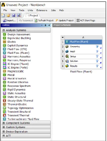
ANSYS FLUENT software is integrated into the ANSYS Workbench environment, the framework for the full engineering simulation suite of solutions from ANSYS. Within ANSYS Workbench, applications from multiple simulation disciplines can access tools common to all, such as CAD connection, two different geometry modellers (DesignModeler and SpaceClaim) and an integrated mesher. The Windows 19.1 R1 Student version of FLUENT was used in this project.

Figure 2 - General view of the Workbench environment with an open FLUENT project.

(24)

24 The author had its first contact with the software while doing an exchange semester in Universidade Técnica Federico Santa Maria in Valparaíso, Chile. The course in which that took place was called “Fundamentals of CFD” and had its last month of classes dedicated to ANSYS FLUENT. This knowledge was improved already in Portugal by studying the FLUENT learning modules provided online by the Cornell University that deal not only with theoretical concepts but also with specific case studies: laminar and turbulent flow in a pipe, boundary layer flow over a flat plate, 3D transonic flow over a wing and flow through a wind turbine blade FSI (Part 1).

All the case studies were divided in the following steps: • Pre analysis and physical concepts;

• Geometry modelling; • Mesh definition;

• Model setup including physical models’ selection, materials and boundary condition definitions, discretization techniques, convergence criteria and other solver parameters; • Simulations progress monitoring;

• 3D solutions data visualization; • 2D solutions data plotting; • Verification and validation.

Furthermore, the reading of key chapters of the software user’s and theory guide [3, 4] was essential to complement all the other learning tools.

2.1 Mathematical model

ANSYS FLUENT provides modelling capabilities for both incompressible and compressible, either laminar or turbulent fluid flow problems. Steady-state or transient analysis can be performed. For all flows, ANSYS FLUENT solves the Navier-Stokes equations for mass and momentum conservation, and for flows involving heat transfer or compressibility, an additional equation for energy conservation is also solved.

2.1.1 The mass conservation

The equation for conservation of mass, or continuity equation, can be written as follows:

𝜕𝜌

𝜕_𝑡

+ 𝛻 ∙ (𝜌𝑣⃗) = 0

(1)

Equation 1is the general form of the mass conservation equation and is valid for incompressible as well as compressible flows. The variable 𝜌 is the density and 𝑣⃗ corresponds to the vector of velocity.

(25)

25

2.1.2 The momentum conservation

Conservation of momentum in an inertial (non-accelerating) reference frame is defined by

𝜕

𝜕_𝑡

(𝜌𝑣⃗) + 𝛻 ∙ (𝜌𝑣⃗𝑣⃗) = − 𝛻𝑝 + 𝛻 ∙ 𝜏

⃗⃗⃗ + 𝜌𝑔

⃗⃗⃗⃗

(2)

where 𝑝 is the static pressure, 𝜏⃗⃗⃗ is the stress tensor (described below) and 𝜌𝑔 ⃗⃗⃗⃗ is the gravitational body force. The stress tensor 𝜏⃗⃗⃗ is given by

𝜏

⃗⃗⃗ = 𝜇(𝛻𝑣⃗ + 𝛻𝑣⃗

𝑇

)

(3)

where 𝜇 is the molecular viscosity.

2.1.3 Turbulence modelling (RANS approach)

The equations 1 and 2, also known as the Navier–Stokes equations, govern the velocity and pressure of a fluid flow. In a turbulent flow, the RANS (Reynolds-averaged Navier-Stokes) modified version of them is usually used instead. In Reynolds averaging, the solution variables in the instantaneous (exact) Navier-Stokes equations are decomposed into the mean (ensemble-averaged or time-(ensemble-averaged) and fluctuating components. For the velocity components:

𝑢

_𝑖

= 𝑢̅

_𝑖

+ 𝑢

_𝑖′

(4)

where 𝑢̅𝑖 and 𝑢𝑖′ are the mean and fluctuating velocity components (𝑖 = 1,2,3).

Likewise, for pressure and other scalar quantities:

𝜙 = 𝜙̅ + 𝜙

′

(5)

Where 𝜙 denotes a scalar such as pressure, energy, or species concentration.

Substituting expressions of this form for the flow variables into the instantaneous continuity and momentum equations and taking a time (or ensemble) average (and dropping the overbar on the mean velocity, 𝑢̅) yields the ensemble-averaged momentum equations. They can be written in Cartesian tensor form as:

(26)

26 𝜕_𝜌 𝜕_𝑡

+

𝜕 𝜕_𝑥𝑖

(𝜌𝑢

𝑖

) = 0

(6)

𝜕 𝜕_𝑡

(𝜌𝑢

𝑖

) +

𝜕 𝜕_𝑥𝑗

(𝜌𝑢

𝑖,𝑗,𝑙

𝑢

𝑗

) =

𝜕𝑝 𝜕_𝑥𝑖

+

𝜕 𝜕_𝑥𝑗

[ 𝜇 (

𝜕_𝑢𝑖 𝜕_𝑥𝑗

+

𝜕_𝑢𝑗 𝜕_𝑥𝑖

−

2 3

𝛿

𝑖𝑗 𝜕_𝑢𝑙 𝜕_𝑥𝑙

)] +

𝜕 𝜕_𝑥𝑗

(−𝜌𝑢

𝑖 ′

_𝑢

𝑗′

̅̅̅̅̅̅)

(7)

Equations 6 and 7 are called Reynolds-averaged Navier-Stokes (RANS) equations. They have the same general form as the instantaneous Navier-Stokes equations 1 and 2, with the velocities and other solution variables now representing ensemble-averaged (or time-averaged) values. Additional terms now appear that represent the effects of turbulence. These Reynolds stresses, (−𝜌𝑢̅̅̅̅̅̅), must be modelled in order to close equation 7 and that is done with 𝑖′𝑢𝑗′

turbulence models that introduce additional equations.

K-epsilon (k-ε) turbulence model is the most commonly used in CFD to simulate flow characteristics for turbulent flow conditions.

There are three variations of this model: standard, RNG and realizable.

The turbulence closure model adopted in this project is the realizable k-ε model proposed by [5]. The term realizable means that the model satisfies certain mathematical constraints on the Reynolds stresses, clarified in [4], more consistent with the physics of turbulent flows.

Both the realizable and RNG k-ε models have shown substantial improvements over the standard k-ε model where the flow features include strong streamline curvature, vortices, and rotation. It is still not clear in exactly which instances the realizable k-ε model consistently outperforms the RNG model. However, initial studies have shown that the realizable model provides the best performance of all the k-ε model versions for several validations of separated flows and flows with complex secondary flow features. It also proved to be the best turbulence model integrated in FLUENT by wind tunnel experiments in [6].

The modelled transport equations for k (turbulence kinetic energy) and ε (rate of dissipation of turbulent energy) in the realizable k-ε model are

𝜕 𝜕_𝑡

(𝜌k) +

𝜕 𝜕_𝑥𝑗

(𝜌k𝑢

𝑗

) =

𝜕 𝜕_𝑥𝑗

[(𝜇 +

𝜇_𝑡 𝜎_𝑘

)

𝜕_𝑘 𝜕_𝑥𝑗

] + 𝐺

𝑘

+ 𝐺

𝑏

− 𝜌ε − 𝑌

𝑀

(8)

(27)

27 𝜕 𝜕_𝑡

(𝜌ε) +

𝜕 𝜕_𝑥𝑗

(𝜌ε𝑢

𝑗

) =

𝜕 𝜕_𝑥𝑗

[(𝜇 +

𝜇_𝑡 𝜎_ε

)

𝜕_ε 𝜕_𝑥𝑗

] + 𝜌𝐶

1

𝑆

ε

− 𝜌𝐶

2 ε2 k+√𝜈ε

+

𝐶

_1εε k

𝐶

3ε

𝐺

𝑏

(9)

where

𝐶

1

= max [0.43 ,

𝜂 𝜂+5

] , 𝜂 = 𝑆

k ε

, 𝑆 = √2𝑆𝑖𝑗

𝑆

𝑖𝑗

(10)

In these equations, 𝐺𝑘

represents the generation of turbulence kinetic energy due to the mean

velocity gradients. 𝐺𝑏 is the generation of turbulence kinetic energy due to buoyancy. 𝑌𝑀

represents the contribution of the fluctuating dilatation in compressible turbulence to the overall dissipation rate (not considered in this work along with 𝐺𝑏) . 𝐶2 and 𝐶1ε are constants. 𝜎𝑘

and 𝜎ε

are the turbulent Prandtl numbers for k and ε, respectively.

As in other k-ε models, the eddy viscosity is computed from

𝜇

_𝑡

= 𝜌𝐶

_𝜇k2

ε

(11)

Unlike in the standard and the RNG models, the 𝐶𝜇 for the realizable is not constant and is a

function of the mean strain and rotation rates, the angular velocity of the system rotation and the turbulence fields. The notion of variable 𝐶𝜇 is well substantiated by experimental evidence.

For example, 𝐶𝜇 is found to be around 0.09 in the logarithmic layer of equilibrium boundary

layers, and 0.05 in a strong homogeneous shear flow [4].

The model constants 𝐶2, 𝜎𝑘, and 𝜎ε have been established to ensure that the model performs

well for certain canonical flow. The model constants are

𝐶

_1ε

= 1.44,

𝐶

₂

= 1.9,

𝜎

_𝑘

= 1.0,

𝜎

_ε

= 1.2

The term 𝐺𝑘, representing the production of turbulence kinetic energy, is modelled identically

for the standard, RNG, and realizable k-ε models. From the exact equation for the transport of k, this term may be defined as

𝐺

_𝑘

= − 𝜌𝑢

_𝑖′

_𝑢

𝑗′

̅̅̅̅̅̅

𝜕𝑢𝑗

(28)

28

2.2 Numerical and discretization techniques

The FLUENT solver allows the user to choose between these two numerical methods: • Pressure-based solver;

• Density-based solver.

In both cases, the finite volume method is applied in the following steps:

• Division of the domain into discrete control volumes using a computational grid; • Integration of the governing equations on the individual control volumes to construct

algebraic equations for the discrete dependent variables (“unknowns”) such as velocities, pressure, temperature, and conserved scalars;

• Linearization of the discretized equations and solution of the resultant linear equation system to yield updated values of the dependent variables.

The pressure-based approach was developed for low-speed incompressible flows but has been extended and reformulated to solve and operate for a wide range of flow conditions beyond the original intent. It is the chosen approach in our project considering that our working fluid is air that can be considered incompressible (in open systems) at velocities less than 100 m/s (Ma = 0.3) [7].

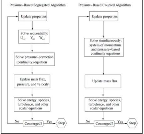
Two pressure-based solver algorithms are available in FLUENT. A segregated algorithm, and a coupled algorithm. These two are schematically explained in Figure 3.

Figure 3 – Step by step operations of a pressure-based segregated and a pressure-based coupled algorithm.

(29)

29 The segregated algorithm is memory-efficient, since the discretized equations need only to be stored in the memory one at a time but the solution convergence is relatively slow.

With the coupled algorithm, the rate of solution convergence significantly improves. However, the memory requirement increases by 1.5 – 2 times that of the segregated algorithm since the discrete system of all momentum and pressure-based continuity equations must be stored in the memory when solving for the velocity and pressure fields (rather than just a single equation, as is the case with the segregated algorithm) [3].

Within the pressure-based solver, FLUENT provides four different pressure-velocity coupling schemes, three segregated (SIMPLE, SIMPLEC and PISO) and one coupled. The SIMPLE, PISO and coupled were used alternately in this project.

2.2.1 Under-relaxation

The pressure-based solver uses under-relaxation of equations to control the update of computed variables at each iteration. This means that all equations solved using the pressure-based solver will have under-relaxation factors associated with them.

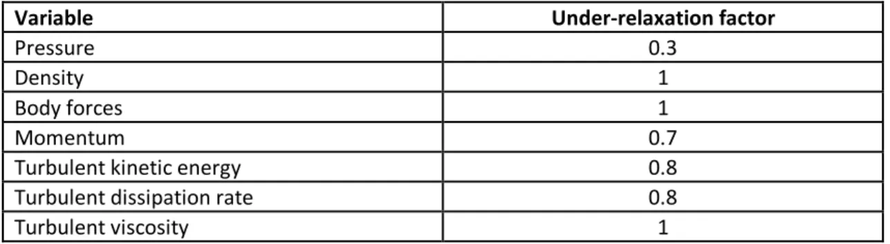
In FLUENT, the default under-relaxation factors for all variables are set to values that are near optimal for the largest possible number of cases and are defined in Table 1.

Table 1 - Default under-relaxation factors for the different variables in FLUENT.

Variable Under-relaxation factor

Pressure 0.3

Density 1

Body forces 1

Momentum 0.7

Turbulent kinetic energy 0.8

Turbulent dissipation rate 0.8

Turbulent viscosity 1

Under-relaxation reduces solution oscillations and helps to keep the computation stable. For steady-state calculations, when using the pressure-based coupled solver or the density-based implicit solver, there is the option of solving the flow in a pseudo-transient fashion. The pseudo transient under-relaxation method is a form of implicit under-relaxation.

In its turn, the warped-face gradient correction (WFGC) is designed to improve gradient accuracy for all gradient methods - cell based, node based and least squares-based gradients. WFGC is recommended for 3D simulations on polyhedral, hexahedral, and hybrid meshes (meshes containing a mix of hexahedral and polyhedral cells). WFGC computations aim to resolve gradient accuracy degradation due to very high aspect ratio, cells with non-flat faces in the boundary layer, and highly deformed cells where the formal cell centroid lies outside of the control volume.

(30)

30 Lastly, there is the high order term relaxation (HOTR). The purpose of the relaxation of high order terms is to improve the startup and the general solution behaviour of flow simulations when higher order spatial discretizations are used (higher than first). It has also shown to prevent convergence stalling in some cases. Such high-order terms can be significant in certain cases and lead to numerical instabilities [3].

2.2.2 Convergence criteria

At the end of each solver iteration, the residual sum for each of the conserved variables is computed and stored. On a computer with infinite precision, these residuals will go to zero as the solution converges. On an actual computer, the residuals decay to some small value (“round-off”) and then stop changing (“level out”).

For single-precision computations (the default for workstations and most computers), residuals can drop as many as six orders of magnitude before hitting round-off. Double-precision residuals can drop up to twelve orders of magnitude [4]. The unscaled residual, summed over all the computational cells P, computed by FLUENT pressure-based solver can be written as

𝑅

𝜙

= ∑

_{𝑐𝑒𝑙𝑙𝑠 𝑃}

|∑

_𝑛𝑏

𝑎

_𝑛𝑏

𝜙

_𝑛𝑏

− 𝑎

_𝑃

𝜙

_𝑃

|

(13)

Where 𝜙 is a general variable, 𝑎𝑃 the center coefficient and 𝑎𝑛𝑏 the influence coefficients for

the neighbouring cells. In general, it is difficult to judge convergence by examining the residuals defined by equation 13 since no scaling is employed. ANSYS FLUENT scales the residuals using two kinds of scaling factors, representative of the flow rate of 𝜙 through the domain. The factors are termed global scaling and local scaling. The globally scaled residual is defined as

𝑅

𝜙

=

∑𝑐𝑒𝑙𝑙𝑠 𝑃 |∑𝑛𝑏𝑎𝑛𝑏𝜙𝑛𝑏 − 𝑎𝑃𝜙𝑃|

∑𝑐𝑒𝑙𝑙𝑠 𝑃 |𝑎𝑃𝜙𝑃|

(14)

For the momentum equations the denominator term 𝑎𝑃𝜙𝑃 is replaced by 𝑎𝑃𝑣𝑃, where 𝑣𝑃 is the

magnitude of the velocity at cell P. The locally scaled residual is defined as

𝑅

_𝜙

=

√∑ (1 𝑛) 𝑛 𝑐𝑒𝑙𝑙𝑠 ( ∑_𝑛𝑏_{𝑎𝑛𝑏𝜙𝑛𝑏 − 𝑎𝑃}_𝜙𝑃 𝑎𝑃 ) 2 (𝜙𝑚𝑎𝑥− 𝜙𝑚𝑖𝑛)𝑑𝑜𝑚𝑎𝑖𝑛

(15)

As in global scaling, for the momentum, 𝜙 is replaced by 𝑣𝑃 of the cell. The scaled residual is a

more appropriate indicator of convergence for most problems. For the continuity equation, the unscaled residuals for the pressure-based solver are defined as

(31)

31 𝑅𝑐 _{= ∑} _{|𝑟𝑎𝑡𝑒 𝑜𝑓 𝑚𝑎𝑠𝑠 𝑐𝑟𝑒𝑎𝑡𝑖𝑜𝑛 𝑖𝑛 𝑐𝑒𝑙𝑙 𝑃|}

𝑐𝑒𝑙𝑙𝑠 𝑃

(16)

The local scaling is the same for all equations. However, the global scaling treats continuity in a different way and it is defined as

𝑅_{𝑖𝑡𝑒𝑟𝑎𝑡𝑖𝑜𝑛 𝑁}𝑐

𝑅_{𝑖𝑡𝑒𝑟𝑎𝑡𝑖𝑜𝑛 5}𝑐

(17)

The denominator is the largest absolute value of the continuity residual in the first five iterations. The scaled residuals described above are a useful indicator of solution convergence. There are no universal metrics for judging convergence. Residual definitions that are useful for one class of problem are sometimes misleading for other classes of problems. Therefore, it is a good idea to judge convergence not only by examining residual levels, but also by monitoring relevant integrated quantities such as the drag.

For most problems, the default convergence criterion in FLUENT is enough. This criterion requires that the globally scaled residuals, defined by equation 14 decrease to 10−3 for all equations except the energy equation for which the criterion is 10−6. Locally scaled residuals defined by equation 15 should decrease to 10−5_{for all equations.}

(32)

(33)

33

3 TOPOGRAPHY MODELLING

The topographical map of the area supplied was extracted from the Global Digital Elevation Map, a tool available online and provided by NASA. This map consists of a set of discrete points with contour heights at every 28m. These points, 2628477 in total, represented by its UTM coordinates in .xyz file format, comprise an area of 40x50km centred in the east half part of the island of Madeira.

Such a big amount of data is unnecessary as in this study only the region of interest and its surrounding areas (defined in Figure 1) matter. Therefore, it was reduced to an area of 5x12 km using Microsoft Excel. The points were also displaced evenly in a way that to the origin of the domain ended up corresponding a (x,y,z)= (0,0,0). The next step was trying to connect all the points and create a surface out of them. After extensive research on how to do it using the geometry modelling tools provided by FLUENT, no solution was found so, there was a need to resort to external software.

For this purpose, the most suitable to be found was MeshLab 2016.12, an open source system that offers features for processing raw data produced by 3D digitalization tools/devices and for preparing models for 3D printing. It provides a set of tools for editing, cleaning, healing, inspecting, rendering, texturing and converting meshes. It is also used for processing and editing 3D triangular meshes.

The points were imported into the software, and two filters were applied sequentially: Compute normals for point sets and Screened Poisson Surface Reconstruction described in Figure 4.These filters transformed the discrete set of points into a continuous surface recreating the intended geometry.

Figure 4 – Description of Compute normals for point sets and Screened Poisson Surface Reconstruction filters and parameters applied.

(34)

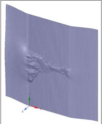
34 The surface was exported as a .stl file. An .stl file describes a raw, without texture and color, unstructured triangulated surface by the unit normal and vertices (ordered by the right-hand rule) of the triangles using a three-dimensional Cartesian coordinate system. It was then imported into SpaceClaim used throughout the whole project to the detriment of DesignModeler because, during the familiarization with both, it was found to be more prepared to deal with complex and irregular geometries.

The aspect of the imported surface can be seen in figure 5.The curved surfaces that delimit the central region to the right and to the left were automatically added after applying the Screened Poisson Surface Reconstruction filter so they had to be trimmed.

An analysis of the geometry revealed some defective details that might seem insignificant but were found worth of rectifying. A visualization of photos of the region (Figure 6) together with Google Earth perspectives, shows that the north cliffs that surround the land surface are steep and do not have sediment accumulation at the base.

Figure 5 – Aspect of the geometry .stl file when imported into SpaceClaim (north aligned with the

(35)

35 Nevertheless, in the geometry obtained it is found that there are represented significant areas of terrain at the bases of the north cliffs (Figure 7) and not at the south ones (Figure 8).

Figure 8 – Part of the south cliffs of the land surface in SpaceClaim. Figure 6 – Cliffs that delimit the north border of the land surface.

Figure 7 – Part of the north cliffs of the land surface in SpaceClaim (defective details within the black contour, islets marked with green crosses).

(36)

36 The visualization of 3D images of Google Earth allowed to raise a probable hypothesis for this fact. In Figure 9, it is possible to see that the waves hitting the north cliff are huge and look captured as an extension of land. This theory also explains why this phenomenon does not occur in the south cliffs as the waves come predominantly from north.

The obtention of data by the Global Digital Elevation Map is also done by satellite so it could be also affected by these irregularities. In fact, in the website of the Global Digital Elevation Map it is mentioned: “However, users are advised that the data contains anomalies and artifacts that will impede effectiveness for use in certain applications”.

Considering all of this and using SpaceClaim, the problematic areas were removed and so were the islets that can be seen in Figure 6 and Figure 7 as they do not significantly interfere in the flow and would increase a lot the complexity of the geometry.

After this, the faceted data, all the surface subdivisions seen in Figure 7 and Figure 8, had to be transformed into surface patches defining the sea and land regions. To do this, SpaceClaim has a powerful tool of reverse-engineering called Skin surface that even allows the user to control the precision with which the terrain details are captured by controlling the number of Samples. To finish the geometry modelling, the three surfaces (two for the sea and one for land) are stitched together into a single surface body using the feature Stitch and its edges are extruded to create the faces in which the lateral boundary conditions will be applied. The ceiling of the box is created by using the feature Fill and with this closure, it is automatically created an interior volume for our flow. Finally, the geometry is ready to be meshed.

In figure 11, it is possible to see a representation of the box. More than one variation of it was made with different number of Samples, different heights and different distances from the north and south boundary in relation to land.

Figure 9 – Aspect of the north cliffs of the land surface in Google Earth.

(37)

37

4 PRELIMINARY STEADY-STATE SIMULATIONS

Having defined the general geometry of our model, the main objective of the first round of steady-state simulations was to establish the limits of the integration domain height and to have an initial idea of the flow field. Therefore, the result analysis is much more qualitative than quantitative.

4.1 Geometry, domain and meshing

The domain height was defined as 1500 m in [1] but it was decided to evaluate how its increase could affect the quality of the simulation. Simulations were performed for five different heights: 1500 m, 2000 m, 2500 m, 3000 m and 3500 m.

In terms of width, namely range of Eastings, it was kept approximately equal to [1] with the UTM extending between 335000 m to 340000 m. In terms of length, namely range of Northings, it was slightly increased in these first simulations when compared to [1], in order to avoid rebounding of flows, artificial accelerations and other negative effects, extending between 3618000 m to 3631060 m.

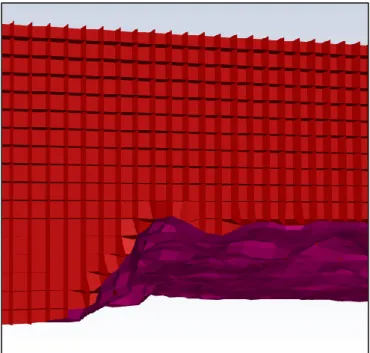
With the help of the integrated mesher of FLUENT, a structured mesh was created for each situation, using the Cartesian method that creates mainly orthogonal hexahedral cells. The approximate face length of each is 90 m. No refinements of the mesh were done at this phase. Table 2 shows the number of cell elements for each case and in Figure 10 a detailed view of one of the meshes is displayed.

Table 2 – Number of cell elements for each integration domain with a different height.

Height [m] Cell elements

1500 136959

2000 189498

2500 219203

3000 252132

(38)

38

4.2 Setup configuration

The following step was to open the setup menu that allows us the definition of several specifications (physical models, boundary conditions, discretization schemes, under relaxation factors, residuals monitoring, etc) of the simulation and to perform the calculations.

Before the setup menu opens, a window pops, and in between many other things, allows us to choose between single/double precision and serial/parallel processing. Double precision and serial were the options chosen. The FLUENT serial solver manages file input and output, data storage, and flow field calculations using a single solver process on a single computer.

The turbulence model chosen for this project was the realizable k-ε, in section 2.1.3, with the default constant values. Since we considered the flow incompressible and there was no interest in evaluating the temperature fields, the energy equation was kept turned off. The atmospheric air was modelled with 𝜌 = 1.225 𝑘𝑔/𝑚3.

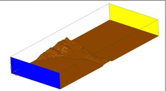
For each face of the integration domain (Figure 11), the following boundary conditions were assigned:

• North face (yellow): velocity inlet boundary, considering a constant velocity magnitude of 30 m/s, normal to the face;

• South face (blue): outflow boundary, through which the flow exits the domain;

• Ground face (brown): wall boundary, imposing the no-slip condition and forcing the creation of a boundary layer;

• Top, East and West faces (transparent): wall boundary, imposing a complete slip condition with a specified shear stress of zero in all directions.

Figure 10 – Detailed view of the hexahedral mesh showing the elements that define the interior fluid (red) and the land surface

(39)

39

The previously mentioned increase in the domain length in section 4.1 was also done to make sure that the flow at the outlet boundary was as close as possible to being fully developed, condition recommended by FLUENT to apply an outflow boundary condition. However, outflow boundaries can also be defined at physical boundaries where the flow is not fully developed - and that can be done with confidence if the assumption of a zero-diffusion flux at the exit is expected to have a small impact on the flow solution.

The zero-diffusion flux condition applied at outflow cells means that the conditions of the outflow plane are extrapolated from within the domain and have no impact on the upstream flow. It is important to note that gradients in the cross-stream direction may exist at an outflow boundary. Only the diffusion fluxes in the direction normal to the exit plane are assumed to be zero.

The wall functions used in the ground face were the standard, based on the proposal of [8] and modified for roughness as detailed in FLUENT User’s guide. The roughness constant was kept at the default value of 0.5 and the roughness heights, z0, were taken from [1] to be 0.03 m and 0.0002 m for land and sea surfaces respectively. The pressure-velocity coupling scheme adopted was the coupled, in section 2.2, with the method of spatial discretization for each variable defined in table 3.

Table 3 – Spatial discretization methods for each variable used in the preliminary simulations.

Variable Method

Gradient Least squares cell based

Pressure Second order

Momentum Second order upwind

Turbulent kinetic energy First order upwind

Turbulent dissipation rate First order upwind

Figure 11 – One of the integration domains used in the preliminary simulations with colour coded boundaries.

(40)

40 Additionally, the three under relaxation methods mentioned in section 2.2.1 were turned on: pseudo-transient, warped-face gradient correction and high order term relaxation.

The problem was started with a hybrid initialization. A hybrid initialization is a collection of recipes and boundary interpolation methods. It solves Laplace's equation to determine the velocity and pressure fields. All other variables, such as temperature, turbulence, and so on, are automatically patched based on domain averaged values.

For each integration domain case with a different height, 300 iterations were performed. The solver stopping criteria were setup as the default for globally scaled residuals mentioned in section 2.2.2. As soon as continuity, x, y and z momentum, k and ε globally scaled residuals reach the value of 10−3, the solution stops.

4.3 Results extraction and analysis

The setup menu has its own resources to extract graphics, plots and reports of different variables of interest. After each set of iterations, by default, a plot of the globally scaled residuals of the conservation equations per iteration is provided. These plots will be used to analyse convergence. Nevertheless, FLUENT has a much better tool for the intended purpose called CFD-Post.

CFD-Post is a post-processor integrated in the Workbench environment, designed for extracting and aiding the analysis of data. Considering that the objective of this round of simulations was to define the height of the domain, two types of information were extracted:

• 2D contour graphics of the velocity magnitude 10 m under the top face to evaluate how close the flow gets to the free-stream velocity in each situation and, therefore, how appropriate was the use of the complete slip boundary condition (velocity vectors tangential to the face). It was evaluated 10 m under the faces because they are not 100% straight and orthogonal between them so in some situations there were not values exactly over them;

• 2D contour graphics of the velocity magnitude at a height of 190 m amsl to evaluate how the upper limit distance affects the flow characteristics in a plane slightly above the region of interest.

All the data extracted is condensed in ANNEX A. The analysis of the values of the residuals in section 9.1, from Figure 36 to Figure 40, reveals that for every case, they stabilized very quickly (around 30 iterations).

Also, it is noted that there was a slight decrease in the residuals for all equations with the increase in the integration domain height, apart from continuity. The oscillation around the mean stabilized value also decreased with the increase of the domain height. All the residuals, apart from continuity and k, descended under the values defined for convergence criteria. The high coarseness of the mesh due to the absence of refinement in the more complex parts of the geometry may be an important contributor to the undesirable high values for the residuals of continuity and k.

(41)

41 A more specific explanation for the high values of continuity residual may lie in equation 17. The scaling factor (denominator) of the globally scaled residual of continuity, unlike in all the others, is the largest absolute value of the continuity residual in the first five iterations.

This means that if the hybrid initialization applied in this simulation leads to a good initial guess of the flow field, the initial continuity residual may be very small leading to a large scaled residual for the continuity equation. In such a situation it is useful to examine the unscaled residual and compare it with an appropriate scale, such as the mass flow rate at the inlet.

Considering the objectives of this first round of simulations, the results were deemed acceptable and no further monitoring instruments were introduced.

The analysis of the graphic contours in section 9.2, from Figure 41 to Figure 45, showed that for each 500 m increase of the domain height, the velocity magnitude close to the upper limit above the zone of influence of the big west mountainous chain (the one that causes the biggest disruption of the flow) decreased almost 1 m/s, going from a value around 36 m/s to around 32 m/s. Also, the flow field got increasingly more uniform approaching the value of the free-stream velocity, defined at the inlet as 30m/s.

The analysis of the graphic contours in section 9.3, from Figure 47 to Figure 50, is intended not to focus on the characteristics of the flow but on its variations with the increase of the domain height. There is not a clear pattern of variations unless in the disappearance of the low velocity zones leaning on the east boundary for the 3500 m and 3000 m domain heights. For these two bigger domain heights, the flow variations in between them also seemed more negligible. Although the viewing conditions are similar for all cases, to each increase of the integration domain height it did not correspond a proportional increase of the number of cell elements due to limitations in the controls of the mesher and that might imply inherently different structures. Taking into account all the previous considerations and in an attempt to find a balance between precision and a reasonable domain size, the defined domain height for the simulations that followed was 2500 m.

In Figure 51, as a complement, there is a 2D graphic contour of the velocity w component 2490 m amsl for a domain height of 2500 m and as expected, it is negligible.

(42)

(43)

43

5 STEADY-STATE SIMULATIONS

After enough background knowledge was acquired and variables such as the domain height fixed, more detailed steady-state simulations were performed. The characteristics of the flow field were now able to be analyzed and compared with the results of [1].

Several different configurations were tried in order to perceive ways to reach the desired results faster and to achieve greater reliability. Simulations with northerly (north-prevailing) winds were done first, in section 5.3.1, experimenting with both the SIMPLE and coupled methods and two different outlet boundary conditions: outflow and pressure outlet. Simulations with southerly (south-prevailing) winds followed, in section 5.3.2, using the method and outlet boundary condition considered most successful when simulating with northerly winds.

Due to the low altitude, the size of the integration domain and the relatively high wind speeds considered, both the stratification and the Coriolis effects were ignored. All the settings not mentioned on the following subsections are assumed not to have changed from the previous round of simulations.

5.1 Geometry, domain and meshing

Based on the procedures mentioned in chapter 3, the geometry of the land surface was improved by increasing the number of Samples applied with the Skin surface feature. Two different integration domains were created to be used by the simulation with the northerly and the southerly winds. For the northerly simulations, the inlet is in the north face and the outlet in the south face, whereas for the southerly it swaps. The length of each integration domain was adjusted so that the distance from the inlet and from the outlet to land was 1000 m and 2500 m respectively. The value of 1000 m was estimated to be the necessary to let the logarithmic velocity profile applied at the inlet (defined in 5.2.1) to adjust and fully develop before reaching land. The value of 2500 m was estimated to be the necessary to let the flow fully develop after crossing the land surface and before reaching the outlet, a condition that FLUENT recommends when using the outflow boundary condition as mentioned in 4.2.

The land surface was divided in three patches so that the region of interest could be more easily refined during the meshing process. This process was carried out in such a way as to make the most of the mesher's abilities that limit the number of cell/node elements to 512000 elements in the FLUENT Student license.

(44)

44 The focus was placed in the region of interest but without neglecting much of the rest of the land's surface since it was also intended to observe the characteristics of the flow in some detail in those areas. This time, it was decided to use tetrahedral elements whose size decreased in the upper direction and towards the borders. A face sizing feature was applied on the two patches of land surface outside the region of interest and on the upstream section of the sea defining the size of its elements as 60 m (maximum size on the face), another was applied in the region of interest with elements of 25 m.

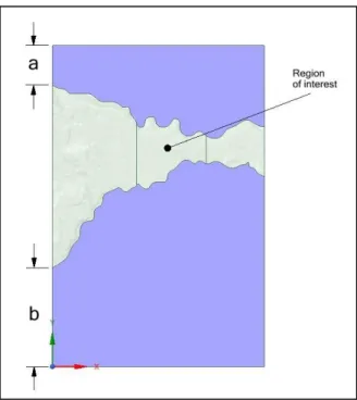
Figure 12 – View from above of one of the geometries before being meshed. The blue region corresponds to the sea. a) distance from north face to land b)

distance from south face to land.

Figure 13 – View of the land surface after being meshed with a greater refinement on the region of interest (darker).

(45)

45 An inflation feature was spread throughout the entire ground surface, including sea and land, defining 8 layers with a growth rate of 1.3 and a height of the first element near the ground of 2 m.

The high complexity of the land surface geometry meant that it was not possible, without losing too much detail and using the integrated mesher, to obtain a more structured mesh that usually guarantees faster solutions with better accuracy. Nevertheless, to control the quality of the mesh, the main and most important metrics were evaluated, namely, the skewness and the orthogonal quality of the cell elements. FLUENT recommends that the skewness does not exceed the value of 0.95 in any cell and that the worst value of orthogonal quality should be superior to 0.01. In table 4, the two variables are rated according to their range of values. In table 5, the values obtained for the two meshes are presented.

Table 4 – Mesh metrics ratings according to a range of values.

Skewness

Outstanding Very good Good Sufficient Bad Inappropriate

0-0.25 0.25-0.50 0.50-0.80 0.80-0.95 0.95-0.98 0.98-1.00

Orthogonal quality

Inappropriate Bad Sufficient Good Very good Outstanding

0-0.001 0.001-0.15 0.15-0.20 0.20-0.70 0.70-0.95 0.95-1.00

(46)

46

Table 5 – Mesh metrics values obtained for the integration domains used in the northerly and southerly winds simulations.

Northerly Southerly

Average skewness 0.24 0.23

Maximum skewness 0.81 0.66

Average orthogonal quality 0.76 0.76

Minimum orthogonal quality 0.14 0.25

Cell elements 501830 502362

The recommended values were not exceeded, and the average values can be labelled as outstanding for skewness and very good for orthogonal quality.

5.2 Setup configuration

Following the opening of the setup menu, it was once again chosen the option for double precision but this time it was decided to adopt a parallel processing.

FLUENT parallel solver allows the computation of a solution by using multiple processes that may be executing on the same computer, or on different computers in a network. It splits up the grid and data into multiple partitions, then assigns each grid partition to a different compute process (or node). The machine used was an OMEN HP laptop with an Intel® Core™ i5-6300HQ processor of 4 cores, so 4 processes (partitions) were defined and each one assigned to a different core, therefore enhancing the performance of the calculations.

5.2.1 Inlet

The velocity inlet boundary was now defined with a logarithmic boundary layer profile, with an height of 𝛿=1000 m and a free-stream velocity equal to 11.6 m/s as in [1].

Perfect velocity entry profiles are difficult to define but good approximations can be used to minimize adaptation in the initial part of the domain. The velocity profile used was defined by the following equations:

𝑢(𝑧) = (𝑢∗ 𝜅

) log (

𝑧+ 𝑧₀ 𝑧0

) 𝑓𝑜𝑟 𝑧 ≤ 𝛿

(18)

𝑢(𝑧) = (

𝑢∗ 𝜅

) log (

𝛿+ 𝑧₀ 𝑧0

) 𝑓𝑜𝑟 𝑧 > 𝛿

( 19)

(47)

47

k =

𝑙𝑚2 𝐶_𝜇1/2

(

𝑢_∗ ℒ

)

2

(20)

ε = 𝑙

_𝑚2

(

𝑢∗ ℒ

)

3

(21)

where 𝑙𝑚 = 𝑚𝑖𝑛{𝜅(𝑧 + 𝑧0), 𝐶𝜇𝛿)}, and ℒ = 𝜅(𝑧 + 𝑧0) if 𝑧 < 𝛿 or ℒ = 𝛿, if 𝑧 ≥ 𝛿.

The variable 𝑢 is the longitudinal velocity normal to the inlet and 𝜅 is the von Kármán constant equal to 0.4. The value of 𝑧0 was defined as 0.0002 m (sea region) as already done in 4.2.

The friction factor, 𝑢∗, was assumed to have the value of 0.3 m/s in order to achieve the intended

free-stream velocity of 11.6 m/s. Although the 𝐶𝜇 is not constant in the realizable k-ε model as

mentioned in 2.1.3, the FLUENT’s default value of 0.09 for the standard and RNG models can be accepted for the realizable in inertial sublayers in an equilibrium boundary layer. Therefore, it was accepted in this case.

Unfortunately, to the date, FLUENT has no automatic way of implementing these functions in the boundaries but it allows the user to define a UDF, user-defined function, a C function that can be dynamically loaded within the solver to enhance its standard features. UDFs are defined using DEFINE macros provided by ANSYS. After being interpreted or compiled, UDFs become visible and selectable in FLUENT dialog boxes and can be hooked to the solver by choosing the function name in the appropriate dialog box. Several examples of UDFs are presented in [9] and were easily adapted to model the equations 18, 19, 20 and 21. The code is made available in ANNEX E.

5.2.2 Wall functions

After using the standard wall functions in the preliminary simulations, in chapter 4, this time, it was chosen a different wall treatment for the ground face. The choice fell on the scalable wall functions. Scalable wall functions avoid the deterioration of standard wall functions under grid refinement below 𝑦∗< 11. The variable 𝑦∗_{is the dimensionless normal distance to the wall}

defined in FLUENT as:

𝑦

∗

=

𝜌𝑦𝑃(√𝐶𝜇 1/2

𝑘)

𝜇

(22)

where 𝑦𝑃 is the distance of the cell centroid to the wall and 𝑘 is the turbulent kinetic energy.

These wall functions produce consistent results for grids of arbitrary refinement. For grids that are coarser than 𝑦∗> 11 , the standard wall functions are identical. The use of standard equilibrium and non-equilibrium wall functions implies that the near-wall grid node resides entirely within the log-law region, but this can be difficult to realise in general applications.

Computational simulation of a flow over the east part of the Madeira island