i
Spatial-Temporal Crop Yield Analysis
in East Kalimantan, Indonesia
Spatial disaggregation of crop yield data and
estimation of future production
Spatial-Temporal Crop Yield Analysis in East Kalimantan,
Indonesia
Spatial disaggregation of crop yield data and estimation of future
production
Dissertation supervised by Prof. Dr. Judith Verstegen
Institute for Geoinformatics
Westfälische Wilhelms-Universität, Münster, Germany
Co-supervised by Dr. Filiberto Pla
Dept. Lenguajes y Sistemas Informaticos Universitat Jaume I, Castellón, Spain
Dr. Carina van der Laan Self-employed advisor and researcher
Sustainable Forested Landscapes
ii
Spatial-Temporal Crop Yield Analysis
in East Kalimantan, Indonesia
spatial disaggregation of crop yield data and
estimation of future production
Spatial-Temporal Crop Yield Analysis in East Kalimantan, Indonesia
spatial disaggregation of crop yield data and estimation of future
production
Dissertation supervised by Prof. Dr. Judith Verstegen
Institute for Geoinformatics
Westfälische Wilhelms-Universität, Münster, Germany
Co-supervised by Dr. Filiberto Pla
Dept. Lenguajes y Sistemas Informaticos Universitat Jaume I, Castellón, Spain
Dr. Carina van der Laan Self-employed advisor and researcher
Sustainable Forested Landscapes
DECLARATION
I, Muhammad Wakhid Pramujati master student of the Geospatial Technology Erasmus Mundus program, aware of my responsibility of the penal law, declare and certify with my signature that my thesis entitled
Spatial-Temporal Crop Yield Analysis in East Kalimantan, Indonesia
spatial disaggregation of crop yield data and estimation of future production
is entirely the result of my own work I have faithfully and accurately cited all my sources, including books, journals, handouts and unpublished manuscripts, as well as any other media, such as the Internet, letters or significant personal communication.
I understand that
- literal citing without using quotation marks and marking the references - citing the contents of a work without marking the references
- using the thoughts of somebody else whose work was published, as of our own thoughts are counted as plagiarism. I declare that I understood the concept of plagiarism and I acknowledge that my thesis will be rejected in case of plagiarism.
Münster, 23rd February 2018
Signature of thesis writer
1
Spatial-Temporal Crop Yield Analysis in East Kalimantan, Indonesia
spatial disaggregation of crop yield data and estimation of future production Abstract
As the largest agricultural country in South East Asia, Indonesia possesses enormous agriculture resources. In the last decade, the Government of Indonesia has focused on the production development of 4F crops, meaning crops for the production of Food, Feed, Fiber, and Fuel. In 2014, Indonesia had about 101 million hectares agricultural land which comprised of approximately 47 million hectares cultivated area and the remaining 54 million hectares were expandable agriculture lands. However, the expansion has to consider Indonesia Law No. 44 in Year 2009 (Undang – Undang No 4 Tahun 2009) regarding the security of sustainable food cropland that restricts the conversion of food cropland into timber forest, industry or settlements. In fact, unwanted land use land cover (LULC) change happened due to the excessive expansion of oil palm, rubber, pulpwood and mining industries particularly in East Kalimantan. Two districts that exhibit significant LULC change are Kutai Barat and Mahakam Ulu. An additional 78.5 thousand ha of rubber, 31 thousand ha of oil palm and 23.6 thousand ha of pulpwood plantations have dominated the LULC change in Kutai Barat and Mahakam Ulu districts from 1990 to 2009. Although in general, the agricultural expansion has become the main cause of unwanted LULC change and forest cover loss, these have also contributed to positive economic benefit. In order to evaluate the economic benefit of historic agricultural expansion as well as to estimate the economic benefit of future agricultural expansion, it is necessary to look thoroughly at the geographic distribution of crop yields within the districts because we would like to understand the crop yield for every agriculture production area. The issue on the existing crop statistic data is that the crop statistics are conveyed as tabular-based data and reported at the national, provincial or district level of detail. Thus, examining crop distribution in district level is certainly challenging. Hence, a spatial crop yield allocation model was applied to generate pixel-level crop yield representation of Kutai Barat and Mahakam Ulu districts in 2000 and 2009 based upon available the regional crop statistics data and the existing LULC maps and further analyze its spatial-temporal pattern within this period of time. Furthermore, an evaluation of crop yield production and the agriculture
2 expansion trend from 2000 to 2009 were applied to a 2030 land use projection from a land use change model to project the pixel level crop yield in 2030. Between 2000 and 2009, rubber plantation exhibits land expansion and followed by the increase of yield. While the expansion of oil palm in 2009 is followed by the degradation of yield. We presume this due to the oil palm plantation in 2009 is still in early harvesting stage. The accuracy of disaggregation model is highly depending on the quality of data particularly crop statistic data and LULC map. The deviation between these two data leads to the occurrence of a high error in disaggregation results. By estimating oil palm and rubber yield based on projected LULC maps in 2030, the future expansion is suggested to follow the Limited Unrestricted scenario since this scenario is able to provide highest average yield with relatively small area among other scenarios. In this manner, either government or people in Kutai Barat and Mahakam Ulu are able to gain optimal agricultural benefit without sacrificing an excessive number of land resources.
Keywords: Crop yield; agriculture expansion; oil palm; rubber; spatial production allocation model; East Kalimantan
3 ACKNOWLEDGEMENT
First and foremost, I would like to express my sincerest gratitude to my supervisor, Prof. Dr. Judith Verstegen, who has supported me throughout my thesis starting from the research topic discussion, the proposal development and finally until this research works have finished with her patience, motivation, and immense knowledge. My indebtedness also goes to my co-supervisors, Dr. Carina van der Laan and Dr. Filiberto Pla for their ideas, suggestions and comments all the time during the all processes. I could not have imagined having better supervisors and mentors for my master theses.
Second of all, I am fully grateful granted as an EU-Erasmus Mundus fellowship scholar. Without this fellowship, I would have never imagined having a chance to pursue master education in Europe. This very opportunity has granted an answer to my younger self-curiosity about how does it feel to live in European Countries how snow really looks like. As a kid, I was always only dreaming about building a snowman, throw a snowball and get slipped over the snowy pavement which will never happen in my lovely tropical home country.
I would like to take this opportunity to express my greatest gratitude to all my professors particularly from NOVA IMS Univeside Nova de Lisboa (UNL) and Institut für Geoinformatik (IFGI) Universität Münster for all academic effort to enrich my knowledges, experiences and skill during this master. Master of Geospatial Technologies program really broaden and foster my knowledges which I gained from my late education as geodetic surveyor and make me realize how broad is the world of geospatial, how countless things can be done and motivate me to keep learning.
I dedicate this work to my dearest lady and my son, Wahyuningrum Angesti and Abimanyu Terangbhumi. I thankful for both of them who always be my very motivation throughout all processes. Special thanks to Allah SWT who has showed me all priceless chances and graces all this time.
4 ACRONYMS
ANOVA
Analysis of Variance
BPS
Badan Pusat Statistic
CPO
Crude Palm Oil
FAO
Food and Agriculture Organization of the United Nations
GAEZ
The Global Agro-Ecological Zones
HPH
Hak Pengusahaan Hutan
HTI
Hutan Tanaman Industri
IIASA
The International Institute for Applied Systems Analysis
LULC
Land Use and Land Cover
MLS
Multivariate Least Square
OLS
Ordinary Least Square
PLUC
PCRaster Land Use Change Model
REPELITA
Rencana Pembangunan Lima Tahun
SEA
South East Asia
SPAM
Spatial Production Allocation Model
Tukey-HSD
Tukey Honestly Significant Difference
5 TABLE OF CONTENTS ABSTRACT ... 1 ACKNOWLEDGEMENT ... 3 ACRONYMS ... 4 LIST OF TABLES ... 6 LIST OF FIGURES ... 7 1 INTRODUCTION ... 10 1.1 Objectives ... 10 1.2 Research Questions... 11 1.3 Theses Structure ... 11 2 METHODS ... 12 2.1 Study Area ... 12
2.2 Spatial Production Allocation Model ... 15
2.3 Crop Yield Disaggregation Processes Applied to Kutai Barat and Mahakam Ulu Case ... 17
2.4 Determination of Suitability Indexes for Oil Palm and Rubber ... 19
2.5 Cross Validation ... 20
2.6 Least Square-Based Estimation of Crop Yields ... 21
2.7 Significant Test of ANOVA and Tukey HSD Post-Hoc Analysis ... 22
3 DATA ... 24
3.1 Crop Statistic Data and Districts Administrative Boundaries ... 24
3.2 Land Use and Land Cover Map ... 27
3.3 Crop-Specific Biophysical Suitability Map ... 28
3.4 Irrigation Map ... 30
3.5 Projected Land Use and Land Cover Map ... 31
4 RESULTS AND DISCUSSIONS ... 33
5 CONCLUSIONS... 46
APPENDICIES ... 49
6 LIST OF TABLES
TABLE 1. THE NULL HYPOTHESIS OF TUKEY HSD ON THE SIX SAMPLE PAIRS OF
ESTIMATED OIL PALM AND RUBBER YIELDS IN 2030 PROJECTED LULC SCENARIOS ..24 TABLE 2. SUB-DISTRICTS RUBBER PRODUCTION AND CROPPING AREA OF KUTAI BARAT
AND MAHAKAM ULU IN 2009) ...25 TABLE 3. DISTRICT’S CROP PRODUCTION AND CROPPING AREA OF EAST KALIMANTAN IN
2000 AND 2009 ...26 TABLE 4. ACTUAL LAND USE AND LAND COVER IN 1990, 2000, 2009 AND PROJECTED LULC
IN 2030 OF KUTAI BARAT AND MAHAKAM ULU ...32. TABLE 5. THE PRODUCTION, CROPPING AREA AND AVERAGE YIELDS OBTAINED FROM
THE ESTIMATED YIELDS OF KUTAI BARAT AND MAHAKAM ULU IN 2030 UNDER FOUR PROJECTED LULC SCENARIOS ...44 TABLE 6. TUKEY-HSD POST-HOC TEST RESULT OF ESTIMATED OIL PALM AND RUBBER
7 LIST OF FIGURES
FIGURE 1. LOCATION OF KUTAI BARAT AND MAHAKAM ULU DISTRICTS IN EAST
KALIMANTAN IN INDONESIA ...13 FIGURE 2. CROP YIELD DISAGGREGATION ILLUSTRATION WITHIN AN AGRICULTURE
BOUNDARY ACCORDING TO THE SPAM METHOD ...16 FIGURE 3. SPATIAL PRODUCTION ALLOCATION MODEL (SPAM) APPLICATION AND
ESTIMATION FUTURE CROP IN KUTAI BARAT AND MAHAKAM ULU CASE ...18 FIGURE 4. DETERMINATION PROCESS OF OIL PALM AND RUBBER SUITABILITY INDEXES
AND SUITABILITY MAP OF KUTAI BARAT AND MAHAKAM ULU CREATION
WORKFLOW ...20 FIGURE 5. LAND USED AND LAND COVER MAPS OF KUTAI BARAT AND MAHAKAM ULU
2000 AND 2009 ...27 FIGURE 6. THE INTERMEDIATE-IRRIGATED OIL PALM , THE INTERMEDIATE-RAINFED OIL
PALM, AND INTERMEDIATE- RAINFED RUBBER SUITABILITY MAPS OF KUTAI BARAT AND MAHAKAM ULU OBTAINED FROM GAEZ DATA SET ...29 FIGURE 7. IRRIGATION AREA OF KUTAI BARAT AND MAHAKAM ULU BASED ON GLOBAL
IRRIGATION MAP ...31 FIGURE 8. THE PROJECTED LULC MAPS OF KUTAI BARAT AND MAHAKAM ULU IN 2030 AS
RESULT OF THE PLUC SIMULATION MODEL UNDER THE FOUR ALLOCATION ZONING POLICIES AND LAND USE DEMAND DEVELOPMENT SCENARIOS ...33 FIGURE 9. MODIFIED SUITABILITY MAPS OF OIL PALM AND RUBBER FOR WHOLE AREA OF
KUTAI BARAT AND MAHAKAM ULU, BASED ON THE LULC MAP IN 2000 AND 2009 , WATER SUPPLY SYSTEMS, INPUT LEVEL, AND CROP TYPES ...34 FIGURE 10. THE DISAGGREGATED OIL PALM AND RUBBER YIELDS OF KUTAI BARAT AND
MAHAKAM ULU IN 2000 AND 2009 AS RESULTS OF THE SPAM DISAGGREGATION METHOD IMPLEMENTATION ...35 FIGURE 11. HOT SPOT DISTRIBUTION OF OIL PALM AND RUBBER YIELDS OF KUTAI BARAT AND MAHAKAM ULU IN 2000 AND 2009 ...37 FIGURE 12. THE ORIGINAL SPAM DISAGGREGATION AND THE MAINTAINED YIELD
METHOD RESULTS OF OIL PALM AND RUBBER YIELDS IN 2009. ...38 FIGURE 13. THE ROOT MEANS SQUARE ERROR OF THE 2009 DISAGGREGATED RUBBER
SUB-DISTRICT PRODUCTIONS WITH THE ORIGINAL SPAM AND MAINTAINED YIELD METHODS ...39 FIGURE 14. THE AVERAGE SUB-DISTRICT RUBBER YIELDS DEVIATION CALCULATED FROM
CROSS VALIDATION BETWEEN THE SPAM DISAGGREGATED RESULTS AND THE SUB-DISTRICT CROP STATISTICS. ...41
8
FIGURE 15. THE ESTIMATED OIL PALM YIELDS IN 2030 BASED ON OLS REGRESSION
METHOD UNDER FOUR PROJECTED LULC SCENARIOS ...41. FIGURE 16. THE ESTIMATED RUBBER YIELDS IN 2030 BASED ON OLS REGRESSION METHOD UNDER FOUR PROJECTED LULC SCENARIOS ...45. FIGURE 17.OIL PALM AND RUBBER CROPPING AREA COMPARISON BETWEEN THE BPS
CROP STATISTIC AND THE CROPPING AREA DERIVED FROM LULC MAPS ...45 FIGURE 18. OIL PALM (LEFT) AND RUBBER (RIGHT) CROPPING AREA COMPARISON
BETWEEN THE BPS CROP STATISTIC AND THE CROPPING AREA DERIVED FROM LULC MAPS ...45
9
1 INTRODUCTION
As the largest agricultural country in South East Asia (SEA), Indonesia possesses enormous agricultural resources (OECD/FAO, 2017). Indonesia contributes with over 43% of total SEA agricultural land. According to the Directorate General of Agriculture (2015), Indonesia has 192 million hectares of land area which comprised by 123 million hectares cultivation area (forestry and agriculture) and the other 67 million hectares are protected area. About 101 million hectares of cultivation area is plantable agriculture area. By 2014, 47 million hectares agriculture area had been cultivated and the rest 54 million hectares remained expandable (Directorate General of Agriculture, 2015).
The mainstay of agricultural products of Indonesia are crude palm oil (CPO), rubber and coconut (Directorate General of Agriculture, 2015). Indonesia contributes 21.64% to the world vegetable oil production in 2017 and is therefore the world’s largest producer (GAPKI, 2017). Rubber export capacity of Indonesia exceeded 2.58 million tons or equal to 3.2 billion USD in 2016 (Badan Pusat Statistik Indonesia, 2017). Due to its promising economic benefit, the expansion of oil palm and rubber has been continued since 1990, especially in Sumatra and Kalimantan (Carlson et al., 2012; Rist, Feintrenie, & Levang, 2010). These massive expansions triggered huge land use and land cover (LULC) changes, particularly in East Kalimantan. Two districts in East Kalimantan that exhibit significant LULC change are Kutai Barat and Mahakam Ulu. According to van der Laan (2016), about 80.5 thousand hectares of rubber plantation and about 31.1 thousand hectares of oil palm plantation have dominated the LULC change during 1990 – 2009 in Kutai Barat and Mahakam Ulu districts.
Certainly, agricultural expansion also has serious negative consequences such as biodiversity loss, forest cover loss, and social conflicts. However, it also contributes to positive economic benefits (Carlson et al., 2012; Mitsiou, Budiman, Kusuma, & Foundation, 2012; Rist et al., 2010). In order to examine the economic benefit of the agriculture expansion, it is necessary to thoroughly analyze the geographic distribution of crop yield within the districts to understand the variation of crop yields for every
10 agriculture production area. The issue on the existing crop statistic data is that these data are conveyed as tabular-based data and reported at the national, provincial or district level of detail. Thus, examining crop distribution in district level becomes difficult (You & Wood, 2005).
In order to overcome the aforementioned issue, a spatial allocation model was proposed to generate pixel-level allocated oil palm and rubber yield representation of Kutai Barat and Mahakam Ulu. A disaggregation process was conducted by applying Spatial Production Allocation Model method (SPAM). The SPAM method utilizes the regional crop statistics data, a crop-specific biophysical suitability map, and existing LULC maps in order to generate disaggregated yield map. Based on the disaggregated yield results, the spatial-temporal pattern of LULC change was examined during the agricultural expansion period (2000 – 2009) by performing hotspot analysis on oil palm and rubber disaggregated yields at each year. In this manner, the allocated crop yield map can provide more knowledge of the agricultural production area (Sleeter, 2004; Stevens, Gaughan, Linard, & Tatem, 2015; You & Wood, 2005) since it has a higher spatial resolution than crop statistics data. Furthermore, an evaluation of crop yield and the agriculture expansion trend from 2000 to 2009 were applied to four 2030 LULC projection scenarios from the PCRaster Land Use Change model (PLUC) to project the pixel level crop yield in 2030. Thus, we were able to estimate the future potential agricultural benefits of the current agricultural expansion and assessed up to what extent agricultural expansion is acceptable either from the economic or environmental point of view.
1.1 Objectives
The aim of this research is to examine the actual agricultural benefits represented by the crop yields given by the oil palm and rubber expansions during 2000 and 2009 and estimate future agricultural benefits of these plantations based upon current agricultural expansion trend and four projected LULC scenarios of Mahakam Ulu and Kutai Barat in 2030. The research objectives are:
11 i. Disaggregate or allocate district-based crop statistics data into a pixel-level representation based upon the SPAM method and assess yield distribution according to disaggregated yield results
ii. Perform a cross-validation on allocated crop yields in order to assess the accuracy of the allocation model
iii. Estimate future crop yields based upon four LULC projection scenarios from the PLUC model and the trend of the yield allocation results and determine the most beneficial agriculture expansion scenario
1.2 Research Questions
The aforementioned aim and objectives are designated to answer the following question; i. How did the oil palm and rubber yield vary between 2000 and 2009 throughout
Kutai Barat and Mahakam Ulu?
ii. How accurate is the yield disaggregation results? What factors have a significant influence on the accuracy of allocated crop yields?
iii. What regulation recommendation could be advised according to the current crop yield performance and projected LULC scenarios in 2030?
The output of this research can foster more understanding of the existing agriculture yields and whether e.g. the land is suitable for the cultivated crop and/or whether the agricultural practices have been applied in an optimal way. In such a way, it can be used either for agricultural permit evaluation, economic evaluation or natural resources assessment purposes.
1.3 Theses Structure
This theses report is conveyed in five chapters. The next chapter focuses on the research methods and a brief profile of the study area. In this research, a spatial production allocation model, least square regression and parametric significant tests (ANOVA and Tukey HSD) were applied on the Kutai Barat and Mahakam Ulu case. The third chapter explains the
12 data that were used in the research, including crop statistics data, actual and projected land use and land cover maps, an irrigation map, and biophysical suitability maps. The fourth chapter presents and discusses the disaggregation results, accuracy assessments, estimated crop yields and the analyses regarding current and estimated crop yields. The last chapter presents the conclusions of the research.
2 METHODS
2.1 Study Area
The districts of Kutai Barat and Mahakam Ulu are located in East Kalimantan province, in the Indonesian part of Borneo island (Figure 1). Geographically, Mahakam Ulu and Kutai Barat are located between 113 48’49” to 116 32’43” E and between 1 31’05” N to 1 09’33” S. These two districts share administrative boundaries with North Kalimantan, Central Kalimantan, West Kalimantan and Sarawak (Malaysian part of Borneo island). Topography in Kutai Barat and Mahakam Ulu are mostly undulating with altitudes varying from 0 to 1500 meter mdpl and slopes between 0 and 60% (Badan Pusat Statistik Kabupaten Kutai Barat, 2010). Kutai Barat and Mahakam Ulu used to be one district named Kutai Barat district until the establishment of Act no. 2 in year 2013, regarding the division of Kutai Barat (Republik Indonesia, 2013b). Kutai Barat and Mahakam Ulu consist of 21 sub-districts (Fig. 2).
Kutai Barat and Mahakam Ulu have a total area of about 3.16 million hectares. The land use and land cover in Kutai Barat and Mahakam Ulu comprise forest, shrubs land, agriculture, mining, settlement, and water. Agriculture is dominated mostly with rubber plantations and followed by oil palm, coconut, cloves, and pepper. However, recently palm oil production became the main agricultural commodity in Kutai Barat and Mahakam Ulu (Badan Pusat Statistik Kabupaten Kutai Barat, 2010).
Started in 1905, Department of Manpower and Transmigration initiated a transmigration program in which people from the densely populated provinces of Java and Bali were
13 relocated into the less densely populated areas of Sumatra, Kalimantan, and Sulawesi, Papua in order to create integrated transmigration zones (Wolfgang Clauss, 1988).
Transmigration zones were expected to be the “embryo” of the districts economies because the government had distributed forest concessions in the form of logging concessions (Hak Pengusahaan Hutan, HPH), development licenses for timber estates (Hutan Tanaman Industri, HTI) and relied on the plan that transmigrants and investors would work on expanding oil palm plantations (Potter, 2012; Rimbo Gunawan, Juni Thamrin & Suhendar, 1998). Transmigration in East Kalimantan started in the 1950s as a project realization of Five-Year Development Plan (REPELITA III). The transmigration process was also
Figure 1. Location of Kutai Barat (yellow) and Mahakam Ulu (orange) districts in East Kalimantan (the northern part of East Kalimantan is named North Kalimantan since 2012) in Indonesia
14 followed by the development of infrastructure, agriculture (cropping systems, seed improvement, and land expansion), small industries, health services, and nutrition. Kutai district (Kutai Barat and Mahakam Ulu used to be part of Kutai district until 2013) was the most active transmigration area in East Kalimantan by receiving 60% of the transmigrants during REPELITA III in the period 1979 -1984 (Wolfgang Clauss, 1988). REPELITA is a five years country development blueprint that introduced in the new order government era of Indonesia (1964 – 1999). During its implementation, REPELITA was conducted in six periods. The number that follows after “REPELITA” phrase indicates the implementation period (Leinbach, 1989).
Figure 2. After the establishment of Kutai Barat and Mahakam Ulu in 2013, these districts consist of 21 sub-districts
As transmigration and agricultural expansion became more intensive, Kutai Barat and Mahakam Ulu experienced large-scale forest degradation and deforestation and suffered massive forest fires in the period 1997-1998 (Hoffmann, Hinrichs, & Siegert, 1999; Müller et al., 2014; van der Laan, 2016).
15 2.2 Spatial Production Allocation Model
Initially, the spatial production allocation model (SPAM) was introduced by You & Wood (2005), applied specifically to disaggregate Brazil crop yields and further used to generate global crop yield map (You, Wood, Wood-Sichra, & Wu, 2014). Cross-entropy approach becomes the fundamental concept behind SPAM (Eq. 1). Cross-entropy approach is an efficient information processing procedure that takes into consideration prior knowledge of crop distribution and constraint that reflect the actual condition of agriculture area (You & Wood, 2005). Robinson et.al (2001) emphasizes that “estimation procedure should neither ignore any input information nor inject any false information”.
Assuming we have prior knowledge regarding the distribution of agriculture or cropping area. Given πijl denotes prior assessment of the area shares pixel i and crop j in production system l and Sijl is the share of crop area of crop j at production system l allocated to pixel i. A set of area shares Sijl defined by the minimum cross-entropy is:
MIN {Sijl} 𝐶𝐸 , = ∑ ∑ ∑ 𝑆 ln 𝑆 − ∑ ∑ ∑ 𝑆 ln 𝜋 (1) The disaggregation process mainly utilized crop statistics data, LULC maps, crop-specific biophysical suitability maps and an irrigation map as input. Crop statistics data provide the crop yield that is intended to be allocated while LULC maps, an irrigation map and suitability maps are combined to determine a disaggregation weight factor. Generally, the crop yield disaggregation processes within this research are illustrated in Figure 3 and 4. First of all, SPAM will identify the disaggregation designated area (agriculture area) by using information obtained from LULC maps. Since SPAM does not have detailed location information about what crops are located in which pixel, SPAM uses the crop area from crop statistic data, the agricultural area identified from LULC maps and the suitability index from suitability map to estimate the crop shares (Eq. 2) and distribute the yield values for every pixel within an agriculture boundary. Each pixel could contain more than one crop. In order to estimate and distribute the yield values within an agriculture boundary, SPAM uses area and suitability constraints in Eq. 3-7. In general, the total disaggregated
16 area of crop j within an agriculture boundary must not exceed the crop area reported in the crop statistic data and the agriculture area identified from LULC map (Eq. 4). Moreover, if one pixel contains more than one crops, the shares of crop area must be equal to one (Eq. 3).
SPAM requires reported harvested crop area to be converted into physical area by dividing it with cropping intensity for every plantation. In common agricultural reporting, harvested area is more often reported then the physical area. Harvested area is an accumulation of physical area multiply by cropping intensity. While physical area represents the actual cropping area. Physical area transformation is necessary in order to represent the actual cropping area. Fortunately, Badan Pusat Statistic (BPS) has provided us with the actual physical area based on census data (Badan Pusat Statistik Indonesia, 2017). Thus, we could skip the transformation process. Two main production systems were distinguished in the study area; irrigated and rainfed oil palm and intermediate-rainfed rubber. These production systems are necessary to derive the suitability indexes from the crop-specific biophysical suitability maps.
𝐴 = 𝐶𝑟𝑜𝑝𝐴𝑟𝑒𝑎 × 𝑆ℎ𝑎𝑟𝑒 × 𝑆 (2)
∑ 𝑆 = 1 ∀𝑗∀𝑙 (3)
∑ ∑ 𝐶𝑟𝑜𝑝𝐴𝑟𝑒𝑎 × 𝑆ℎ𝑎𝑟𝑒 × 𝑆 ≤ 𝐴𝑣𝑎𝑖𝑙 ∀𝑖 (4)
Figure 3. Crop yield disaggregation illustration within an agriculture boundary according to the SPAM method
17 𝐶𝑟𝑜𝑝𝐴𝑟𝑒𝑎 × 𝑆ℎ𝑎𝑟𝑒 × 𝑆 ≤ 𝑆𝑢𝑖𝑡𝑎𝑏𝑙𝑒 ∀𝑖∀𝑗∀𝑙 (5)
1 ≥ 𝑆 ≥ 0 ∀𝑖𝑗𝑙 (6)
∑∈ 𝐶𝑟𝑜𝑝𝐴𝑟𝑒𝑎 × 𝑆 ≤ 𝐼𝑅𝑅𝐴𝑟𝑒𝑎 ∀𝑖 (7) Given Sharejl is the percentage of total physical area for crop j at production system l. While Aijl is area allocated for crop j at production system l in pixel I. Availi is total cropland area identified from the LULC map. Where Suitableijl is the total suitable area for crop j at production system l derived from suitability map. IRRAeai is the total irrigated-cropping area identified from the irrigation map. Equation 1 keeps the cross-entropy measure between the estimated area shares (Sijl) and prior estimate (ℼijl) minimum (You & Wood, 2005, 2006). The use of equation 5 within the disaggregation process prevent the yields to be allocated in the not suitable area while also maintaining that the disaggregated result will not exceed the total suitable area. Moreover, the total disaggregated area at irrigated production system must not exceed the total irrigated are identified from irrigation map (Eq. 7). Basically, SPAM will perform iteration until Sijl meets the disaggregation constraints.
After the agricultural area is identified and the share of crop area (Sijl) are set, SPAM will assign the suitability indexes for every pixel. Suitability indexes are obtained from the crop-specific biophysical suitability map. This suitability map is specific depending upon crop type, production system, and water supply. Thus, we had to prepare all suitability maps for each crop type at every production system at every water supply system. Once each pixel contains suitability factors and crop area shares, SPAM allocated the crop yields to each pixel accordingly.
2.3 Crop Yield Disaggregation Processes Applied to Kutai Barat and Mahakam Ulu Case
The SPAM method assumes the crop statistic data as a benchmark, therefore the discussions regarding crop statistic data quality were neglected within this research. You et al. (2005, 2006, 2009) used the cropping area from crop statistic data as a constraint
18 because the LULC map that they used, depicted agriculture area as one single class. Therefore, the disaggregation process used the cropping area from crop statistic data as an estimation. In this research, instead of using the cropping area from crop statistic data, we used the cropping area derived from the LULC map as a control. Our LULC maps had classified oil palm and rubber plantation area as independent classes. Thus, it was not necessary to estimate the cropping area since the crop yields of oil palm and rubber were directly allocated to the oil palm or rubber plantation area. In case of Kutai Barat and Mahakam Ulu, we have not only generated the disaggregated crop yield maps but further estimated future potential crop yields according to the 2030 projected LULC scenarios.
Since we would like to understand the crop yield variation in 2000 and 2009, the crop disaggregation processes were applied for data from these two periods of times. The crop statistics data of Kutai Barat and Mahakam Ulu were prepared in two different levels; district and sub-district level. The district-level crop statistic data was the main input of disaggregation process while the sub-district-level crop statistic data was utilized as a control in cross-validation process.
The first step of SPAM implementation was to determine the suitability indexes for oil palm and rubber land cover. Once each land cover pixel contained suitability index, crop
Figure 4. Spatial Production Allocation Model (SPAM) application and estimation future crop in Kutai Barat and Mahakam Ulu case
19 production was distributed according to the suitability indexes as a weighting factor. The distributed production for every pixel had to be divided with pixel dimension (6.25 ha) in order to obtain yield value for every pixel. The disaggregated production of rubber represents the dried rubber production per hectare while for oil palm, it represents the production of CPO per hectare. In the disaggregation process, we actually implemented some modification. According to FAO (1997), oil palm plantation in the early harvesting stage, it needs 3 – 4 years to reach its peak production and afterwards, the production will be consistent at a certain value. In order to capture this phenomenon in the yield disaggregation process in 2009, we maintained the yield value from 2000 on the overlapped area and adjusted the yield value for the rest of the area. This variation was applied to oil palm and rubber plantation in 2009.
The spatial distribution of disaggregated oil palm and rubber yield was analyzed by performing hotspot analysis. Hotspot analysis was chosen since the output disaggregated yield value is continuous. In this manner, high and low yield value concentrations were able to be identified (Gonzales, Schofield, & Hart, 2005). The whole disaggregation processes were conducted by mainly using model builder and raster calculator in ArcGIS 10.4.1.
To assess the accuracy of disaggregation result, we performed cross-validation by aggregating the disaggregated yield according to sub-district boundaries and comparing it with the yields from sub-district crop statistic. Lastly, according to the disaggregated yield of oil palm and rubber in 2000 and 2009, we performed least square regression on the four projected 2030 LULC scenarios to estimate the yields. Then we compared the average yield and cropping area among all scenarios in order to identify which scenario is more beneficial than the others.
2.4 Determination of Suitability Indexes for Oil Palm and Rubber
Determine suitability indexes for every pixel of oil palm and rubber land cover was a critical step since the SPAM relies on suitability index to allocate crop yield throughout
20 the designated area. As mentioned in the previous section, type of crop and production system determines the suitability indexes of agriculture area. First of all, oil palm and rubber land covers were clipped from other land use classes. The Irrigation map then overlapped with the cropped LULC map, and subsequently it was identified whether oil palm and rubber land covers were located within irrigated or rainfed areas. After each cell contained type of crop and irrigation information, suitability indexes from crop-specific biophysical suitability maps were assigned to every oil palm and rubber plantation pixel (Fig. 5). This step was applied both to the LULC maps of Kutai Barat and Mahakam Ulu in 2000 and 2009. Suitability indexes value are ranging from 0 (not suitable) to 10,000 (highly suitable). These processes were implemented for 2000 and 2009 data. At last, we had comprehensive crop-specific biophysical suitability maps of Kutai Barat and Mahakam Ulu for 2000 and 2009.
SPAM actually allows one pixel to contain more than one crop. However, since our LULC maps classified oil palm and rubber as independent land cover classes, thus in our case, each pixel only contained single suitability index.
Figure 5. Determination process of oil palm and rubber suitability indexes and suitability map of Kutai Barat and Mahakam Ulu creation workflow
2.5 Cross Validation
In order to evaluate the accuracy of disaggregation model result, cross-validation was performed. Cross-validation compared the disaggregated crop productions and yields with
21 sub-district level crop statistic. First of all, the disaggregated crop productions and yields will be aggregated according to sub-district where they belong. Kutai Barat and Mahakam Ulu have 21 sub-districts in total (see Figure 2). Then we calculated the correlation coefficient and root mean square error (RMSE) in order to know how well the disaggregation models (the original SPAM method and the maintained yield method) generate the allocated crop yield maps of Kutai Barat and Mahakam Ulu (You & Wood, 2005, 2006).
Furthermore, absolute yield errors were calculated between the disaggregated crop yields and sub-district crop statistic for every sub-district and then normalized by total cropping are in each sub-district. The sub-district crop statistic from BPS was only available in 2009 and oil palm was aggregated and conveyed in district oil palm production format, not in sub-district format. To identify the significant interval of the yield deviations, we performed One-sample Wilcoxon Signed-rank Test with 99% confidence interval. Hence, the cross-validation was performed only for the disaggregated rubber yield in 2009. Cross-validation was conducted by mainly using raster, sp, dplyr, and ggplot2 packages in R.
2.6 Least Square-Based Estimation of Crop Yields
In principle, the ordinary least square (OLS) regression minimizes the sum of the square residual or distance from a point to regression line in order to estimate slope β (Eq. 8) (Leng, Zhang, Kleinman, & Zhu, 2007; Rousseeuw, 1984). The reason why OLS was utilized to estimate crop yield in 2030 is that the disaggregated crop yield produced by SPAM is highly dependent on suitability index. Suitability index is an independent variable while disaggregated crop yield is a dependent variable. Furthermore, year might seems to contribute to the crop yield variation between 2000 and 2009. Thus, we also performed the multivariate least square (MLS) by incorporating “year” as an independent variable. Later we tested the regression model obtained from OLS and MLS with dummy variable and identify which model is more suitable. However, the lack of the number of data set makes time series analysis was not suitable to perform.
22
𝑦 = 𝛽 𝑥 + 𝛽 (8)
Crop yield variations in 2000 and 2009 were not considered in the estimation process. Thus, the disaggregated crop yields of 2000 and 2009 were combined as single input during linear model fitting. OLS was performed on oil palm and rubber plantation separately. Thus, oil palm and rubber plantations had different regression models. These models were applied to the four 2030 projected Kutai Barat and Mahakam Ulu scenarios to estimate oil palm and rubber yields in every scenario.
We estimated the 2030 crop yields with the modified suitability maps of Kutai Barat and Mahakam Ulu in 2030 obtained from GAEZ dataset (Food and Agriculture Organization of The United Nations, 2017). Suitability maps were prepared by performing the same procedure to create the modified suitability maps for 2000 and 2009 during SPAM implementation. Suitability indexes were assigned to every pixel depending on the LULC types and the water supply system. Once the suitability maps for oil palm and rubber is created, the yield was estimated by applying the regression models of oil palm and rubber yields from OLS method. These processes were repeated for every LULC scenarios (Limited-Restricted, Limited-Unrestricted, Restricted and Unlimited-Unrestricted).
We separated the estimation process for oil palm and rubber to make further analysis easier. To identify the most beneficial scenario, we compared the average yield and the cropping area produced by each scenario. To support the justification on the comparing process we also performed the significant test to the estimated oil palm and rubber yield under each scenario.
2.7 Significant Test of ANOVA and Tukey HSD Post-Hoc Analysis
Analysis of Variance (ANOVA) was chosen over T-test to conduct a significant test of the estimated crop yields for 2030. According to Homack (2001), the occurrence probability of a Type 1 error (false positive) will rise higher than the level of significance, when T-test is performed over numerous sample means. The inflation of significant level can be
23 calculated using the Bonferroni formula (Thompson, 1994). ANOVA is capable of maintaining the Type 1 error rate at a significant level for the whole pair combination of means.
ANOVA and Tukey HSD are parametric tests that work well with normally distributed data. However, if the number of sample is very large, the moderate departure from normality are not a problem and ANOVA and Tukey HSD still can be used since these methods are robust (Jan W Kuzma; Stephen E Bohnenblust, 2005). The significant test was performed on the four estimated crop yield maps of 2030. Thus, we had a very large size of samples for each scenario (see Figure A7 and A8 in appendix).
ANOVA was performed to the estimated oil palm and rubber yields separately. The null hypothesis of the ANOVA test was that all sample means (yields of the four projected LULC scenarios) are equal. If ANOVA detects significant differences among sample means (H0 is rejected), a post-hoc test then needs to be performed in order to identify which groups differ. Tukey Honestly Significant Difference (Tukey HSD) method was utilized to perform the post-hoc test (Homack, 2001). The objective of Tukey-HSD test is to identify which pair of group means combination is significantly different Tukey HSD uses the studentied range (Q) distribution in order to maintain the significant level at apriori alpha level. The Q distribution is able to reject the equal mean hypothesis (H0) of population means by determining minimum difference between the biggest and smallest group means (Hinkle, Wiersma, & Jurs, 1990). Tukey HSD test was conducted on the six pair combinations of sample means for each oil palm and rubber plantation (Tab. 1). The significant difference could be identified in two ways either from P value adjusted of every pair of group means combination or whether there is a value of zero included between lower and upper range of 95% confidence interval.
24
Table 1. The null hypothesis of Tukey HSD on the six sample pairs of estimated oil palm and rubber yields in 2030 projected LULC scenarios (LR: Limited Restricted, LUR: Limited Unrestricted, ULR: Unlimited Restricted, ULUR: Unlimited Unrestricted)
Null Hypothesis Treatment/test pairs
𝐻 𝐿𝑅 = 𝐿𝑈𝑅 𝐻 𝐿𝑅 = 𝑈𝐿𝑅 𝐻 𝐿𝑅 = 𝑈𝐿𝑈𝑅 𝐻 𝐿𝑈𝑅 = 𝑈𝐿𝑅 𝐻 𝐿𝑈𝑅 = 𝑈𝐿𝑈𝑅 𝐻 𝑈𝐿𝑅 = 𝑈𝐿𝑈𝑅 3 DATA
3.1 Crop Statistic Data and Districts Administrative Boundaries
National Statistical Bureau of Indonesia (Badan Pusat Statistic, BPS) provides national, provincial or district crop statistic data for free: online or upon request1. Crop statistics data is conveyed as a sub-section in an annual BPS statistics report. Annual statistic report is a compilation of statistic reports from various sectors, ranging from climate, governmental, population, labour, social, agriculture, industries, trade, finance to regional income (Badan Pusat Statistik Provinsi Kalimantan Timur, 2001, 2010).
Since the study area consists of Kutai Barat and Mahakam Ulu, we used East Kalimantan annual statistic report as the main input to perform crop yields allocation processes and Kutai Barat statistic report for cross-validation. Kutai Barat statistic report encompasses Kutai Barat and Mahakam Ulu statistic reports. Before the establishment of the act no 2 year 2013 about the division of Kutai Barat, the statistic reports of these two districts were merged into a single report (Republik Indonesia, 2013b).
1 www.bps.go.id/publication.html
25
Table 2. Sub-districts rubber production and cropping area of Kutai Barat and Mahakam Ulu in 2009 (Badan Pusat Statistik Kabupaten Kutai Barat, 2010)
Note TBM: Tanaman Belum Menghasilkan – Not Yet Yielding, TM: Tanaman Menghasilkan – Yielding,
TT/TR: Tidak Tumbuh/Tumbuh Rusak – infertile or damaged
Within the agriculture section of East Kalimantan statistic report (Tab. 3), the reported commodities are rubber, oil palm, coconut, coffee, pepper, cloves, and cocoa while other crops are merged into one class. Particularly for oil palm, the reported production is actually the CPO production and not the fruit production. The reported rubber production represents the production of dried natural rubber. All of the commodities are reported according to sub-district where they are produced. In this way, it allows us to perform cross-validation according to sub-district crop yield. However, cross-validation was only possible for rubber plantations because crop yield for oil palm is reported only at district level. Moreover, sub-district crop statistics were only available for 2009 (Tab.2) (Badan Pusat Statistik Kabupaten Kutai Barat, 2010).
TBM TM TT/TR 1 Melak 171.50 1,126.00 33.00 1,330.50 2,035.00 1,807.28 2 Barong Tongkok 2,485.00 5,032.00 211.00 7,728.00 7,429.00 1,476.35 3 Muara Lawa 245.00 1,405.00 102.00 1,752.00 966.50 687.90 4 Damai 457.50 757.00 20.00 1,234.50 774.08 1,022.56 5 Linggang Bigung 299.00 2,272.00 312.00 2,883.00 4,574.43 2,013.39 6 Jempang 416.00 763.00 129.00 1,308.00 1,474.50 1,932.50 7 Penyinggahan 25.00 55.00 60.00 140.00 7.43 135.09 8 Bongan 529.00 637.00 39.00 1,205.00 1,263.00 1,982.73 9 Muara Pahu 126.50 300.00 28.00 454.50 256.94 856.47 10 Bentian Besar 108.00 460.00 12.00 580.00 1,121.50 2,438.04 11 Long Iram 111.00 569.00 14.00 694.00 555.40 976.10 12 Long Hubung 335.00 105.00 46.00 486.00 310.00 2,952.38 13 Long Bagun 75.00 255.60 4.40 335.00 3.00 11.74 14 Long Pahangai 65.00 15.00 11.00 91.00 177.00 11,800.00 15 Long Apari 20.00 45.00 20.00 85.00 8.25 183.33 16 Laham 30.00 9.00 21.00 60.00 7.00 777.78 17 Tering 205.00 1,200.00 25.00 1,430.00 1,265.50 1,054.58 18 Nyuatan 995.00 420.50 21.00 1,436.50 721.90 1,716.77 19 Manor Bulatn 2,478.00 2,609.00 236.00 5,323.00 1,955.50 749.52 20 Siluq Ngurai 100.00 140.00 50.00 290.00 299.40 2,138.57 21 Sekolaq Darat 1,057.00 3,568.00 96.00 4,721.00 3,388.00 949.55 10,333.50 21,743.10 1,490.40 33,567.00 28,593.33 37,662.65 Total
Submunicipality Production (Ton) Productivity (Kg/Ha)
26 Table 3. District’s crop production and cropping area of East Kalimantan in 2000 (a) and 2009 (b) (Badan Pusat Statistik Provinsi Kalimantan Timur, 2001, 2010)
Ton Ha Ton Ha Ton Ha Ton Ha Ton Ha Ton Ha Ton Ha Ton Ha
1 Pasir 6,486.00 14,977.00 3,566.00 9,585.00 1,335.00 4,740.00 130.00 1,748.00 - - 77.00 1,574.00 340,452.00 62,628.00 104.00 618.00 2 Kutai Barat 9,097.00 28,200.00 422.00 1,206.00 239.00 866.00 64.00 194.00 1.00 2.00 123.00 178.00 18,900.00 8,831.00 730.00 1,266.00 3 Kutai 5,360.00 15,583.00 6,271.00 10,564.00 1,046.00 2,950.00 4,804.00 6,856.00 4.00 102.00 1,284.00 4,416.00 54,000.00 18,436.00 296.00 816.00 4 Kutai Timur 172.00 1,235.00 2,723.00 7,536.00 108.00 537.00 32.00 172.00 1.00 15.00 6,246.00 2,211.00 20,293.00 17,781.00 28.00 198.00 5 Berau - 754.00 12,202.00 11,645.00 553.00 2,040.00 484.00 860.00 2.00 50.00 3,271.00 5,711.00 - 4,607.00 318.00 921.00 6 Malinau - - 176.00 326.00 494.00 1,180.00 9.00 90.00 4.00 32.00 687.00 3,251.00 - 1,376.00 - 4.00 7 Bulungan - - 847.00 2,952.00 317.00 1,219.00 60.00 170.00 2.00 45.00 885.00 3,164.00 - 199.00 4.00 336.00 8 Nunukan - - 1,671.00 3,481.00 586.00 1,381.00 15.00 84.00 - 37.00 2,442.00 7,712.00 - 3,000.00 2.00 54.00 9 Balikpapan 76.00 1,530.00 2,041.00 1,682.00 37.00 170.00 16.00 102.00 1.00 50.00 1.00 25.00 - - 130.00 234.00 10 Samarinda 308.00 771.00 792.00 10,083.00 188.00 807.00 73.00 190.00 - 22.00 130.00 902.00 - - 554.00 771.00 11 Tarakan - - 106.00 234.00 18.00 51.00 - 3.00 - - 27.00 84.00 - - - -12 Bontang 62.00 112.00 517.00 1,287.00 18.00 79.00 21.00 79.00 - - 160.00 138.00 - - - 10.00 Total 21,561.00 63,162.00 31,334.00 60,581.00 4,939.00 16,020.00 5,708.00 10,548.00 15.00 355.00 15,333.00 29,366.00 433,645.00 116,858.00 2,166.00 5,228.00
Ton Ha Ton Ha Ton Ha Ton Ha Ton Ha Ton Ha Ton Ha Ton Ha
1 Pasir 7,263.50 8,298.00 4,233.00 4,328.50 1,437.00 3,016.00 3.50 177.50 - 2.00 69.50 878.00 738,037.00 91,111.00 338.50 490.50 2 Kutai Barat 28,593.33 33,567.00 237.50 1,280.00 19.00 1,173.50 1.50 67.50 - - 223.00 1,106.50 58,178.00 12,330.00 133.00 2,349.50 3 Kutai Kartanegara 5,433.50 12,508.00 5,020.00 10,551.00 920.00 3,884.00 7,975.00 10,409.00 1.00 126.50 298.50 2,112.50 525,535.00 110,811.00 315.50 2,408.50 4 Kutai Timur 238.00 3,515.00 2,438.00 2,149.50 184.00 310.00 24.00 231.50 - 2.00 3,837.00 7,382.00 947,266.50 170,300.50 968.00 1,577.00 5 Berau 74.50 1,813.00 2,339.00 2,583.00 219.50 562.00 980.50 1,351.50 0.50 2.00 1,053.00 3,490.00 3.00 38,978.00 156.50 393.00 6 Malinau - 531.00 216.50 420.00 677.00 1,932.00 10.00 143.00 - 33.00 732.00 3,784.00 - 400.00 33.00 170.00 7 Bulungan - 124.00 1,237.50 1,036.00 47.00 361.00 23.00 69.50 - - 202.00 1,000.00 6,914.00 14,705.50 53.00 48.00 8 Nunukan - - 7,898.00 2,734.00 235.00 3,571.50 22.50 209.00 - 22.00 17,513.50 12,575.00 58,537.00 53,446.00 46.00 208.00 9 Penajam P.U. 3,984.00 10,242.00 2,926.50 5,040.50 106.00 192.50 1,986.00 1,861.00 2.00 2.00 113.00 281.00 236,409.00 37,542.50 19.00 218.00 10 Tana Tidung - 24.00 85.50 78.50 5.00 28.00 11.00 11.50 - - 1.50 10.50 - - - -11 Balikpapan 403.00 3,812.50 2,040.00 1,607.00 7.00 21.50 20.50 68.00 0.50 4.00 7.50 33.00 - 9.50 89.50 170.00 12 Samarinda 493.00 851.00 257.00 899.00 24.00 197.50 31.00 298.00 - 7.00 83.00 761.50 306.00 920.00 56.00 531.00 13 Tarakan - - 314.50 615.00 0.50 5.00 - 3.00 - 2.00 - - - - - 5.00 14 Bontang - - 7.00 26.50 - - - - - - 1.00 7.00 - - 1.00 35.00 Total 46,482.83 75,285.50 29,250.00 33,348.50 3,881.00 15,254.50 11,088.50 14,900.00 4.00 202.50 24,134.50 33,421.00 2,571,185.50 530,554.00 2,209.00 8,603.50
Cloves Cocoa Palm Oil Other
(a) Cropping Area and Production of East Kalimantan 2000
(b) Cropping Area and Production of East Kalimantan 2009
No Municipality Rubber Coconut Coffee Pepper
Palm Oil Other
Cocoa Municipality
27 Thus, cross-validation was applied only to rubber plantation in 2009. While for rubber plantations in 2000 and oil palm plantations in both years, the cross-validation was not performed. Kutai Barat and Mahakam Ulu consist of 21 sub-districts. The administrative boundaries for every sub-district were provided by Development Planning Agency of East Kalimantan (Badan Perencanaan Daerah Provinsi Kalimantan Timur, BAPEDA) (Fig. 2).
3.2 Land Use and Land Cover Map
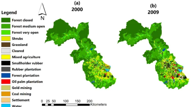
This research used LULC maps of Kutai Barat and Mahakam Ulu for 2000 and 2009. The LULC maps were developed by Budiman, et al. (2014) using an unsupervised classification method (Budiman, Arif, Setiabudi, Hultahera, & Ginanjar, 2014). These 250-meter resolution LULC maps were built based upon Landsat TM/ETM-7 satellite imageries. The overall accuracy of the LULC maps is 89% (van der Laan, 2016). The LULC maps distinguish land cover into 15 classes (Fig. 6). Oil palm and rubber plantations are categorized into three different classes; Smallholder rubber, Rubber plantation and Oil Palm Plantation. However, rubber plantations were treated as a single class during disaggregation processes.
Figure 6. Land used and land cover maps of Kutai Barat and Mahakam Ulu 2000 (a) and 2009 (b) (Budiman, Arif, Setiabudi et al., 2014; van der Laan, 2016)
28 A study conducted by van der Laan (2016) shows that forest degradation and deforestation were mostly caused by large-scale expansion of rubber and oil palm plantations. During 2000 and 2009, about 85,000 ha were converted into oil palm and rubber plantations. In this period, oil palm has increased by about 635% while smallholder rubber and rubber plantation increased by about 85% and 118%, respectively.
3.3 Crop-Specific Biophysical Suitability Map
Food and Agriculture Organization of the United Nations (FAO) and the International Institute for Applied Systems Analysis (IIASA) provide The Global Agro-Ecological Zones (GAEZ) which conveys various global land resources assessments such as land and water resources, agro-climatic resources, suitability and potential yields, downscaled actual yield and production and lastly the yield and production gaps (Food and Agriculture Organization of The United Nations, 2017). FAO has made these datasets available and anyone could access various data through GAEZ data portal web2. Crop-specific biophysical suitability maps were obtained from GAEZ data porta web. Suitability map is built by taking into consideration the soil moisture conditions, radiation, temperature, terrain, pests and water availability.
GAEZ biophysical suitability maps are categorized according to crop type, water supply systems, input level and baseline climate. Water supply systems comprise rainfed, rainfed with water conservation, gravity irrigation, sprinkler irrigation and drip irrigation. However, we focused on using rainfed and gravity irrigation. Input level is distinguished into three categories; low-level inputs, Intermediate level inputs and high-level inputs. According to FAO (2017), the low-level inputs use traditional management assumption where the farming system is subsistence-based, production using traditional cultivars, no application of nutrient and anti-pest treatment. While the intermediate level input uses
2 http://gaez.fao.org/Main.html
29 improved management assumption where the farming system is partly market-oriented (subsistence and commercial sale), production using a combination of labour and mechanization, fertilizer and pest control application. Lastly, the high-level input uses advanced management assumption where farming is mostly market-oriented, production is fully mechanization with low labour, nutrient and pest control application. BPS (2010) shows in Kutai Barat and Mahakam Ulu during 2000 and 2009 number of oil palm and rubber agriculture were dominated by intermediate scale company. Thus, we used suitability map under intermediate level input.
There are 49 types of crops provided by GAEZ. However, rubber is not included in those types of crops. Alternatively, banana suitability map was used to substitute rubber
Figure 7. The intermediate-irrigated oil palm (a), the intermediate-rainfed oil palm (b), and intermediate- rainfed rubber (banana)(c) suitability maps of Kutai Barat and Mahakam Ulu obtained from GAEZ data set (Food and Agriculture Organization of The United Nations, 2017)
30 suitability map. The reason why banana was chosen to substitute rubber suitability map is that intercropping rubber plantation with banana is quite common and popular in numbers of agricultural practices and researches (Boyie Jall, 2009; Rodrigo, Stirling, Silva, & Pathirana, 2005; Rodrigo, Stirling, Teklehaimanot, & Nugawela, 2001). Intercropping is a planting method when a certain type of crop is planted together with the supplementary crop to fill the planting gap. Intercropping is only possible if the intercropped plantations have same or similar suitability factor (Rodrigo et al., 2005). Intercropping is popular partly because its capability to increase farmer productivity by allowing farmers to effectively use the planting spaces. Moreover, in GAEZ data set, the banana suitability map is only available in a rainfed water supply system. Therefore, we used the intermediate rainfed suitability map of rubber as a substitution for the rubber suitability map.
FAO categorized the GAEZ data set based on baseline climate data during a historical period (1961 – 2000) and during future time periods (2020s, 2050s and 2080s). GAEZ data sets are provided in a 5 arc-minutes (± 9 km) spatial resolution. Thus, spatial resampling has to be applied to the GAEZ suitability maps in order to fit the LULC map spatial resolution. The resampled suitability maps of oil palm and rubber (or instead: banana) are depicted in Figure 7. The suitability index is ranging from 0 to 10,000 where the minimum of 0 shows the most unsuitable location and the maximum of 10,000 shows the most suitable location.
3.4 Irrigation Map
Global map or irrigation area developed by the Land and Water Division of the Food and Agriculture Organization of the United Nations and the Rheinische Friedrich-Wilhelms-Universität in Bonn, Germany was used as an irrigation identifier3 (FAO, 2016). The irrigation map has a 5 arc-minutes resolution or about 9 kilometres resolution. Although the resolution is smaller than the LULC map, resampling was unnecessary since the irrigation map was only an identifier whether a certain agriculture area belongs to an
31 irrigated or rainfed area. Irrigated areas are aggregated mostly in southeast and northwest part of the study area (Fig. 8). In the GAEZ data set, suitability map of banana (substitution of rubber) was only available in rainfed water supply system. Thus, the irrigation map was only applied to identify the irrigated and rainfed oil palm plantations. While for the rubber, the rubber plantations in the whole study area were categorized as a rainfed plantation.
3.5 Projected Land Use and Land Cover Map
The 2030 projected land use and land cover maps are simulation results under what-if-policy scenarios. The PCRaster Land Use Change (PLUC) model was utilized to run the simulation and this model was implemented in the PCRaster Python framework (Verstegen, Karssenberg, Van der Hilst, & Faaij, 2012). The PLUC used the numbers of land use types in LULC maps of Kutai Barat and Mahakam Ulu from 1990, 2000, and 2009 as a function of a set of user-specified spatio-temporal suitability factors and a no-go area for each land use type. The simulation model takes two factors into consideration; projected
32 land allocation zoning policies and projected land use demand development. Land allocation zoning scenarios consist of restricted and unrestricted scenarios. Restricted zoning scenario assumes that agriculture and mining expansion is restricted to non-forest and non-peatland area. While unrestricted zoning scenario allows agriculture and mining to occur in forest and peatland area except for protected forest zone (van der Laan, 2016).
Table 4. Actual land use and land cover in 1990, 2000, 2009 and projected LULC in 2030 of Kutai Barat and Mahakam Ulu
1990 2000 2009 Limited restricted Limited unrestricted Unlimited restricted Unlimited unrestricted Mixed agriculture 11,600 15,600 26,200 32,431 32,431 43,494 64,863 Smallholder rubber 44,000 66,100 122,500 Rubber plantation 1,000 1,400 3,000 Forest plantation 8,100 16,400 31,700 44,900 44,900 139,469 105,675 Oil palm plantation 100 4,200 31,200 115,225 115,225 328,900 1,466,425 Gold mining 100 600 100
Coal mining 600 800 7,800
Settlement 3,100 3,200 6,700 8,425 8,425 8,594 10,081 Projected LULC in 2030 (ha)
166,975 167,100 Land use type
Actual Area (ha)
15,888 15,881 150,600 156,788 332,781 217,413
The land use demand development defines two dimensions of development; limited and unlimited development. The limited development implements the presidential instruction no 6 year 2013 regarding the limitation of mining, pulpwood and oil palm plantation permit on forested land and peat land (Republik Indonesia, 2013a). Under the limited scenario, the land development will follow exponential curve until 2014 and after that, the demand will decrease 50% annually resulting a s-shaped curve. On the other hand, the unlimited development will follow the extrapolated exponential trend of the land use development from 1990 to 2009 with the maximum land area available as a threshold (van der Laan, 2016). According to these dimensions of development, we had four projected LULC scenarios of Kutai Barat and Mahakam Ulu in 2030. Later, least square regression was performed over these scenarios in order to estimate the oil palm and rubber yield in 2030.
Figure 9. depicts the projected LULC of Kutai Barat and Mahakam Ulu in 2030 under four scenarios. Roughly, we see substantial development differences between the restricted and the unrestricted scenarios. The unrestricted scenario is prone to allow greater expansion
33 than the restricted scenario, particularly for oil palm plantation. Detail area for each land use type from 1990 to 2009 as well as projected LULC in 2030 is conveyed in Table 4.
4 RESULTS AND DISCUSSIONS
As described in section 2.3, the first step of SPAM disaggregation process is the determination of the suitability index on each pixel of oil palm and rubber land use. The suitability indexes of oil palm and rubber in 2000 and 2009 are depicted by the suitability maps in Figure 10. In the rubber suitability map for the whole study area (Fig. 10a), we might see the blocky pattern in the south-east part of the study area. This pattern represents the irrigated suitability indexes of oil palm. Visually the irrigated suitability indexes are prone to have a lower value than the rainfed area.
Figure 9. The projected LULC maps of Kutai Barat and Mahakam Ulu in 2030 as result of the PLUC simulation model under the four allocation zoning policies and land use demand development scenarios
34 The disaggregated oil palm and rubber yields are depicted in Figure 11. We see that oil palm and rubber have expanded from 2000 to 2009. The rubber plantations are concentrated in the south-east part of the study area and are expanding radially in every direction. Moreover, if we refer to rubber disaggregated yield, the rubber expansion is followed by the increase of the average yield from 0.14 to 1.25 ton/ha while the oil palm expansion in 2009 is followed by the degradation of the average yield from 4.50 to 1.86 ton CPO/ha (Tab. 5). At glance, it may show a degradation of the oil palm yield, but if we considered the cropping period of oil palm, it takes averagely three to four years for the oil palm plantation to be able to be harvested and reach its peak production (Food and Agriculture Organization of The United Nations, 1997). Thus, we presume that the oil plantations were in early harvesting stage in 2009.
Figure 10. Modified suitability maps of oil palm and rubber for whole area of Kutai Barat and Mahakam Ulu (a), based on the LULC map in 2000 (b) and 2009 (c), water supply systems (irrigated/rainfed), input level (intermediate), and crop types (oil palm/rubber)
35 Referring to Kutai Barat and Mahakam Ulu crop statistics data in 2000 and 2009 (Badan Pusat Statistik Provinsi Kalimantan Timur, 2001, 2010), the average yields of oil palm is 2.14 ton CPO/ha in 2000 and 4.72 ton CPO/ha while average yields of rubber is 0.32 ton/ha in 2000 and 0.85 ton/ha in 2009. The national yield of oil palm and rubber are conveyed in Table 5. The average disaggregated oil palm yield exhibits substantial high value particularly in 2000 (4.50 ton CPO/ha) when the national yield is 1.68 ton CPO/ha and the Kutai Barat and Mahakam Ulu yield is 2.14 ton CPO/ha. On the other hand, the average disaggregated rubber yield exhibits lower yields compared to national and Kutai Barat and Mahakam ulu yield in both year. These differences occur due to the different cropping area reported in crop statistics data and the cropping area identified from the LULC maps (Fig. 18). The area differences are quite large, consequently the average yield become different as well.
Figure 11. The disaggregated oil palm (a,b) and rubber (c,d) yields of Kutai Barat and Mahakam Ulu in 2000 and 2009 as results of the SPAM disaggregation method implementation
36
Table 5. Comparison between national, Kutai Barat and Mahakam Ulu and the disaggregated yield of oil palm and rubber in 2000 and 2009 ((Badan Pusat Statistik Provinsi Kalimantan Timur, 2001, 2010; Kementerian Pertanian, 2016)
Crop Yield Oil palm production ton CPO/ha)
Rubber production (ton/ha) 2000 2009 2000 2009 National 1.68 2.45 0.45 0.71 Kutai Barat 2.14 0.71 0.32 0.85 SPAM 4.5 1.86 0.14 0.25
Figure 12 shows the hot-spot distributions of oil palm and rubber yields in 2000 and 2009. The high yields (hot-spot) as well as the low yields (cold-spot) of oil palm yields in 2000 and 2009 do not show any particular aggregation patterns, but instead the distributions are prone to be dispersed. Moreover, the cold-spots occur most likely in the irrigated area. This result is expected since oil palm plantations particularly in tropical area (e.g. Indonesia and Malaysia) are predominantly use rainfed system as water use supply. Oil palm plantations are able to produce higher in a rainfed environment than in an irrigated environment (Ludwig et al., 2011). Compared to other crop such as wheat and rice, oil palm plantation is able to reach its peak production with only relying on rainfed water supply.
While for the rubber yields, the hot-spots are aggregated in the south-east part and the cold-spots are aggregated in the north part of the study area. Moreover, sub-district crop statistic data shows that sub-district such as Bentian Besar, Jempang and Bongan that have the relatively high yield are located in the south-east part of Kutai Barat and Mahakam Ulu. The north part of the study area is predominately a forested land. Thus, we presumed that the south-eastern part of Kutai Barat and Mahakam Ulu are able to provide a higher yield than the northern part. If the rubber plantation expanded towards the north forested land, the rubber yields tend to be lower than if the rubber expanded towards the south-east direction.
37 According to BPS (2001 & 2010), Kutai Barat and Mahakam Ulu have the largest rubber plantation area as well as the biggest rubber production among other districts in East Kalimantan either in 2000 or 2009 (Tab.3). Rubber plantation has expanded about 19.03% while oil palm plantation has expanded about 39.62% during 2000 and 2009. Oil palm exhibits a larger expansion rate than rubber and is prone to expand even further in the future. According to the projected LULC scenarios of Kutai Barat and Mahakam Ulu in 2030, the oil palm cropping areas have potentially expanded with about 369 – 4700% while rubber cropping areas are potentially expanded about 133 – 265%. Considering this potential expansion, we further analyzed the potential benefit given by this expansion by assessing the yields of oil palm and rubber plantations. Based on our finding, during 2000 and 2009, low yields are prone to occur in the irrigated area and toward the north forest land. In order to improve the oil palm and rubber yields, the cropping area should use the rainfed water supply system and the expansions are suggested to explore the south-eastern part of Kutai Barat and Mahakam Ulu.
Figure 12. Hot spot distribution of oil palm (a,b) and rubber (c,d) yields of Kutai Barat and Mahakam Ulu in 2000 and 2009
38 In order to justify whether the oil palm plantation in 2009 was in early harvesting stage or it was really a degradation of the oil palm yield, we compared the original SPAM disaggregation result with the maintained yield method result (Fig. 13). If we look at the disaggregation results between these two methods, we might not be able to see much differences. However, according to the density histograms of the original SPAM and maintained yield results (see Figure A1 in appendix), the yield distributions in maintained yield method are concentrated in the low and high value. Since the maintained yield method forces the yield value at the overlapped pixel in 2009 to be equal with the yield value in 2000, the yield distributions are pushed away from the overlapped yield values. For example, the overlapped rubber yields are ranging from approximately 200 – 250 kg/ha, then on the maintained rubber yield distributions, the rubber yield values below 200 and above 250 increase. While for the oil palm, the overlapped oil palm yields are ranging from approximately 5000 – 6600 kg CPO/ha, since the oil palm yield in 2009 are mostly lower
Figure 13. The original SPAM disaggregation (a) and the maintained yield method results of oil palm and rubber yields in 2009.