Master of Science in Viticulture & Enology
Joint diploma “EuroMaster Vinifera” awarded by:
INSTITUT NATIONAL D'ETUDES SUPERIEURES AGRONOMIQUES DE MONTPELLIER AND
INSTITUTO SUPERIOR DE AGRONOMIA DA UNIVERSIDADE DE LISBOA
Master thesis
Basal leaf removal to reduce fruitset and induce smaller and looser clusters in
variety Trincadeira with compact bunches
Lorenza BAZZANO 2014-2016
Supervisor : Professor Carlos Manuel Antunes LOPES, ISA University of Lisbon Supervisor : Professor Vittorino NOVELLO, University of Turin – DISAFA
Jury:
President- Professor Jorge Manuel Rodrigues Ricardo da Silva, ISA, University of Lisbon. Members- Professor Vittorino Novello, University of Turin – DISAFA;
Auxiliary Professor Ricardo Nuno da Fonseca Garcia Pereira Braga, ISA, University of Lisbon; Auxiliary Researcher José Manuel Couto Silvestre, INIA, I.P. – Dois Portos.
I
Acknowledgment
In first place, my thanks go to Professor Carlos Manuel Antunes Lopes for giving me the opportunity of working in this project and for the inestimable help during the writing of my Master Thesis. I sincerely thank Ricardo Egipto, João Graça, Tobias Winkler, Gonçalo Victorino and Helena Horvat for their priceless help: this work would not have been accomplished without it.
To my adored family, to all my friends and my Master colleagues, thanks for giving me the ambition, the strength, the understanding and the inspiration which guided me throughout my journey in this Master.
In conclusion, my gratitude goes to Vinifera EuroMaster, without which nothing of this would have been possible.
II
Table of contents
Acknowledgment ... I Table of contents ... II List of Figures ... IV List of Tables ... VII List of Equations ... VII List of Abbreviations... VIII Abstract ... IX Resumo ... X 1 Introduction ... 1 1.1. Introduction... 1 1.2. Objectives ... 2 2 Literature review ... 3
2.1. Viticulture in the World and Portugal ... 3
2.2. Vitis Vinifera L. cv Trincadeira: Compact Bunches and Linked Disadvantages ... 3
Bunch Compactness Evaluation ... 5
2.3. Basal Leaf Removal ... 7
2.4. Carbohydrates and their importance ... 7
2.5. Grapevine Canopy and Leaf Area ... 9
Canopy Management Effects ... 10
2.6. Light Microclimate ... 11
Effects of Defoliation on Sunlight Interception ... 12
2.7. Grapevine Fruitfulness: Flowering and Fruitset ... 13
2.8. Grape Composition and Wine Quality ... 15
3 Materials & Methods ... 17
3.1. Site Description ... 17
3.1.1. Site Management ... 18
3.1.2. Experimental Design ... 18
III
3.2.1. Phenological development ... 19
3.2.2. Leaf Area ... 19
3.2.1. Fruitfulness ... 20
3.2.2. Cluster Light Microclimate ... 22
3.2.3. Leaf Layer number and Canopy Dimensions ... 22
3.2.4. Stem Water Potential ... 23
3.2.5. Laboratory Analysis on Grape Composition ... 23
- pH ... 23
- TA ... 23
- °Brix & Potential Alcohol... 24
- Anthocyanins ... 24
- Total Phenols ... 24
3.2.6. Harvest Protocol ... 24
3.2.7. Data Analysis ... 25
4 Results and Discussions ... 26
4.1. Meteorological Data ... 26
4.1.1. Weather in 2016 ... 26
4.1.2. Light Incidence ... 28
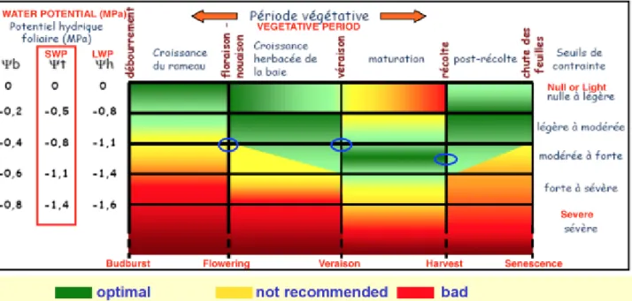
4.1.3. Stem Water Potential ... 30
4.2. Vegetative Growth ... 32
4.2.1. Phenological Development ... 32
4.2.2. Canopy dimension and Point Quadrat Assessment ... 33
4.2.3. Leaf Area ... 36
Primary Leaf Area ... 36
Lateral Leaf Area ... 37
Total Leaf Area ... 37
4.3. Reproductive cycle ... 39
4.3.1. Fruitset ... 39
4.3.2. Yield, Vigor and Bunch compactness ... 41
4.4. Grape Composition and Quality ... 44
5 Conclusions... 46
IV
List of Figures
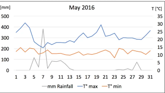
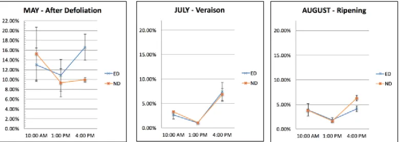
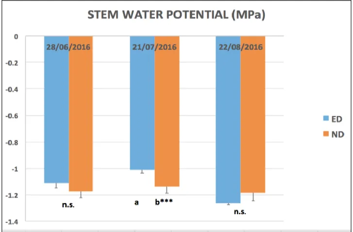
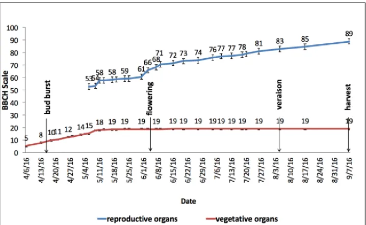
Figure 1: Aerial Picture of Tapada da Ajuda Vineyard, in Instituto Superior de Agronomia, Lisboa. The red circle indicates the Vinha do Almotivo (source: Google Maps). ... 17 Figure 2: Counting of the flowers from the inflorescence with Image Analysis: picture on the left shows the counting on the entire inflorescence; picture on the right shows the counting of the flower of the same inflorescence, after separation. ... 20 Figure 3: Linear regression between the number of flowers counted on the entire flower as a predictor (x), and the number of flower counted after separating as a dependent variable or predicted (y). ... 21 Figure 4: Selected cluster photographed at harvest: in the left picture, the entire cluster; in the central picture, the berries of the same cluster, after separation; in the picture on the right, counting the berries with Image Analysis. ... 21 Figure 5: Temperatures (°C) in Lisbon during 2016 year. Red line showing the maximum T°, green line showing the average T°, blue line showing the minimum T°. Data from Instituto Superior Tecnico, Lisbon. ... 26 Figure 6: Precipitation (mm) in Lisbon during 2016 year. Data from Instituto Superior Tecnico, Lisbon. ... 26 Figure 7: Precipitation (mm) and temperatures (°C) in Lisbon during the month of May 2016. Data from Tapada da Ajuda, Lisbon. ... 27 Figure 8: % PAR measurements with ceptometer during flowering (May), veraison (July) and ripening (August); in defoliated (ED) rows and non-defoliated (ND) ones. ... 28 Figure 9: Midday stem water potential measured in Trincadeira vineyard, Tapada da Ajuda, during three different phenological stages: post-flowering (28th June), veraison (21st July) and ripening (22nd August); in early defoliated (ED) and non-defoliated (ND) rows. ... 30 Figure 10: Values of water potential along the vegetative period; in green indicated optimal range of water deficit for a high quality red wine; blue circles show the measured SWP in Trincadeira vineyard. Adapted from Ojeda, 2007. ... 31 Figure 11: Phenological development during 2016 vegetative season of cv Trincadeira, in Tapada da Ajuda, Lisboa. ... 32
V
Figure 12: On the top, graph showing the canopy height and width, expressed in meters, in defoliated (D) and non-defoliated (ND) rows; at the bottom, the exposed leaf area obtained
with Equation 1 and expressed in m2/ha, in defoliated and non-defoliated rows. ... 33
Figure 13: On the top, the Leaf Layer Number determined in defoliated(D) and non-defoliated (ND) rows; at the bottom, the % of leaves inside the canopy and the % of clusters uncovered by the canopy, both in defoliated and non-defoliated rows. ... 34
Figure 14: Trincadeira vines in Non-Defoliated rows; in the left picture, the entire canopy, cluster zone in the central picture, single cluster in the picture on the right. ... 35
Figure 15: Trincadeira vines in Defoliated rows; in the left picture, the entire canopy, cluster zone in the central picture, single cluster in the picture on the right. ... 35
Figure 16: Primary Shoot Leaf Area in m2 for treatments defoliated (D) and non-defoliated (ND) and for the following assessments: May, before defoliation; May Def = after defoliation; June BT =before shoot trimming; June AT = after Shoot trimming; July and August; n.s. = no significant differences between treatments, * = significance level 0.1, **= significance level 0.05, *** = significance level 0.01. ... 36
Figure 17: Lateral Shoot Leaf Area in m2 for treatments defoliated (D) and non-defoliated (ND) and for the following assessments: May, before defoliation; May Def = after defoliation; June BT =before shoot trimming; June AT = after Shoot trimming; July and August; n.s. = no significant differences between treatments, * = significance level 0.1, **= significance level 0.05, *** = significance level 0.01. ... 37
Figure 18: : Total Shoot Leaf Area in m2 for treatments defoliated (D) and non-defoliated (ND)F and for the following assessments: May, before defoliation; May Def = after defoliation; June BT =before shoot trimming; June AT = after Shoot trimming; July and August; n.s. = no significant differences between treatments, * = significance level 0.1, **= significance level 0.05, *** = significance level 0.01 ... 38
Figure 19: Percentage of fruitset in early-defoliated (ED) and non-defoliated (ND) treatment. ... 39
Figure 20: Photos of cluster with abnormal fruitset, along the season. ... 40
Figure 21: Bunches with different compactness, pictures taken in field conditions. ... 42 Figure 22: Different compactness in bunches from the same vines. Two photos on the top show two selected bunches from vine number 4 in row 13 (Early Defoliated treatment); two photos on
VI
the bottom show two selected bunches from vine number 24 in row 14 (Non-Defoliated treatment). ... 43 Figure 23: Grape quality components, assessed at pre-veraison (25th July), post-veraison (8th
August), ripening (22nd August) and harvest (5th September); in early-defoliated (ED) and non-defoliated (ND) treatments... 45
VII
List of Tables
Table 1: Criteria for bunch compactness evaluation. Adapted from Tello (2014). ... 6 Table 2: Yield and yield components, comparison of early-defoliated (ED) and non-defoliated (ND) treatment. From left to right: the average percentage of fruitset, the yield calculated as kg of grapes per vine, the total number of bunches per vine, the average bunch weight of the selected clusters, index of bunch compactness in average, and the ratio between leaf area per vine and yield per vine. ... 41
List of Equations
PLA = 0.9619238 ∗ MLA11.01515 Equation 1 19
LLA = 1.027245 ∗ MLA20.97829 Equation 2 19
y = 2.4116x + 0.1252 Equation 3 21
VIII
List of Abbreviations
, psi Water Potential
BL Basal Leaf
BLR Basal Leaf Removal
ED Early Defoliation Treatment
LA Leaf Area
LAI Leaf Area Index
LLN LLA
Leaf Layer Number Lateral Leaf Area
ND Control Non-Defoliated
PAR PLA
Photosynthetically Active Radiation Primary Leaf Area
SA External Leaf Area
PA PPFD TLA
Potential Alcohol
Photosynthetic Photon Flux Density Total Leaf Area
IX
Abstract
This paper studies whether pre-flowering basal leaf removal is able to modify the cluster compactness in Vitis vinifera L. cv Trincadeira, as well as its berry composition and canopy density, in order to avoid the incidence of diseases such as Botrytis bunch rot.
The first six leaves were removed for an early defoliation treatment (ED) performed at pre-bloom, and this was compared with a control non-defoliated (ND). During the vegetative season, various analyses were performed: monitoring phenology development, leaf area measurements, radiations analysis, stem water potential, canopy dimensions and Point Quadrat assessments, fruitfulness, bunch compactness estimation and berry composition.
Results seem to point out that early defoliated vines went through a prompt recovery, with a great lateral shoots and leaves regrowth.
Despite no significant difference was proven in the analyses from the two treatments, leaf area and canopy dimension appears to be greater in ND vines all along the season up until ripening, when ED vines show higher values. Clusters affected by coulure and millerandage were found both in ED and in ND vines, demonstrating that fruitset was not optimal in the whole plot.
Trincadeira’s high vigor and unsuitable environment conditions during 2016 season were found to have a greater impact than expected.
Significance of the study: The goal is to provide viticulturists with tools to optimize the wine grape
production, using a feasible field operation.
KEY WORDS: early basal leaf removal; bunch compactness; Trincadeira; leaf area; shoot vigor;
X
Resumo
O objetivo desta dissertação é estudar o efeito da desfolha basal à pré-floração (pré-desfolha) na compacticidade dos cachos na casta Trincadeira, assim como na composição dos bagos e densidade da sebe, de modo a prevenir a incidência de doenças como a podridão cinzenta (Botrytis cinerea). As primeiras 6 folhas da zona basal da sebe foram removidas antes da floração, num conjunto de videiras. As videiras que sofreram esta pré-desfolha foram comparadas com videiras não desfolhadas (controlo). Durante o desenvolvimento vegetativo foram feitas várias análises: monitorização do desenvolvimento fenológico, medições de área foliar, análise da radiação incidida, potencial hídrico de stem, dimensões da sebe e avaliações Point Quadrat, fertilidade, estimativa da compactidade dos cachos e composição dos bagos.
Os resultados indicam que as videiras sujeitas à pré-desfolha recuperaram a sua área foliar com um rápido desenvolvimento de sarmentos e folhas netas.
Apesar de não terem sido encontradas diferenças significativas entre os dois métodos, a área foliar e a dimensão da sebe aparentam ser superiores em videiras não desfolhadas durante todo o ciclo da videira com exceção à época da vindima, altura em que as videiras pré-desfolhadas apresentam valores superiores. Foram encontrados cachos afetados por desavinho e bagoinha em ambos os métodos de desfolha, o que indica que o vingamento não foi ótimo em toda a parcela.
O elevado vigor da casta Trincadeira e as condições climatéricas impróprias durante a campanha 2016 tiveram um impacto superior ao esperado.
Relevância do estudo: O presente estudo pretende proporcionar aos viticultores ferramentas que
1
1 Introduction
1.1.
Introduction
Basal leaf removal is among the viticultural practices which is increasingly recognized as an important tool to manipulate grapevine, both in terms of production and quality.
Performed in the cluster zone, usually in the time frame from fruit-set to veraison, basal leaf removal is used by viticulturists to increase porosity in dense canopies, improving aeration and bunch exposure to light, with the aim to improve the berry color, the bunch resistance to rot and the ripening of grapes.
Being the basal leaves the oldest and the typical source organ producing photosynthates, when they are removed before flowering the total carbohydrates availability is weakened. Thus, flowers can fail to open and some of the inflorescences may be lost. These effects are investigated as a way to regulate the yield by decreasing the fruitset.
Early basal leaf removal is shown to result in smaller berries and looser clusters. The latter has a particular beneficial effect in reducing the risk of rot incidence, such as Botrytis, while small berries are favored in quality wine production, because of a higher skin-to-pulp ratio, contributing to more intense color and aromas in wines. Moreover, an improved canopy microclimate, facilitating clusters exposure, is found to lead to lower level of organic acid, to have an impact on sugar content of grapes, and to strongly influence the total phenols in berry composition.
Ultimately, open canopies are shown to achieve high quality wine, well structured, with more ripen notes and suitable for ageing.
Hence, if defoliation was traditionally not performed around blooming to prevent negative effects and a decrease in yields, recently its performance has been investigated to promote a better canopy microclimate and berry composition in high-yielding and vigorous grapevine varieties.
This work has been performed on the cultivar Trincadeira, a Portuguese grapevine variety characterized by high vigor and susceptibility to bunch rot, giving rise to the necessity for a canopy management favoring air circulation.
2
1.2.
Objectives
The aim of the present research is to investigate the effects of basal leaf removal performed at pre-flowering on cv Trincadeira, in Lisboa region. The influence of this viticultural practice has been examined on yield components, on canopy microclimate, on the canopy dimension response and on the effects on fruit composition and sanitary status.
This will allow viticulturists to be aware of an easy way to manage the vine microclimate, so to take deliberate decisions in order to obtain the most advantageous canopy.
3
2 Literature review
2.1.
Viticulture in the World and Portugal
Grapevine has been among the first fruit species to be domesticated and nowadays it is the world’s most economically important fruit crop (Keller, 2010).
Grapes are cultivated in six out of seven continents, between latitudes 4° and 51° in the Northern Hemisphere and between 6° and 45° in the Southern Hemisphere, across climates of great diversification (oceanic, warm oceanic, transition temperate, continental, cold continental, Mediterranean, subtropical, attenuated tropical, arid and hyper arid climates) (Schultz and Stoll, 2010). The most important areas for grape production are located between latitudes around 30° and 50° in the Northern Hemisphere and between latitudes around about 30° and 40° in the Southern Hemisphere, which correspond to regions with a temperate climate, where the mean temperature of the warmest month is superior to 18°C and the mean temperature of the coldest month goes over -1ºC (Reisch et al., 2012).
As grapes (Vitis spp.) are world widely so important, their global production reached around 73.7 million tons in 2014 (OIV, 2015). Undoubtedly, winemaking is the most important use of grapes, both in terms of amount and area, leading to a production of 270 millions of hectoliters in 2014 (OIV, 2015).
The European countries touching the Mediterranean Sea, where grapes have been cultivated for thousands of years, are dominant grape growers and wine producers. Among these, Portugal stands with 224 thousands of hectares under vines, with a wine production of 6.2 millions of hectoliters in 2014, positioning itself as the 11th largest world producer of wine (OIV, 2015). One peculiarity of Portugal is that there are 340 cultivars officially authorized for wine making (Veloso, 2008). One of this cultivated varieties has been used in this experimentation: Trincadeira, typical from Alentejo region, the second biggest region in Portugal for wine production, after Douro e Porto (Veloso, 2008).
2.2.
Vitis Vinifera L. cv Trincadeira: Compact Bunches and Linked
Disadvantages
Trincadeira is a very important Portuguese grapevine cultivar, which can make red wines characterized by raspberry fruit, spicy notes, peppery, herbal flavors, and very fresh acidity. This
4
grape grows all over Portugal, but it is at its best in dry and warm areas, such as Alentejo. Nevertheless, it is grown also in Douro, where it is known as Tinta Amarela (Eiras-Dias et al., 2011). Although giving rise to unique and excellent wines, it presents extremely irregular berry ripening among seasons, probably due to high susceptibility to abiotic and biotic stresses (Fortes et al., 2011), and appears to be remarkably susceptible to fungal pathogens such as grey mold, caused by Botrytis cinerea, which is one of the most dramatic grape diseases (Agudelo-Romero et al., 2014).
Grapevines are prone to several diseases, with fungi being the major cause of damage and losses in grape quality and yields, consequently affecting wine production worldwide (Agudelo-Romero et al., 2014). The presence in grapevines of Botrytis cinerea, a necrotrophic fungus commonly known as Botrytis bunch rot and/or grey mold, causes severe reductions in both quality and quantity of grapes and wine as a consequence of modifications in the chemical composition of the grape berry itself (Bocquet and Valade, 1995). Grey mold outbreaks can be very heterogeneous in space and time, and bunches can be partly or totally damaged, affecting crop yield and fruit quality (Cadle-Davidson, 2008; Coertze and Holz, 2002). In fact, beside the direct loss of yield and quality of grapes, it can worsen the quality of wines by generating off-flavors, oxidative damage, premature aging and difficulties in clarification during the winemaking process (Ribéreau-Gayon et al., 2006). The epidemiology of this disease in the vineyard is supposed to have numerous causes, such as climatic factors, vine vegetative and reproductive vigor (Valdés-Gómez et al., 2008), and genetically-determined morphological and biochemical features of the berry (Commenil et al., 1997; Deytieux-Belleau et al., 2009; Gabler et al. 2003; Goetz et al., 1999).
For the variety Trincadeira, one of the main causes of the susceptibility to mold is linked to the compactness of its bunches (Eiras-Dias et al., 2011).
As a matter of fact, bunch compactness in grapevine is an important trait affecting the sanitary status and so the quality of grapes (Tello and Ibáñez, 2014). Bunch compactness is described as the degree of compaction of the berries along the rachis. It results from the arrangement of the solid components (berries) in the three-dimensional volume of the bunch, which is determined by the architecture of the rachis. Berries are sparsely distributed in loose bunches, whereas they are densely packed in the compact ones (Tello and Ibáñez, 2014).
The dense distribution of the berries in compact bunches has an impact on the fruit quality from many perspectives: the aeration of the bunch is compromised, as well as the exposure of individual
5
berries to sun radiation (Vail and Marois, 1991). Indeed, in compact bunches the microclimate is more favorable for the development of different organisms, due to the high humidity caused by delay of berry drying after rain events and water retention (Vail and Marois, 1991; Vail et al., 1998). Moreover, higher pressure caused by the neighbor berries during their growth may lead to cracks in the berries skin (Becker and Knoche, 2012; Molitor et al., 2012). This can be reinforced by the fact that the close contact of berries in compact bunches may modify the biochemical composition and thickness of berry skin (Gabler et al., 2003). In fact, the regular formation of epicuticular waxes may be impeded in the areas where berries are in close contact (Becker and Knoche, 2012; Commenil et al., 1997; Gabler et al., 2003; Marois et al., 1986). So, when the berry skins come to cracking, the out coming water and nutrients will facilitate conidia germination and mold development (Marois et al., 1986), which is a proper outset for fungal epidemics (Molitor et al., 2012).
Eventually, all of these elements show the reason why B. cinerea epidemiology grapevine is recognized as one of the major issues for grapevine with compact bunches (Alonso-Villaverde et al., 2008; Hed et al., 2009; Vail and Marois 1991; Vail et al., 1998).
Beside the development of pests and diseases, another noticeable aspect related to bunch compactness concern the berries ripeness. In compact bunches there are a greater number of inner berries (Vail and Marois, 1991) which will receive a lower solar radiation intake, compared to the more exposed ones. This will lead to a heterogeneous ripening along the bunch and in the vineyard, making the harvest date decision more complex.
Bunch Compactness Evaluation
Grapevine bunch compactness can be categorized from loose to dense (Cubero et al., 2015). In dense bunches, berries are stuffed and touching each other, and in case of great compaction they can lose their rounded shape. Also, part of the berries can be hidden inside the cluster, where air circulation and sun exposure are compromised (Vail and Marois, 1991; Molitor et al., 2012).
Grapevine bunch compactness can be evaluated in multiple ways. The quicker and easier method is a visual assessment.
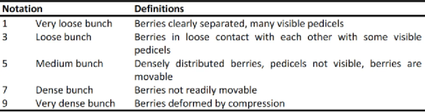
The descriptor code 204 of the International Organization of Vine and Wine (OIV, 2009) describes the criteria for this evaluation, implicating an examination of the biggest clusters in ten different shoots, and a classification into five different classes (1, 3, 5, 7, 9), taking into consideration the
6
density of berry distribution, their mobility and deformation and the exposure of the pedicels (OIV, 2007) (Table 1).
Table 1: Criteria for bunch compactness evaluation. Adapted from Tello (2014).
This OIV method is largely used in the grape and wine sector, but it depends on the evaluator’s judgement and experience. The results are thus susceptible to a considerable variability (Cubero et al., 2015).
Visual methods, even though their simplicity, are subjective and hence unfeasible for objective measurements (Tello and Ibáñez, 2014). To overcome the inaccuracy of visual assessments, other authors have provided methods for bunch compactness estimation based on the relation between different parts of the cluster. One of the most common is the value obtained from the ratio between the total berry number and the length of the rachis (Vail and Marois, 1991; Palliotti et al., 2011, Palliotti et al., 2012; Tello and Ibáñez 2014; Cubero et al., 2015). Similarly, other methods propose the ratio between the bunch weight and its length (Sternad-Lemut et al., 2015), or the number of berries per the length of different parts of the rachis (Dokoozlian and Peacock, 2001; Intrieri et al., 2013).
In response to the importance of the grape sanitary status for the market, numerous strategies to lessen bunch compactness have been investigated. Two different approaches are distinguishable: one is based on the application of different agrochemicals to the vines - for example with the use of growth regulators; the other one includes strategies to adjust the source-to-sink ratio of the vine, in order to promote a source limitation and so to loosen the bunches be a lower fruitset. The latter include the removal of different vegetative organs of the plant.
7
2.3.
Basal Leaf Removal
Basal leaf removal, therefore in fruit-zone, is one of the most commonly applied canopy management operations in viticulture, whether manual or mechanical (Reynolds et al., 1996). The influence of timing and method of basal defoliation has been investigated by various authors (Poni et al., 2006; Intrieri et al., 2008; Matus et al., 2009; Sabbatini et al., 2010; Tardaguila et al., 2010; Diago et al., 2012; Gatti et al., 2012; Palliotti et al., 2012; Poni et al., 2013;).
Traditionally performed from fruit-set to veraison, basal leaf removal alters the microclimate of the fruit-zone and it can be performed with different goals: to improve porosity in dense canopy varieties, to ameliorate light exposure and air circulation, to bring advantages in terms of berry color and rot resistance (Bledsoe et al., 1988; Reynolds et al., 1996), as well as berry ripening (Percival et al., 1994).
Recently, an increased attention has been paid to the use of this operation during an earlier phenological stage: before flowering, corresponding to the stage 57 of the BBCH scale (Lorenz et al., 1995).
Pre-flowering basal leaf removal has been investigated to examine its influence on yield components (Poni et al., 2006), on canopy microclimate improvement (Tardaguila et al., 2010), on the effects brought on fruit and wine compositions (Diago et al., 2010; Tardaguila et al., 2010), and also to explore the existing relationship between yield and availability of carbohydrates before blooming (Caspari et al., 1998).
2.4.
Carbohydrates and their importance
In all plants, including grapevine, energy is obtained through photosynthesis, a process by which sunlight is converted into chemical energy, used to synthetize organic compounds (glucose) from inorganic compounds (CO2 and H2O) acquired from the external atmosphere (Keller, 2010).
These resulting compounds, sugars or rather carbohydrates, are the energy suppliers playing a major role in the plant development (May, 2004; Keller, 2010).
The main utilization of the carbon fixed during photosynthesis is its consumption during the respiration process, as it generates ATP (adenosine triphosphate, a coenzyme used for energy transfer), or it is used as “building blocks” for the assemblage of other compounds (such as amino acids) necessary for the metabolism and the cell growth (Keller, 2010).
8
Another crucial role of carbohydrates is in the storage process, where it is converted into starch, the principal reserve of plants (Keller, 2010).
In viticulture, the supply of carbohydrates dispensed to the fruit determines the yields (Keller, 2010). From budburst until complete flowering, the growth of inflorescences is in competition with the fast growth of the young shoots (May, 2004). During the beginning of the season, carbohydrates and nitrogen compounds, the metabolites necessary for the growth gathered during the previous season, are wholly extracted from the overwintering reserves in the trunk and other perennial organs of the vine. Taking into consideration that a leaf reaches maturity roughly 40 days after unfolding (Keller, 2010), the newly assimilated metabolites become of major importance only after the first leaves reach half of their final size (May, 2004; Diago et al., 2012).
From this stage, the metabolites are mainly relocated into the shoot apex, which is a more powerful sink compared to the inflorescences (Fregoni, 1998). Thus, if removing the shoot tip during flowering can improve fruit-set, a basal leaf removal (BLR) is suggested to have an opposite effect: it induces the inflorescences to develop normally until flowering, but afterwards flowers can fail to open, and some of the inflorescences may be lost (May, 2004). This happens because the total carbohydrates availability is weakened when basal leaves are removed (Diago et al. 2012), as mature leaves are the typical source organ producing photosynthates (Keller, 2010).
In fact, the basal and oldest leaves naturally start to transport assimilates to other organs only when the shoot reaches 5 to 6 leaves (Keller, 2010). This transport is addressed to the shoot tip as long as the next leaf above turns from sink to source as well. Then, the assimilates movement from the oldest leaf is redirected towards the shoot base and to other organs of the vine (Keller, 2010), such as inflorescences (Fregoni, 1998).
In various researches, it was indeed shown that yield can be regulated by a decrease in fruit-set, having smaller and looser clusters, obtained with BLR at pre-bloom (Poni et al. 2006, Intrieri et al. 2008, Tardaguila et al. 2010).
However, when BL are missing, the flower itself needs to import carbohydrates from elsewhere to support its development (May, 2004).
Indeed, the restriction in the carbohydrates supply caused by BLR was found effectively compensated by the vine through increased lateral shoots growth. Moreover, the compensatory leaf recovery of the plant was also reported to lead to a “younger” canopy, photosynthetically more
9
active (Candolfi-Vasconcelos, 1991; Palliotti et al., 2000; Hunter, 2000; Petrie et al. 2000; Diago et al., 2012; Intrieri et al., 2008).
2.5.
Grapevine Canopy and Leaf Area
Vine canopy is described by the leaves and shoots system of the plant. It is characterized by its extent in terms of space: width, height and length. But also, by its load of shoots and leaves within its volume, usually accounted as leaf area (Smart et al., 1990). Leaf area (LA) is the one-sided area of a leaf lamina, and it can be calculated for a single leaf (Carbonneau, 1976; Lopes and Pinto, 2000) as well as for a single shoot (Carbonneau, 1976; Barbagallo et al., 1996; Lopes et al., 2005), a single plant or per square meter ground as Leaf Area Index (LAI) (Watson, 1947).
Kliewer and Dokoozlian (2005) define LA as a basic indicator to determine the vine balance and the fruiting capacity of the plant. LA characterizes the canopy density: a crowded canopy is where there is much leaf area within its volume (Smart et al., 1990).
An excessive LA is synonymous of high vigor, while a not sufficient LA may reduce the vineyard production (Champagnol, 1984). To calculate the canopy density, it is possible to use the ratio of LA per canopy surface area or per leaf layer number (LLN) (Smart et al., 1990).
Grapevine growth starts without any leaves and ends with a large canopy (Siegfried et al., 2007).
Being the vine a deciduous plant, the leaf area follows a yearly growth model comparable to the one followed by the shoots: when the vegetative cycle starts, the shoot germinates from an axillary bud formed in the prior season, which already enclose a definite number of nodes, inter-nodes and inflorescence primordia (Sánchez-de-Miguel et al., 2010).
The final leaf area development appears to be influenced by water availability (Schultz and Matthews, 1993; Williams, 2005) and by the duration of the growing cycle (Schultz 1992), as well as climate, soil, grapevine variety, rootstock, planting density, canopy height, eventual fertilization, and so on (Sánchez-de-Miguel et al., 2010).
Canopy development and shape, and so the LA spatial distribution, can be managed to regulate the vineyard productivity (Sánchez-de-Miguel et al., 2010). In this regards, there are two indexes which can be used for measuring: total leaf area (LAI), referring to the total LA per m2 of soil, and external leaf area (SA), which concerns the external leaves surface, estimating that 90% of the photosynthesis is performed by those leaves (Sánchez-de-Miguel et al., 2010). These indexes give an indication of the net photosynthesis of the vine and therefore on the general vineyard
10
productivity (Smart et al., 1985). Moreover, they explain the leaves distribution in space, which influence the bunch microclimate, one of the main factors affecting the quality of the harvest
(Sánchez-de-Miguel et al., 2010).
Canopy Management Effects
The more canopy management is recognized as an important tool to manipulate grapevine, both in terms of production and quality (Smart et al., 1985), the more viticulturists can take deliberate decisions about canopy surface area, its volume, its orientation, LA per shoot, fruit exposure and so on, to obtain the most desirable canopy (Smart et al., 1988).
In first place, the acquiring of energy and carbon by the vine canopy leans on the total LA, the leaves surface distribution and the canopy structure (Keller, 2010). Vine canopy management aims at enhancing carbon allocation to fruit sink, without interacting with the development of other plant organs. Indeed, it appears that an improved microclimate inside the canopy and a lower source/sink ratio have the power to boost the photosynthetical activity of the leaves and the transport of photo-assimilates in the plant (Hunter, 2000). Moreover, the youngest or newest matured leaves, which are positioned in the upper part of the canopy, grant carbon and photosynthetic allocation capacity of the plant, especially at the end of the season. This has a strong effect on the availability of carbohydrates for the cluster, in terms of growth and fruit quality (Hunter, 2000), which is of particular interest in case of basal leaf removal (BLR).
Canopy structure, the amount of LA, and especially the leaves spatial distribution, are also linked to the sunlight intake from the plant, having consequences on the light interception and hence productivity (Keller, 2010).
Grapevine leaves are powerful solar radiation absorber, specifically in regards of PAR (photosynthetically active radiation – which are in the waveband 400-700 nm). The external leaves surface transmits only around 6% of the sunlight, and the biggest percentage is absorbed here, meaning that in the center of the canopy the light levels are very low (Smart et al., 1990). This is more pronounced in dense canopies, while defoliation or BLR can increase the proportion of canopy gaps, avoiding excessive shadowing, which also appears to impair fruit bud initiation (Smart, 1988). Obviously, an exaggerated ratio of gaps in the canopy leads to a waste of sunlight energy, which is dissipated on the vineyard ground (Smart et al., 1990).
11
In this regards, temperatures seem to increase directly along with direct sunlight, heating up the plant organs. Although an improved exposure to the sun appears to have positive effects on the clusters, the increase in temperatures in the bunch zone can be detrimental – especially in warm climates (Bergqvist et al., 2002). Berry composition seems to be affected negatively by high temperatures especially in regards of acidity, due to an incremented degradation of malic acid and pH values, and of lower anthocyanins accumulation, leading to an inhibition of color evolution (Bergqvist et al., 2002).
Further, a common problem of dense canopies which can be eluded by proper managing is the inefficiency of spray applications (Smart et al., 1988).
Additionally, elevated incidence of bunch rot is correlated with crowded canopies, where the levels of relative humidity are higher (Smart et al., 1988; Keller, 2010).
An improved canopy, and therefore a proper LA ratio, aims at increasing cluster exposure and canopy porosity, avoiding excessive temperatures and levels of humidity in the inside (Keller, 2010).
2.6.
Light Microclimate
The microclimate in the cluster zone, especially in regards of sunlight, is known to be a remarkable factor influencing berry composition. Indeed, plants are naturally exposed to solar UV radiation, because they necessitate of sunlight in order to perform photosynthesis (Carbonell-Bejerano et al., 2014).
In viticulture, the UV irradiance reaching the plants depends on the macroclimate of the region (such as cloudiness), but also on the vineyard orientation and slope.
Grapevine is generally well adapted to UV radiation, and does not physiologically suffer from stress due to it. In fact, solar UV radiation suggests an environmental signal which regulates physiological answers for vines. For instance, sunlight incidence triggers safeguards, so to resist against heat or drought, allowing morphogenetic responses (Carbonell-Bejerano et al., 2014).
Besides photosynthesis and photo-morphogenesis, light supplies radiant energy, heating the outward of the vine. Thus, berry composition is affected by sunlight exposition both directly, in regards of light quantity and quality, and indirectly, due to temperature (Bergqvist et al., 2002). One example is the accumulation of secondary metabolites in the skin of ripening berries, which interests the ultimate composition of grapes, and also wine (Carbonell-Bejerano et al., 2014), and increases with greater sunlight exposure (Bergqvist et al., 2002).
12
But not only, indeed also anthocyanins, flavonols and other phenolic compounds, which are gathered more steadily from veraison, and appears to increase their concentration when grapes are exposed to sunlight (Carbonell-Bejerano et al., 2014).
Additionally, it has been shown that also berry mass may be influenced by sun exposure and, as far as temperatures are not beyond the optimum for development, indirect light can boost berry growth (Bergqvist et al., 2002).
On the other hand, sunlight exposure may lead to a decline in titratable acidity, ascribed to enhanced malic acid degradation as a result of higher temperatures. Effects on pH appear to be less remarkable, in that elevated temperatures have a stronger influence on it, compared to light exposure. In fact, although sunlight is accredited to usually meliorate grape composition, the increase in temperature that take place in parallel can be harmful for the fruit, especially in warmer regions (Bergqvist et al., 2002).
For the same reason, especially berry color appears to be negatively affected by too much sun light exposure, since anthocyanin accumulation is aroused by sun radiation, but it is prevented by high temperatures (Bergqvist et al., 2002).
All of these phenomena can be prevented or slowed down in case of compact bunches, because sunlight may not reach all of the berries.
Effects of Defoliation on Sunlight Interception
Viticultural practices, such as basal leaf removal, have an impact on the microenvironment, indirectly altering the whole plants (Matus et al., 2009). Grapevine canopy architecture can be managed so to have leaves and bunches in shaded conditions or fully exposed to sunlight. Generally, basal leaf removal allows a more open canopy. This practice appears to result in higher concentrations of total soluble solids, lower pH, higher acidity, increased concentration of phenolics compounds (especially anthocyanins), enhanced berry growth, less incidence of berry rot, and less occurrence of unripe herbaceous characters in the fruit (Gladstones, 1992; Haselgrove et al., 2000; Bergqvist et al., 2002; Spayd et al., 2002; Tarara et al., 2008; Matus et al., 2009; Tardaguila et al., 2010).
A more efficient heating of the plant organs is observed with leaf removal practice due to direct sunlight, in opposition to a diffuse light of denser canopies (Smart et al., 1976; Bergqvist et al., 2002), even though the great advantages of a canopy exposed to sunlight are difficult to separate from the
13
effects of temperature on berry composition, since numerous biochemical pathway are responsive to both factors (Spayd et al., 2002).
Nevertheless, it is important to take into account that individual clusters exposure to sunlight changes greatly depending on its location within the canopy (Dokoozlian et al., 1990; Bergqvist et al., 2002) and that, regardless of the remarkable progresses in this field, the optimum cluster sunlight exposition is not defined yet (Haselgrove et al., 2000; Bergqvist et al., 2002).
In warm and hot viticultural areas, such as in Lisboa Region, the risk of a more open canopy is to incur in fruit sun burn (Spayd et al., 2002). Therefore, BLR and comparable canopy management practices aim to develop a plant architecture where bunches are moderately exposed, allowing a sufficient light incidence in the cluster zone so to improve berry composition and facilitate ventilation inside the canopy, and avoiding the risk of overheating the clusters (Haselgrove et al., 2000; Bergqvist et al., 2002).
2.7.
Grapevine Fruitfulness: Flowering and Fruitset
Flowering and fruitset are the main determinants of grapevine yield (Dry et al., 2010). Both physiological processes delineate the amount of berries per cluster, affecting the structure and compactness of the bunch, which, together with the size of the berries, have a considerable implication on the quality of grapes and wine (Matthews and Nuzzo, 2007).
Flower production goes through three main steps: the creation of anlagen (or uncommitted primordia), the differentiation of the latter and the formation of inflorescence primordia, and the differentiation of the flowers themselves (Vasconcelos et al., 2009). This process takes place in two following season, divided by a dormant period after which the development process starts. Most of grapevine commercial varieties are hermaphrodite, meaning that pollination happens through self-fertilization (Carmona et al., 2008). With pollination and self-fertilization of the flowers, the fruit development starts. The ovary tissues give origin to the berry tissues: exocarp, mesocarp and endocarp (Carmona et al., 2008; Vasconcelos et al., 2009). The berry growth and ripening continue following a well-known double-sigmoidal pattern with two growth stages interspersed by a lag phase (Coombe and McCarthy 2000; Keller, 2010).
The phase of physiological and morphological changes from the stationary condition of the ovary to the quick growth of the berry is defined as fruitset (Coombe, 1962). Fruitset determines the quantity of ovaries which become berries (May, 2004; Vasconcelos et al., 2009). When fruitset is optimal, the
14
bunch peduncle is loaded with full-sized berries. Cases in which fruitset is very poor are, for example, coulure, in which there is an excessive abortion of flowers and ovaries (Keller, 2010), or millerandage, where an abnormal number of small berries is mixed with scattered full-sized berries (May, 2004).
It is common to express the fruitset as the percentage of the number of flowers per inflorescence which actually turned into berries. A normal per cent fruitset is considered at 50%, while if it is below 30% it can be a case of coulure (May, 2004). For a more correct evaluation of per cent fruitset, it is crucial to know the number of flowers per inflorescence during the plant flowering, and the number of berries at ripening (May, 2004; Diago et at., 2014).
Flowering and fruitset are processes affected by the genetic heritage of the cultivar, as well as by environmental variations and viticultural practices, and they are especially prone to be influence just before or during their occurrence (May, 2004; Vasconcelos et al., 2009).
Among the environmental factors which have a great influence, solar radiation incidence is one of the most effective (Sánchez et al., 2005; Vasconcelos et al., 2009), as well as ambient temperature, which directly influences growth and activity of the sexual parts of the flowers, and indirectly regulate plant development with repercussions on flowering and fruitset (May, 2004). Indeed, high temperatures are damaging for inflorescences and berries (Sánchez et al., 2005; Vasconcelos et al., 2009), but temperatures below certain limits are detrimental as well: cold air during flowering can result in sterile pollen (Koblet, 1966) and it can prevent the shedding of the caps detaining the pollination (May, 2004). Moreover, rainfall events and bad weather during flowering have detrimental impact on fruitset, preventing flowers opening which inhibits fertilization and hinders fruitset (Guilpart et al., 2014). After the flowering phase, any effects on fruitset and berry development due to bad weather is attributable to a weakened carbohydrates assimilation (May, 2004). Ultimately, also vine water status and its nutrition are to be taken into consideration, one example is a low nitrogen intake, which does not affect the flower number but it is found to reduce the percentage of fruitset (May, 2004).
To evaluate the effects of viticultural practices on fruit set rates, various studies have been carried out and early defoliation is one of those (Poni et al., 2006). Traditionally, leaf removal around flowering has been avoided because it negatively affects clusters and berries size leading to a decrease in yields (Coombe, 1959; May et al., 1969; Kliewer 1970; Caspari and Lang, 1996; Petrie et al., 2003; Poni et al., 2006), but if used in vigorous cultivars with compact bunches it can lead to a
15
reduction in fruitset and berry size, contributing to a better grape composition (Poni et al., 2006). Indeed, it appears that source limitation generated by LR at pre-bloom promotes the plant to discard weaker flowers and preserve the better ones (Poni et al., 2006). Therefore, this procedure is potentially useful to induce loosen clusters and prevent rot infections in cases of high-yielding grapevine varieties (Poni et al., 2006).
2.8.
Grape Composition and Wine Quality
Canopy management has received a considerable research attention also in order to evaluate the best practices contributing to the amelioration of the final products: grape and wine (Bledsoe et al. 1988; Gladstones, 1992; Howell et al., 1994; Hunter et al., 1995; Bergqvist et al., 2002; Spayd et al., 2002; Poni et al., 2006; Downey et al., 2006; Scheiner et al., 2010; Diago et al., 2010).
Grape composition is determined by numerous biochemical processes, which take place in the vine and in the berry at different times during the vegetative cycle. In wine industry, grape quality is evaluated in order to have an optimal concentration of sugars, acids, phenolic compounds, and skin-to-pulp ratio (Vivier and Pretorius, 2002).
Canopy microclimate has an important effect on the grape final composition and open canopies are found to give better condition than dense and shaded ones (Gladstones, 1992; Haselgrove et al., 2000). In modern viticulture, leaf removal practices are found to improve canopy microclimate facilitating air circulation and clusters exposure (Bledsoe et al. 1988; Bergqvist et al., 2002; Poni et al., 2006; Diago et al., 2010).
As already mentioned, open canopies reduce the incidence of Botrytis rot (Cadle-Davidson, 2008), condition that brings benefits to the general sanitary status of the fruit and also to the wine quality, avoiding the risk of problems during the vinification and off-flavors in wine (Ribéreau-Gayon, 2006). Among the berry components affected by canopy management operations, many studies have found leaf removal to strongly impact on sugar content of grapes. Indeed, sugars (mainly glucose and fructose) are synthetized from photosynthates directly in the leaves and start to accumulate in the berry during the second stage of the berry development (Caspari and Lang, 1996; Keller, 2010). So, in case of defoliation, there will be a general decrease in carbon fixation, leading to less amounts of soluble solids in grapes (Ollat et al, 1998; Spayd et al., 2002; Downey et al., 2006). Nevertheless, other research cases concluded that leaf removal improved soluble solids concentration and °Brix in the must (Bergqvist et al., 2002; Poni et al., 2006; Poni et al, 2009; Diago et al., 2012; Gatti et al.,
16
2012). There are many possible explanations for this divergence, including differences in grapevine cultivar genetics and vegetative responses, experimental location and timing, and different sampling and analytical techniques (Downey et al., 2004).
Among the viticultural factors affecting bunch composition, bunch exposure has one of the major influences. In fact, sunlight affects berry composition both through temperature and solar radiation (Spayd et al., 2002; Downey et al., 2004). High temperatures in the cluster zone have especially a role in triggering the degrading metabolism of malic acid, leading to lower level of organic acid and higher values in pH (Ollat et al, 1998; Bergqvist et al., 2002; Spayd et al., 2002; Downey et al., 2006; Poni et al., 2009; Tardaguila et al., 2010). However, other publications reported an increase in total acidity and a reduced must pH (Hunter et al., 1995; Haselgrove et al., 2000).
Moreover, defoliation and bunch exposure strongly influence the total phenols in berry composition, which is a remarkable contributor to wine quality (Glories, 1988). This is due to sunlight incidence, which generally stimulates anthocyanin accumulation. On the other hand, high temperatures are found to have an opposite effect, inhibiting color synthesis in berries (Bergqvist et al., 2002; Spayd et al., 2002). Yet, a positive correlation between leaf removal and phenols amounts in grape berry was found by many researchers (Serrano et al., 2001; Spayd et al., 2002; Bergqvist et al., 2002; Poni et al., 2006; Yamane et al., 2006; Downey et al., 2006; Guidoni et al., 2008; Matus et al., 2009; Poni et al., 2009; Lemut et al., 2011; Diago et al., 2012; Gatti et al., 2012; Palliotti et al., 2012; Lee et al., 2013).
The enhancement of total phenols and anthocyanins in exposed berries can be explained by the fact that with defoliation treatments berries appear to decrease in size and have an improved grape composition. Small berries are favored in quality wine production, because they have a higher skin-to-pulp ratio, contributing to a more intense color of wines, due to the higher amount in phenolic composition, located in the skins (Poni et al., 2006; Gatti et al., 2012).
Eventually, open canopies with well-exposed leaves and fruits are shown to achieve high quality wine, both in composition and sensory data, with less of unripe herbaceous fruit characters, improved structure, color intensity, better attitude at ageing, more complexity and richness (Smart et al., 1990; Gladstones, 1992; Hunter et al., 1995; Serrano et al., 2001; Kliewer, et al., 2005; Palliotti et al., 2012).
17
3 Materials & Methods
3.1.
Site Description
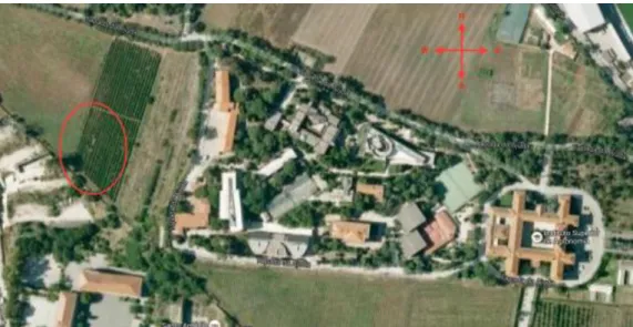
This study was conducted in the educational vineyard of the Instituto Superior de Agronomia, the “Almotivo” vineyard, Tapada da Ajuda, Lisboa, Portugal (figure 1). The experimentation took place during the season of 2016, on the grapevine variety V. vinifera L. cv. Trincadeira.
The vineyard is situated on a small slope, at a latitude of 38˚42’ N and a longitude of 9˚11’ W, at an altitude of approximately 120 meters. The total area of the vineyard is 1 ha, of which around 800 m2 were planted with the cultivar Trincadeira.
The vines were planted in 1998 and grafted on 140Ru (Vitis berlandieri x Vitis rupestris) rootstocks. According to Sarmento (1969), Tapada da Ajuda soils generally present a clay texture and a brown color or, less frequently, reddish-brown especially on soils that are derivative from clay-texture limestone. The soils are majorly originated from basalt or limestone which endured profound alteration from human activity, characterized essentially by great incorporation of organic matter (Matos, 1994). These soils present a depth between 80 and 114 cm, with some rough/coarse elements, including stones and rocks, presenting a clay percentage higher than 30%, with fine limestone (Medina, 1973).
Tapada da Ajuda vineyard is characterized by the influence of the Ocean, therefore there is a Mediterranean climate, which is temperate, with hot and dry summers and cold and humid winters. The average annual precipitation in height is of 674 mm, with maximum monthly rainfall during the winter months (about 113mm) and minimum in the summer months (about 5.5mm).
Figure 1: Aerial Picture of Tapada da Ajuda Vineyard, in Instituto Superior de Agronomia, Lisboa. The red circle indicates the Vinha do Almotivo (source: Google Maps).
18
3.1.1. Site Management
The vines are trained in a vertical shoot positioning system, and pruned with double bilateral Royat cordon, which is supported by the trellis system consisting of wooden posts, with two pairs of movable wires and one fixed wire at the top.
The trunk of the vines had a height of around 70 cm. The vines have an average of 4-5 spurs with 3 buds each and are planted at an inter-row spacing of 2.5 meters and 1.2 meters between the plants in the row. Thus, the density of the plantation can be calculated to 3333 plants/ha and the crop load at around 40,000 buds/ha.
Herbicide was applied on the rows, while a cover crop of natural vegetation was left between the rows. Vines were not irrigated during the growing season.
At pre-flowering, beginning of May, shoot thinning was performed in all the rows so to have 16 to 18 shoots per vine. Afterwards, basal leaves were removed in the early defoliation treatment rows. At the beginning of June, shoot positioning was executed. At the end of the same month, vines were trimmed. Grapes were harvested the first week of September, according with the berry composition parameters (see 3.2.5).
3.1.2. Experimental Design
To determine the impact of basal leaf removal on cluster development and on the berry composition, an early defoliation treatment (ED) was compared with a control non-defoliated (ND). The ED-treatment consisted in the removal of 5 to 6 basal leaves around the cluster zone, at pre-flowering.
The vines were selected according to the vine load: to have a homogeneous pattern, the vines had an average of 7 spurs (minimum 3 and maximum 4 per each arms) with 3 buds each, giving rise to 18 shoots and approximately 6 inflorescences. A load correction was performed on the vines by shoot thinning.
In order to be able to analyze the impact of shoot vigor on the fruit-set, in each of the selected 6 vines, 2 shoots of distinct vigor (2 vigor classes based on their length and diameter: high and low) have been selected for detailed measurements.
At pre-flowering (one week before flowering), the early defoliation treatment (ED) was performed: 6 basal leaves were removed (from the 1st to the 6th shoot node), from all the shoots. No laterals were removed.
19
3.2.
Methodology
3.2.1. Phenological development
From the start of the growing season and along all the vegetative cycle, the phenological stages have been monitored and reported weekly, according to the BBCH-scale (Biologische Bundesanstalt, Bundessortenamt und CHemische Industrie) from Hack et al. (1992), which was adapted to Vitis Vinifera L. by Lorenz et al. (1995).
3.2.2. Leaf Area
Lopes and Pinto method (2005) has been used for the leaf area measurements. This methodology uses the calculated variable Mean Primary Leaf Area (MLA1) to estimate Shoot Primary Leaf Area (PLA). MLA1 is calculated by measuring the biggest leaf (B1) and the smallest leaf (S1) of a shoot to compute the average Leaf area (M1). M1 is multiplied with the counted number of primary leaves of the shoot to calculate MLA1. The same approach was used to estimate Shoot Lateral Leaf Area (LLA) by analogue procedure. The equations used were obtained by Winkler (2016) using cv. Trincadeira, for Shoot Primary Leaf Area:
𝑃𝐿𝐴 = 0.9619238 ∗ 𝑀𝐿𝐴11.01515 Equation 1
and for Shoot Lateral Leaf Area:
𝐿𝐿𝐴 = 1.027245 ∗ 𝑀𝐿𝐴20.97829 Equation 2
LA measurements were performed on the chosen shoots, for a representative sample of 36 shoots per treatment: 2 shoots in every of the 6 selected vines in each row, of which 3 rows for the D-treatment and the other 3 for the ND-D-treatment.
The LA measurements have been carried out periodically: at pre-flowering (the second week of May, one week before the start of flowering, along with the defoliation treatment), at post-flowering (the first week of June; simultaneously a shoot topping was performed and the trimmed parts have been measured as well), at veraison (last week of July), and at complete ripening, concurrently with harvest time.
20
3.2.1. Fruitfulness
In this experimentation, the monitoring of the fruitfulness was done by counting the number of inflorescences per shoot. To assess the number of flowers per inflorescence it was used a non- destructive method based on image analysis. One week before the flowering started, when the inflorescences were swelling, pictures were taken of all the selected clusters, from the selected shoots. Images have been acquired manually under field conditions: each cluster was photographed against a black background, with a digital camera. The distance between the camera and the inflorescences was around 30 to 40 cm.
Meantime, 30 random shoots of Trincadeira grapevine were selected from the adjacent plot; the shoots have been chosen with the condition of having only one cluster each. The images of these 30 clusters have been acquired inside the laboratory. The inflorescences were photographed when entire, and afterwards all the flowers present on the cluster have been individually detached from the rachis and have been photographed as well (methodology adapted from Poni, 2006).
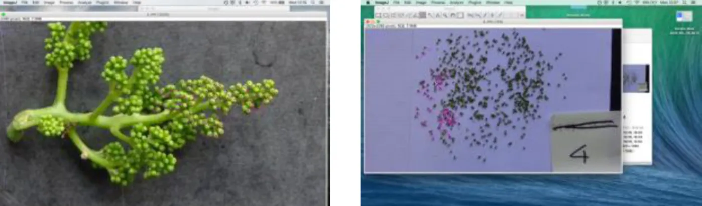
After this operation, using Image Analysis it was possible to estimate the number of flowers of the pictures (figure 2).
Figure 2: Counting of the flowers from the inflorescence with Image Analysis: picture on the left shows the counting on the entire inflorescence; picture on the right shows the counting of the flower of the same inflorescence, after separation.
The main goal was to create a correlation between the number of the flowers which were possible to count on the entire cluster (x variable) and the total number of flowers, after separating them from the rachis (y variable), determining a linear relationship (figure 3).
21
The following equation was obtained using linear regression with least squares method: 𝑦 = 2.4116𝑥 + 0.1252 Equation 3
It was therefore possible to use the Equation 3 to estimate the actual amount of flowers of the selected clusters, from the pictures taken in the field.
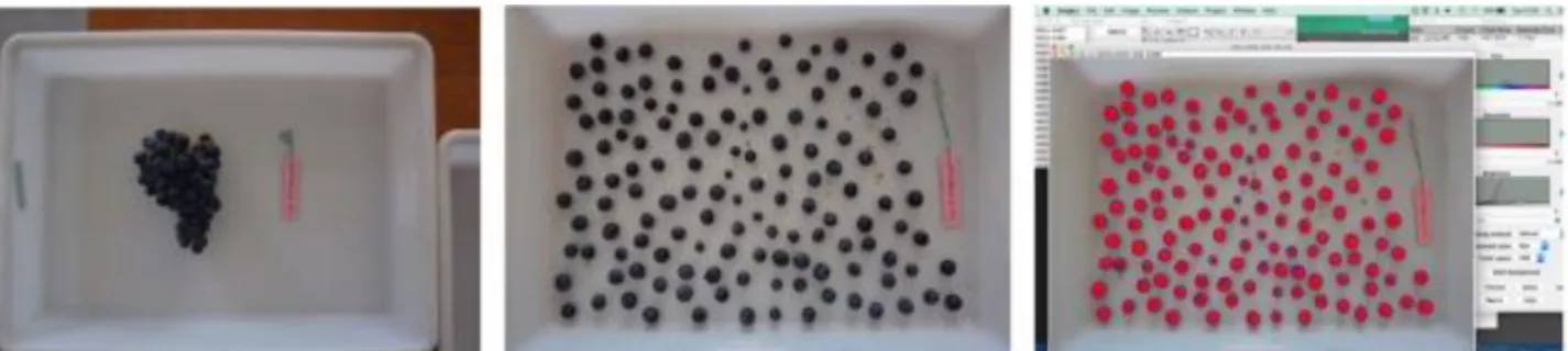
At harvest, all the clusters from selected shoots were collected and analyzed (see section 3.2.8). and the total number of berries per bunch was counted (figure 4). Then the percent fruit-set was estimated using the ratio between number of berries and number of flowers.
Figure 4: Selected cluster photographed at harvest: in the left picture, the entire cluster; in the central picture, the berries of the same cluster, after separation; in the picture on the right, counting the berries with Image Analysis. Figure 3: Linear regression between the number of flowers counted on the entire flower as a predictor (x), and the number of flower counted after separating as a dependent variable or predicted (y).
22
3.2.2. Cluster Light Microclimate
In this experimentation, photosynthetically active radiation (PAR) incident in the vineyard was assessed at the following phenological stages: after flowering, veraison and ripening.
Measurements have been performed with a ceptometer, of the type AccuPAR LP-80, from DECAGON DEVICE.
Ceptometers consist of linear arrays of hemispherical sensors operating simultaneously to register transmitted PAR along a probe of approximately 1 meter. Ceptometers are instruments appropriate for crops planted in rows, since they allow measurements with a limited number of sampling. They are currently use for fIPAR (fraction of intercepted photosynthetically active radiation) and also for LAI estimation (López-Lozano et al., 2013).
Readings have been carried out at several sun elevations during the day: mid-morning (h10.00), midday (around h13.00), and mid-afternoon (h16.00). These timing were as accurate as possible, varying of 30minutes maximum.
Assessments have been performed in each of the six rows: twice at the beginning and twice at the end, with the ceptometer placed parallel to the vineyard facing upwards, in the middle of the inter-row space, so to register the transmitted PAR along the inter-row direction; readings were performed as well inside the canopy in correspondence of every selected vine, in order to register the light incidence in the cluster zone.
3.2.3. Leaf Layer number and Canopy Dimensions
To characterize the vine canopy, the canopy dimensions were measured: the height from the soil to the leaves at the base of the canopy and the height from the soil to the leaves at the top of the canopy were recorded, as well as the width of the canopy in the cluster zone and on the top of the canopy, using a measuring tape.
The leaf layer number was assessed using the Point Quadrat technique (Smart et al., 1988). This method consists in inserting a straight metal stick inside the canopy, horizontally along the cluster zone, and record the contact with the vine features, such as leaves and clusters (shoots were ignored). Recording the contacts as the metal stick advances, and sampling the canopy every 10 cm approximately, it is possible to calculate the percent of gaps, the leaf layer number (LLN), the percent of interior fruit and the percent of interior leaves.
23
3.2.4. Stem Water Potential
In this experimentation, stem water potential (s) measurements have been performed by picking two main leaves per row, in blocks 1 and 2 (rows 13 to 16).
Leaves were previously covered in aluminum foil and a plastic bag, and after two hours (approximately at midday) readings with pressure chamber were executed. This analyses have been repeated during post-flowering, at veraison and at ripening with the aim to characterize to seasonal water status of the vines.
3.2.5. Laboratory Analysis on Grape Composition
Laboratory analyses on grapes have been carried out from the end of July till harvest: at the beginning and at the end of the veraison, at middle ripening, and at full ripening.
Berries were collected from the six selected vines, in each of the selected rows, for a total of six samples of 100 berries each. The weight of every samples has been noted, and afterwards berries were crushed using a gauze, so to separate liquid part (must) from solid parts (skins and seeds). Also, the volume of the must was noted.
The must was then used to measure the pH, the Brix degree, and the titratable acidity (TA).
To the solid parts, ethanol and a buffer solution of tartaric acid (pH=3.2) were added. The quantity in mL of ethanol to be added was calculated with the weight of the berries divided by 8; while the quantity in mL of buffer solution was the result of the volume of must minus the mL of ethanol added. Skins and seeds were therefore left in these solutions for 24 hours; after that anthocyanins and total phenols were calculated.
- pH
The readings were performed with a pH meter (Ribéreau-Gayon et al., 2006). Two determination per sample were carried out.
- TA
Titratable acidity, is determined by neutralization using a solution of sodium hydroxide (NaOH 0.1N), according to the OIV method (Method OIV-MA-AS313-01, Type I method).5 mL of the sampled must are added to 25 mL of boiled water, together with bromothymol blue, the colored agent which changes color at pH 7. The solution is titrated with NaOH 0.1N until the color turns into petrol blue.
24 - °Brix & Potential Alcohol
Brix degree expresses the percentage of sugar in weight and was determined with a refractometer (Carbonneau 1976).
- Anthocyanins
Anthocyanins were estimated with the method proposed by Ribéreau-Gayon and Stonestreet (1965), based on color variation according to bleaching by sulfur dioxide.
A solution containing 1 mL of must, 1 mL of EtOH (0.1% HCl) and 20 mL of HCl at 2% is prepared. From this, two samples are set-up, each with 10 mL of the previous solution; then 4 mL of distilled H2O are added to the first sample and 4 mL of sodium bisulfite (15%) are added to the second. These two solutions are then placed in the spectrophotometer and readings are performed at 520 nm (Ribéreau-Gayon et al., 2006).
- Total Phenols
For the determination of total phenols, the extracted solution was diluted 1/100 in distilled H2O and then readings were performed in the spectrophotometer at 280 nm (Ribéreau-Gayon et al., 2006).
3.2.6. Harvest Protocol
When the grape ripeness was reached, the selected clusters have been harvested (1st September). Each of the selected clusters from the selected shoots was collected in separate plastic bags and identified with the code of the shoot they belonged to, being single cluster per shoot
Entire clusters were weighted, and then the berries were detached from the rachis and separated into healthy and unhealthy (meaning botrytized/dried/dehydrated berries). Weights of rachis, healthy berries and unhealthy berries were measured separately.
Pictures were taken of each entire cluster, of the healthy berries, unhealthy berries, and rachis. Next, the volume of the healthy berries was measured using a measuring cylinder filled with water: berries were immersed and the volume of water displaced was annotated, following Archimedes’ principle.
For what concerns the rachis, its total length was measured, together with the length from the first rachis ramification till the rachis apex, the length from the second ramification till the rachis apex, and the first ramification length. Moreover, all the ramification and the green ovaries were counted, when present.
25 pictures previously taken.
Bunch compactness evaluation has been performed both visually and with the value obtained from the ratio between the berry number and the length of the rachis.
In the field, the measure of diameters of the selected shoots have been assessed.
After the harvest and analyses of the selected clusters, also the other clusters from the selected vines were collected and the weight of the grapes per each plant was evaluated, summing it with the weight of the selected clusters previously collected.
Qualitative analyses for grapes composition have been performed at harvest, as mentioned in section 3.2.5.
3.2.7. Data Analysis
The data collected during the experimentation have been recorded using Excel worksheets (Microsoft Office). The Analytical Software Statistix 9, Analytical Software, USA, was used to perform Analyses of Variance (ANOVA) with the observed data. In the ANOVA, the observed variance of a variable is separated into variation addressed to a factorial variable, such as treatment (ND or ED) or vigor (“High” or “Low”). It provides a statistical test of whether or not the means of several groups of the Randomized Complete Block experimental setup are equal. The F-value is calculated as the quotient of explained variance (Sum of SquaresTREATMENT) to unexplained variance (sum of SquaresERROR).
The computer method calculates the probability (P-value) of a value of F greater than or equal to the observed value. The null hypothesis (H0: “means of the groups are equal”) is rejected if this probability is less than or equal to the chosen significance level (α= 0.05) (Chambers et al., 1992). ANOVA with Factorial analysis (2 factors: defoliation and shoot vigor) was carried out with the data concerning the percentage of fruit set, including interaction effects.
26
4 Results and Discussions
4.1.
Meteorological Data
4.1.1. Weather in 2016
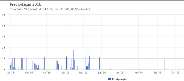
The figures below show the temperature (figure 5) and the precipitation (figure 6) from January until October 2016.
Figure 5: Temperatures (°C) in Lisbon during 2016 year. Red line showing the maximum T°, green line showing the average T°, blue line showing the minimum T°. Data from Instituto Superior Tecnico, Lisbon.