Ocean surface provinces off Southwest Iberia based on satellite remote sensing

LILIAN ANNE KRUG

O

I

SATELLITE REMOTE SENSING

UNIVERSIDADE DO ALGARVE

Faculdade de Ciências e Tecnologia

LILIAN ANNE KRUG

O

I

SATELLITE REMOTE SENSING

Doutoramento em Ciências do Mar, da Terra e do Ambiente (ramo Ciências do Mar, especialidade em Processos e Ecossistemas Marinhos)

Trabalho efetuado sob orientação de: Prof Dra Ana Maria Branco Barbosa Dra Shubha Sathyendranath

UNIVERSIDADE DO ALGARVE

Faculdade de Ciências e Tecnologia

Image: MODIS-Aqua and VIIRS-Suomi NPP composite (March 8, 2017; Credits: Norman Kuring, NASA Earth Observatory)

ii

© Lilian Anne Krug, 2017

A Universidade do Algarve tem o direito, perpétuo e sem limites geográficos, de arquivar e publicitar este trabalho através de exemplares impressos reproduzidos em papel ou de forma digital, ou por qualquer outro meio conhecido ou que venha a ser inventado, de o divulgar através de repositórios científicos e de admitir a sua cópia e distribuição com objetivos educacionais ou de investigação, não comerciais, desde que seja dado crédito ao autor e editor.

iii

T

Science without Borders Programme from the Brazilian National Council for Scientific and Technological Development (237998/2012‐2)

The Foundation of Science and Technology through the project Remote Sensing of Phytoplankton variability off South-Western Iberia: A sentinel for climate change? – PHYTOCLIMA (PTDC/AAC-CLI/114512/2009)

v

“A century from now humanity will live in a managed - or mismanaged - global garden” (Steele et al., 1989). Presently, we worry about what to do about overfishing, ponder possible sub-lethal effect of oil or sewage discharge into the coastal oceans, and are scared by red and brown tides; we discuss the necessity to save some of the tropical forests; we are beginning to control emission of “greenhouse gases” into the atmosphere; and we struggle to calculate how fast and how much the climate will become warmer with and without such controls. A century from now these separate concerns will have been integrated into a single management system because of objective needs, but perhaps also because of broad intolerance of the mismanagement of nature. Obviously, the running of such a controlled system will require massive, continuous data-collecting or monitoring, which will presumably be largely automated. Our great-grandchildren, therefore, will live on a “wired earth” (Steele et al., 1989). Using the data so gathered, however, will demand massive improvements in scientific concepts, and this improvement is already the task for the present generation.

vii

ix

A

I would like to gratefully acknowledge…

… my supervisors Dr Ana Barbosa, Dr Shubha Sathyendranath and Dr Trevor Platt, for giving me constant encouragement and unabridged availability. They are, without a doubt, special people and exceptional mentors. These years were an emotional ride and their guidance was more than crucial. Trevor and Shubha were always supportive, kind and present, even with the physical distance. Ana is the best example I have ever met of a dedicated and ethical researcher, and I cannot think on words to express my gratitude for her.

… the Science without Borders Programme of the Brazilian National Council for Scientific and Technological Development (CsF-CNPq) and the Portuguese Foundation of Science and Technology (FCT), for the financial support. The CsF-CNPq was impeccable during the entire fellowship period and I deeply appreciate the opportunity given to me and to several other Brazilian young researchers.

… the Ocean Colour Climate Change Initiative (European Space Agency), OceanColor (USA’s National Aeronautics and Space Administration), Copernicus Marine Environment Monitoring Service, Ocean Productivity (Oregon University) and every group that works hard to provide free and high quality products for a data-thirsty ocean science community.

… the Marine Microbiology laboratory, the Centre for Marine and Environmental Research and the Faculty of Sciences and Technology of the University of the Algarve, for the space and conditions. In special, I want to thank Paula Caboz from the FCT Secretariat, Dr Oscar Ferreira and Dr Pedro Andrade, former and current directors of the CMTA programme.

… the International Relations and Mobility Office of the University of the Algarve, in particular to Carla Mendes Ferro and Antonio Ramos.

… the International Oceanographic Data and Information Exchange (IODE), the European Space Agency (ESA), the Partnership for Observation of Global Ocean (POGO), the Scientific Committee on Oceanic Research (SCOR), the Surface Ocean - Lower Atmosphere Study (SOLAS) project, the NF-POGO Alumni Network for Oceans (NANO), the Gordon Research Conferences, the Portuguese Estrutura de Missão para a Extensão da Plataforma Continental (EMEPC) and other international organizations that provided me with resources to attend trainings and scientific events, allowing me to acquire and improve the techniques used in this thesis, as well as to present and discuss its partial results with my peers and renowned experienced researchers.

… the good-hearted people whose assistance was essential at some point along this thesis, including Mimoy, Paul, Dr Forough Fendereski, Dr Tom Jackson, Dr Tim Moore, Cátia L., Cátia G., Dr Rita Domingues, Dr Helena Galvão, Dr Joaquim Luis, Dr Paulo Relvas.

x

…. my Portuguese family (Cátia, Liliana, Sara, João, Paul, Giammi, Gui, Maria Rita, Camilla and Lucas), the ‘BBF’ Mari and my beloved goddaughter Nina, my suffering buddy ‘Frá’ (YES, we did it!), the ‘xu’ to my ‘xu’ Diego, MyLadies (Ellenzinha, Eurídice and Sara) and the rest of the gym gang, the NANO/POGO team (Sophie, Vikki, Laura and Olga), Dr Murray Brown, Dr Greg Reed, Rituxa, Ana Matias, Chiqui, Cat, Filipe, Carlos, Maria, Sandrinha, Sónia, Thi, Malão, Tati, Alex, Nathália, my lab hermano and coffee dealer Fran, Dna Maria do Carmo and Seu José, for the 24/7 emotional support system and guaranteed laughs.

…. my entire family, but in particular to my parents Osmar and Roseli, siblings Lian, Dan and Alethéa, sisters-in-law Denise and Ivy, nieces Ashley and Giuliana, nephew Enzo, aunt Wilma and my grandparents Alberto, Judith (in memoriam), Lino (in memoriam) and Margarida (in memoriam). Thank you for the unconditional love and for believing in me, supporting every single step in my professional and personal journeys even though it meant I gradually move farther and farther away from home and couldn’t visit for 3 long years or couldn’t properly say goodbye. À toda a minha família, mas especialmente aos meus pais

Osmar e Roseli, aos meus irmãos Lian, Dan e Alethéa, às minhas cunhadas Denise e Ivy, minhas sobrinhas Ashley e Giuliana, meu sobrinho Enzo, tia Wilma, meus avós Alberto, Judith (in memoriam), Lino (in memoriam) e Margarida (in memoriam). Muito obrigada pelo amor incondicional e por acreditarem em mim, apoiando cada passo da minha jornada profissional e pessoal, mesmo que isto significasse eu me mudar cada vez mais longe de casa, por três longos anos sem poder visitá-los, ou sem poder me despedir apropriadamente. Amo vocês.

xi

A

This thesis aimed to partition the complex surface marine domain off Southwest Iberia Peninsula (SWIP), using satellite remote sensing, and use it to assess phytoplankton variability patterns and underlying environmental drivers (1997 – 2015). Three unsupervised partition strategies, based on distinct input databases and temporal representations, detected a variable number of partition units (regions, provinces) of singular environmental and phytoplankton patterns within SWIP. An abiotic-based partition delineated 12 dynamic Environmental Provinces (EPs) that alternated coverage dominance along the annual cycle. EP patterns were in general related to phytoplankton biomass, indicated by satellite chlorophyll-a concentration (Chl-a), and productivity, thus supporting the biological relevance of this abiotic-based partition. A static partition, based on the main variability modes of Chl-a, derived 9 Chl-a regions. Moreover, a static partition strategy synthesised phytoplankton phenological patterns over SWIP into 5 phenoregions, with coherent patterns of timing, magnitude and duration of blooms. The spatial distribution of EPs, Chl-a regions and phenoregions shared similarities, which can be considered the main spatial patterns of SWIP ocean surface. In general, the spatial arrangement of the partition units showed a separation between coastal and open ocean, a latitudinal division (ca. 36.5oN) over the open ocean and, over the coast and slope, the influence of coastal upwelling along the west Portuguese coast and Cape São Vicente, and of river discharge along the northeastern Gulf of Cadiz. The environmental drivers of phytoplankton varied across partition units. Water column stratification, riverine discharge and upwelling intensity were the most influential modulators, and large scale climate indices usually showed minor effects. Environmental variables, Chl-a and phenology showed significant seasonal variability patterns, varying across regions. Interannual patterns were more complex, and significant trends were mostly detected within the Gulf of Cadiz. Linkages between environmental variability and phytoplankton support their use as an indicator of ecosystem status and change.

Keywords: ocean surface partition, satellite remote sensing, unsupervised classification, environmental variability, phytoplankton variability, phytoplankton phenology

xiii

R

O oceano superficial é um domínio extremamente complexo e dinâmico, onde as interações com a atmosfera e o continente modulam a distribuição e atividade dos organismos marinhos e o clima da Terra. O fitoplâncton, principal produtor primário marinho, é fortemente influenciado pelos processos atuantes no oceano superficial, constituindo um importante indicador do estado e variabilidade dos ecossistemas marinhos. Assim, a organização espacial horizontal do oceano superficial, função da variabilidade das propriedades abióticas e comunidades biológicas (incluindo o fitoplâncton), apresenta uma série de unidades funcionais distintas (regiões ou províncias), com atributos e padrões de variabilidade específicos. A partição ou regionalização do oceano, com identificação e delimitação destas unidades funcionais, simplifica a complexidade do oceano superficial e representa uma ferramenta para avaliar e compreender o funcionamento do oceano superficial, apresentando diversas aplicações ao nível do estudo, gestão e conservação dos ecossistemas marinhos. A deteção remota por satélite constitui uma fonte valiosa de dados para a partição do oceano superficial, pois disponibiliza campos sinóticos de várias variáveis oceanográficas e atmosféricas, em escalas espacial e temporal pertinentes, abrangendo períodos de várias décadas.

A presente tese pretende particionar o complexo domínio marinho superficial do sudoeste da Península Ibérica (Southwest Iberia Peninsula, SWIP), com base em deteção remota por satélite, e avaliar a variabilidade do fitoplâncton e forçadores ambientais associados em regiões específicas (unidades funcionais) da área de estudo. Para atingir os objectivos principais foi inicialmente efetuada uma revisão do conhecimento científico sobre as estratégias de partição do oceano superficial baseadas em deteção remota por satélite (Capítulo 2) e, posteriormente, foram aplicadas diversas estratégias de partição não-supervisionadas à área de estudo (Capítulos 3 - 5). Tais estratégias permitiram particionar a área de estudo com base em diferentes caraterísticas do oceano superficial (propriedades abióticas, variação da concentração de clorofila-a e índices fenológicos do fitoplâncton) e diferentes abordagens metodológicas (métodos de partição e resolução temporal). As diferentes partições do SWIP foram utilizadas para avaliar os padrões de variabilidade da biomassa e fenologia do fitoplâncton e suas relações com diferentes forçantes ambientais. No contexto deste estudo, as variáveis ambientais avaliadas incluíram variáveis locais indicadoras do ambiente físico, químico e ótico, variáveis hidrológicas indicadoras de processos costeiros

xiv

(descarga dos rios e intensidade do afloramento costeiro) e indicadores climáticos de larga escala.

A revisão do estado do conhecimento na área da partição do oceano superficial em unidades funcionais (Capítulo 2) mostrou que a evolução das estratégias de partição acompanhou o desenvolvimento dos produtos de deteção remota da cor do oceano, os quais permitiram a definição de partições dirigidas à avaliação dos ecossistemas marinhos. Com base nesta revisão, as estratégias de partição do oceano superficial devem idealmente considerar os seguintes elementos: (i) objetivos e aplicações; (ii) critérios e dados de entrada; (iii) métodos de partição; e (iv) escalas espaciais e temporais. Para cada um dos elementos referidos, as abordagens utilizadas na literatura científica foram estruturadas e sumarizadas. A utilização do SWIP como um estudo de caso, com análise das partições prévias que contemplaram esta área, demonstrou que as estratégias que aplicaram uma resolução espacial de mesoescala e métodos de delineamento não supervisionados foram mais adequadas para discriminar os principais processos forçadores do fitoplâncton na área de estudo. Assim sendo, estas abordagens foram consideradas nas três estratégias de partição aplicadas na tese.

A partição dinâmica do SWIP, baseada na técnica não-supervisionada de Agrupamento Aglomerativo Hierárquico (Hierarchical Agglomerative Clustering, HAC), utilizou variáveis abióticas adquiridas a partir de deteção remota por satélite e modelos computacionais para o período de 2002 a 2011 (Capítulo 3). Inicialmente foram utilizadas 22 variáveis abióticas, representativas dos ambientes físico, químico e ótico do SWIP, com uma resolução temporal e espacial de 16-dias e 4 km, respetivamente. Esta estratégia de partição delineou doze Províncias Ambientais dinâmicas (Environmental Provinces, EP), sendo 2 predominantemente costeiras, 2 predominantemente localizadas sobre o talude continental e 8 predominantemente oceânicas. A distribuição espacio-temporal e as propriedades abióticas das EP, bem como sua relevância biológica, foram avaliadas. Durante o ciclo anual, foi detetada uma alternância na extensão e área de cobertura das EP, as quais foram agrupadas de acordo com o período de predominância: frio (outono-inverno) ou quente (primavera-verão). As EP predominantes durante o período frio apresentaram maior variabilidade, especialmente na área central oceânica do SWIP, enquanto as EP predominantes durante o período quente foram mais estáveis em termos de cobertura de área. As propriedades abióticas das EP refletiram os processos oceanográficos e costeiros predominantes dos domínios. Por exemplo, as EP de período quente dominante sobre o talude continental e costa oeste apresentaram

xv

ventos meridionais fortes e intensificação do transporte de Ekman perpendicular à costa, ambos indicativos de aumento de intensidade de afloramento, típico neste período do ano. Adicionalmente, a avaliação da relevância biológica desta partição abiótica indicou diferenças significativas nas propriedades fitoplanctônicas das EP bem como similaridades entre os padrões espaciais desta partição e da partição baseada na abundância do fitoplâncton (resultante da estratégia aplicada no Capítulo 4). Tal resultado demonstrou que a classificação baseada exclusivamente em propriedades abióticas pode representar uma ferramenta valiosa para avaliar propriedades ambientais e estruturas ecológicas.

A segunda estratégia consistiu em uma partição estática do SWIP, baseada nos principais modos de variabilidade espacio-temporal da concentração de clorofila-a (Chl-a), indicadora da biomassa total de fitoplâncton (Capítulo 4). Esta partição utilizou a Chl-a derivada a partir de deteção remota por satélites, durante um período de 15 anos (1997-2012). Os modos dominantes de variabilidade da Chl-a foram extraídos através da análise das Funções Ortogonais Empíricas (Empirical Orthogonal Functions, EOF). Esta estratégia de partição identificou e delineou 9 regiões (Chl-a regions), 4 costeiras, 2 sobre ao talude continental e 3 oceânicas. A aplicação de modelos aditivos generalizados a cada Chl-a region permitiu identificar os forçadores ambientais relevantes para a previsão da Chl-a em cada região, bem como os seus padrões de variabilidade intra-anuais e interanuais. O poder de previsão dos modelos regionais bem como as forçantes ambientais que os integram variaram marcadamente, apresentando melhor performance para o oceano aberto. As variáveis ambientais locais (ex.: temperatura da superfície do oceano, radiação fotossinteticamente ativa) emergiram como os preditores mais influentes em todas as Chl-a regions, enquanto os indicadores de padrões climáticos de larga escala apresentaram efeitos secundários mas ainda significativos. De modo geral, os modelos preditivos das Chl-a regions oceânicas indicaram a estratificação da camada superficial como principal fator relacionado ao aumento da disponibilidade de nutrientes. Para as regiões costeiras e sob o talude continental, as descargas fluviais e o afloramento costeiro representaram fontes adicionais de nutrientes. Padrões internanuais significativos, e opostos, foram detetados apenas nas regiões localizadas a sul de 37ºN, com um aumento de Chl-a na região oceânica e um declínio na zona costeira e talude continental. Estes padrões foram acompanhados por um aumento significativo na velocidade do vento e na profundidade da camada de mistura, nas mesmas Chl-a regions, os quais podem ter aumentado a disponibilidade de nutrientes e reduzido a intensidade média da luz na camada de mistura.

xvi

A terceira e última estratégia de partição aplicada (Capítulo 5) baseou-se nas propriedades fenológicas do fitoplâncton no SWIP, durante um período de 18 anos (1997-2015), e foi desenvolvida com base na aplicação da técnica não-supervisionada HAC. Os índices fenológicos foram derivados a partir de dados de Chl-a, obtidos por deteção remota por satélite, e incluíram o número de blooms por ano, a duração total de blooms por ano, duração média dos eventos, valor máximo de Chl-a, e datas do início, pico e término dos blooms. Esta estratégia de partição estática delineou 5 fenoregiões (phenoregions), 3 localizadas sobre a costa e talude continental e 2 oceânicas. No oceano, o fitoplâncton apresentou um único

bloom por ano, com reduzida intensidade e longa duração, geralmente iniciado em Novembro.

Este bloom iniciou maioritariamente durante o período de aumento da profundidade da camada de mistura, possivelmente devido ao aumento da disponibilidade de nutrientes. Pelo contrário, as fenoregiões costeiras apresentaram uma elevada variabilidade intra-anual, consequência da ocorrência de múltiplos blooms ao longo do ano, intensos e com duração e data de ocorrência variáveis. Nas regiões costeiras, as relações entre a fenologia do fitoplâncton e os forçadores ambientais foram mais complexas, especialmente na fenoregião

Upwelling-influenced. Nesta, os blooms ocorreram maioritariamente em dois períodos, no

final do inverno, início da primavera e durante a estação favorável ao afloramento costeiro (Maio-Setembro), reduzindo as associações significativas entre a intensidade do afloramento e os índices fenológicos. Nas restantes fenoregiões costeiras (Coastal-slope e

River-influenced), a descarga do rio Guadalquivir representou um regulador significativo da

frequência de blooms por ano, bem como da sua intensidade, duração e datas de início. Todas as fenoregiões, exceto uma (Oceanic), apresentaram padrões interanuais significativos, para pelo menos um dos índices fenológicos. Nas fenoregiões localizadas na área costeira e de talude continental, foi detetado um aumento linear na duração dos blooms de fitoplâncton e sua fase de desaceleração, enquanto a fenoregião River-influenced apresentou padrões significativos para as datas dos blooms. Adicionalmente, os índices climáticos de larga escala (AMO, NAO e WeMO) correlacionaram-se com os padrões fenológicos em todas as fenoregiões exceto na Upwelling-influenced.

De modo geral, a distribuição espacial das unidades de partição identificadas com base nas três estratégias de partição utilizadas na presente tese (EP, Chl-a regions e fenoregiões) apresentou similaridades, as quais podem ser consideradas os principais padrões espaciais do oceano superficial no SWIP. Apesar da identificação de um número variável de unidades de partição em função da estratégia aplicada, a organização espacial das mesmas destacou uma

xvii

separação gradual entre a costa, talude continental e oceano aberto, e uma divisão latitudinal (cerca de 36.5ºN) no último. Nas áreas sobre a costa e talude continental, as partições destacaram ainda as influências do afloramento costeiro, ao longo do setor oeste de Portugal e Cabo São Vicente, e da descarga fluvial, ao longo do setor nordeste do Golfo de Cadiz. A estratificação da coluna de água, a descarga dos rios Guadiana e Guadalquivir e a intensidade do afloramento costeiro na costa oeste de Portugal foram os fatores ambientais mais influentes nos padrões de variabilidade do ambiente abiótico e na biomassa e fenologia do fitoplâncton no SWIP. Todas as estratégias de partição detetaram uma variabilidade intra-anual significativa, a nível das variáveis abióticas e do fitoplâncton. Nas regiões oceânicas, a Chl-a apresentou um valor máximo anual no final do inverno/início da primavera, gerado pelo aumento da profundidade da camada de mistura e consequente aumento da concentração de nutrientes inorgânicos dissolvidos. Nas regiões costeiras, a variabilidade intra-anual da Chl-a foi mais complexa e apresentou um máximo secundário durante o verão em áreas sob a influência do afloramento costeiro. Em geral, a forte sazonalidade refletiu os efeitos da variabilidade de larga escala no forçamento atmosférico. Estas alteram a circulação do oceano superficial e os processos costeiros, afetando a disponibilidade de nutrientes e luz e, consequentemente, o crescimento líquido do fitoplâncton.

Em relação à variabilidade intra-anual, a variabilidade interanual da cobertura das EP e do fitoplâncton apresentou padrões mais complexos e as regiões com padrões significativos localizaram-se, principalmente, na área do Golfo de Cadiz. Nesta zona, entre o período entre 2002 e 2006, a percentagem da área de cobertura das EP localizadas sobre as áreas costeiras e de talude continental tendeu a diminuir, em simultâneo com o aumento da área das EP oceânicas, fato que pode associar-se à redução do caudal fluvial. A variabilidade interanual da Chl-a também apresentou tendências opostas nas zonas costeira e oceânica do Golfo de Cadiz, com um declínio nas Chl-a regions costeiras e de talude continental e um aumento na Chl-a

region oceânica. Na fenoregião influenciada pela descarga dos rios, foi ainda detetado um

atraso nas datas do início, pico e término dos bloom. A variabilidade ambiental não mostrou relações claras com os padrões fenológicos, embora a diminuição observada na descarga dos rios possa explicar o atraso nas datas dos blooms, devido à redução na disponibilidade de nutrientes. Dos índices de padrões climáticos de larga escala, AMO, NAO e WeMO destacaram-se como forçantes significativos de variações no fitoplâncton para o SWIP, com influências variáveis de acordo com a unidade de partição. De modo geral, AMO atuou mais significativamente sobre os domínios oceânico e do talude continental, a NAO apresentou

xviii

relações com o fitoplâncton sobre as regiões a sul de 36.5oN e o WeMO relacionou-se significativamente com os padrões de fitoplâncton nas unidades de partição localizadas na zona de influência dos rios.

Considerando as relações entre o fitoplâncton e os forçadores ambientais identificadas na presente tese, é expectável que as alterações do clima previstas para o SWIP e região nordeste do Oceano Atlântico (ex.: redução da precipitação, aumento da frequência de ondas de calor, da temperatura da superfície do mar) afetem a variabilidade ambiental e o fitoplâncton de forma variável nas várias regiões identificadas no SWIP. A deteção de variações interanuais, bem como a diferenciação entre variações “naturais” e associadas à variabilidade climática, dependerá, contudo, da complexidade da região. De acordo com os resultados desta tese, estas alterações deverão ser mais facilmente detectadas nas regiões oceânicas do SWIP, domínio que apresentou relações menos complexas do SWIP. No entanto, a discriminação entre o efeito da variabilidade climática versus variabilidade natural requererá a análise de séries temporais mais extensas que as exploradas neste estudo. Globalmente, as estratégias de partição utilizadas na presente tese representam metodologias objetivas, reprodutíveis e de custo reduzido, que podem ser aplicadas em diversos ecossistemas marinhos. Adicionalmente, as partições do do oceano superficial podem ser aplicadas com objetivos distintos, incluindo o estudo de processos oceanográficos específicos ou a gestão e conservação de recursos e ecossistemas marinhos. No geral, este estudo evidenciou uma relação significativa entre o fitoplâncton e a variabilidade ambiental no SWIP, suportando a utilização do fitoplâncton como indicador do estado do ecossistema e como elemento-chave para avaliar as respostas dos ecossistemas à variabilidade e alterações climáticas.

Palavras-chave: partição do oceano superficial, deteção remota por satélites, classificação não-supervisionada, variabilidade ambiental, variabilidade do fitoplâncton, fenologia do fitoplâncton.

xix

T

Acknowledgements ... ix Abstract ... xi Resumo alargado ... xiii Table of contents ... xix List of figures ... xxiii List of tables ... xxxiii

CHAPTER 1.GENERAL INTRODUCTION ………...……….. 1

1.1 Ocean surface partition ………. 3

1.2 Satellite remote sensing ………..……….. 5

1.3 Thesis objectives ………..……… 8

1.4 Thesis outline ………...… 8

CHAPTER 2. OCEAN SURFACE PARTITIONING STRATEGIES USING OCEAN COLOUR

REMOTE SENSING: A REVIEW ……….……...…..…………. 9

Abstract ………..…………...……. 11

2.1 Introduction ………..………...…. 12

2.2 Historical background of ocean surface partitioning using Ocean Colour

Remote Sensing ………. 14

2.3 Aims and uses of partitioning ……….………..… 15

2.4 Partition variables and/or criteria (input dataset) ……….…….………... 19

2.5 Delineation methods ………...……….. 23

2.6 Spatial coverage and temporal representation ………..……… 26 2.7 Study case: partitioning areas off South West Iberian Peninsula ………. 29 2.8 Concluding remarks and future directions ………... 34

CHAPTER 3. DELINEATION OF OCEAN SURFACE PROVINCES OVER A COMPLEX

MARINE DOMAIN (OFF SWIBERIA): AN OBJECTIVE ABIOTIC-BASED APPROACH …… 37

Abstract ………... 39

3.1 Introduction ……….. 40

3.2 Materials and Methods ………. 42

3.2.1 Study area ………..………. 42

3.2.2 Input datasets ……….. 43

3.2.2.1 Physical environment ……… 44

3.2.2.2 Optical environment ……….. 45

3.2.2.3 Chemical environment ……….. 45

3.2.2.4 Indicators of local and remote forcing .………. 46

3.2.3 Data analyses ……….. 47

3.2.3.1 Data pre-processing ………... 48

3.2.3.2 Data reduction ………... 49

3.2.3.3 Delineation of provinces ………... 49

3.2.3.4 Analysis of province-specific spatial-temporal variability patterns and

xx

3.2.3.5 Assessment of the biological significance of the partition ………...….... 51

3.3 Results ………...…….. 52

3.3.1 Delineation of environmental provinces off SW Iberia …………...……….. 52 3.3.1.1 Selection of input variables ………..………. 52 3.3.1.2 Data reduction and cluster analysis ……….………. 53 3.3.2 Environmental provinces off South Western Iberia ……….……... 54 3.3.2.1 Spatial-temporal distribution patterns of environmental provinces ….…. 54 3.3.2.2 Province-specific environmental properties ………..… 60 3.3.3.3 Assessment of the biological relevance of the partition ………... 63

3.4 Discussion ………...….... 65

3.4.1 Environmental provinces off SW Iberia and previous partitions of the study

area ………...…….. 66

3.4.2 Spatial-temporal dynamics of environmental provinces ………..…..… 68 3.4.3 Abiotic properties of environmental provinces ………..…….... 71 3.4.4 Biotic relevance of the abiotic-based environmental provinces ………..…... 72

3.5 Conclusions ………...……. 74

CHAPTER 4. UNRAVELLING REGION-SPECIFIC ENVIRONMENTAL DRIVERS OF

PHYTOPLANKTON ACROSS A COMPLEX MARINE DOMAIN (OFF SWIBERIA)………… 77

Abstract ………...….. 79

4.1 Introduction ………...….. 80

4.2 Materials and Methods ………. 83

4.2.1 Study area ……….……. 83

4.2.2 Phytoplankton data ………..….……. 85

4.2.3 Environmental data ………. 86

4.2.3.1 Ocean physical and chemical variables ………..…..…… 86

4.2.3.2 Upwelling intensity ………..….…... 88

4.2.3.3 Hydrographic and meteorological variables ………..……..…. 89

4.2.4 Data analyses ………..…..…….. 90

4.2.4.1 Empirical Orthogonal Function analysis and study area regionalization . 91 4.2.4.2 Region-specific phytoplankton temporal variability patterns and

environmental drivers ………..……….… 92

4.3 Results ……….. 94

4.3.1 Large-scale environmental setting off SW Iberia ……….…...…... 94 4.3.2 Large-scale phytoplankton variability patterns off SW Iberia ……….…..… 97 4.3.3 Dominant modes of chlorophyll-a variability off SW Iberia ……….… 98 4.3.4 Region-specific phytoplankton temporal variability patterns ……… 100 4.3.5 Region-specific phytoplankton environmental drivers ………....…….. 104

4.4 Discussion ………...….… 111

4.4.1 Phytoplankton seasonal variability patterns and underlying environmental

drivers ……….……… 112

4.4.2 Phytoplankton interannual variability patterns and linkages to climate

variability ……….…..……. 116

4.5 Conclusions ………....…….. 121

CHAPTER 5. PHYTOPLANKTON PHENOLOGY PATTERNS OFF SW IBERIA (NE ATLANTIC): A STRATEGY FOR OBJECTIVE PARTITIONING OF A COMPLEX MARINE

DOMAIN………....…… 123

xxi

Abstract ………...……….…….. 125

5.1 Introduction ………...……….…….. 126

5.2 Materials and methods ………...……….……. 129

5.2.1 Study area …………..………..……….……. 129

5.2.2 Phytoplankton chlorophyll-a concentration ………..……. 131

5.2.3 Optical variables ………..………….. 132

5.2.4 Physical and chemical variables …...………..……….….. 132 5.2.5 Upwelling intensity and hydrographic variables …...………..…...… 133 5.2.6 Large scale climate indices ...……….…. 134

5.2.7 Data analyses ……….. 135

5.2.7.1 Phytoplankton phenological indices ….………..…..… 136 5.2.7.2 Delineation of phenology-based regions off SW Iberia .………... 137 5.2.7.3 Region-specific phenological properties, interannual variability patterns

and environmental determinants ………..………....………. 138

5.3 Results ………....…….. 140

5.3.1 Phytoplankton phenology off SW Iberia: a pixel-based assessment ……... 140 5.3.2 Phenology-based partition off SW Iberia ………..……. 142 5.3.3 Phytoplankton phenology off SW Iberia: a phenoregion-based assessment .. 144 5.3.4 Region-specific drivers of bloom phenology off SW Iberia ………….…... 149

5.4 Discussion ………...…….... 154

5.4.1 Phenology-based partition of the marine domain off SW Iberia …….…….. 155 5.4.2 Phytoplankton phenological patterns off SW Iberia ………..……… 156 5.4.3.Phytoplankton phenology off SW Iberia: interannual patterns and

environmental drivers ……….. 160

5.4.3.1 Open ocean phenoregions ………... 161

5.4.3.2 Coastal phenoregions ……….………... 163

5.5 Conclusions ……….. 167

CHAPTER 6.CONCLUDING REMARKS ..………..…… 169

6.1 General conclusions ……….…… 171

6.2 Recommendations and future perspectives ………..… 174 CHAPTER 7.REFERENCES ………..…………... 177 APPENDIX A……….…………..…. 235 APPENDIX B……….………...… 241 APPENDIX C……….………...… 249 APPENDIX D……….………...… 263

xxiii

L

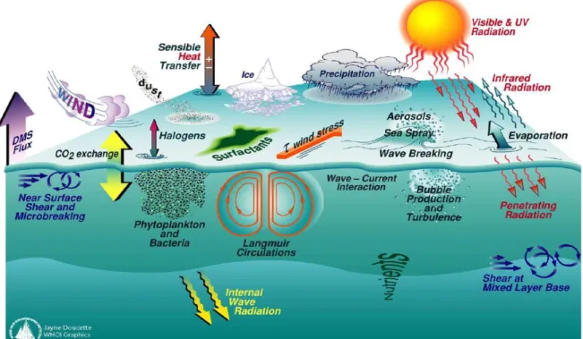
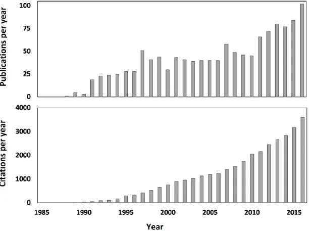
Figure 1.1 Schematic representation of multiple processes occurring in the ocean surface, results of its interactions with adjacent deeper layer and atmosphere. Adapted from original image by Jayne Doucette (Woods Hole Oceanographic Institute) ...……….. 3 Figure 1.2 Evolution of (top) the number of indexed articles using and the terms “ocean surface” and “provinces or regions or partitions” and (bottom) the number of citations of these articles, between 1980 and 2016, extracted from the Web of Science database, as in 16 August 2017 ……… 5

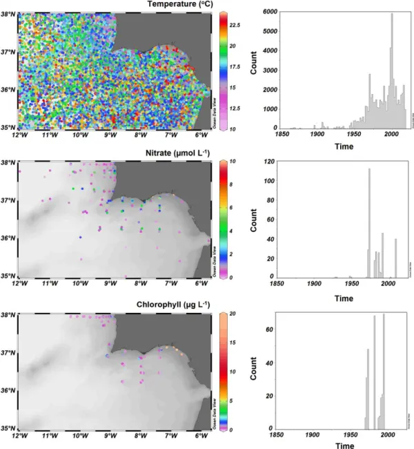
Figure 1.3 Spatial (right) and temporal (left) distribution of in situ ocean surface (0 - 5 m depth) temperature, nitrate and chlorophyll-a data off the Southwest Iberian Peninsula (SWIP), sampled between 1864 and 2013 and available at the World Ocean Database (Boyer et al., 2013) ……….………. 6

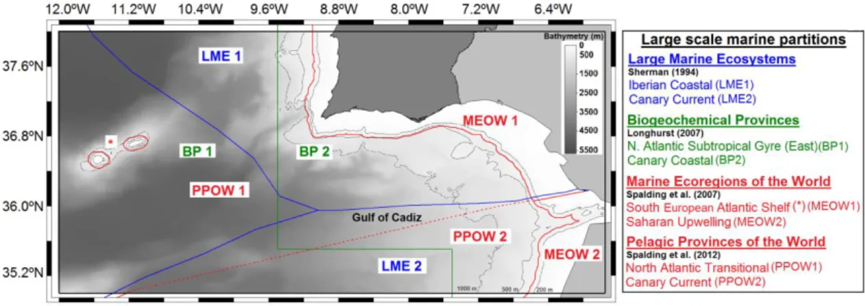
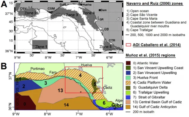
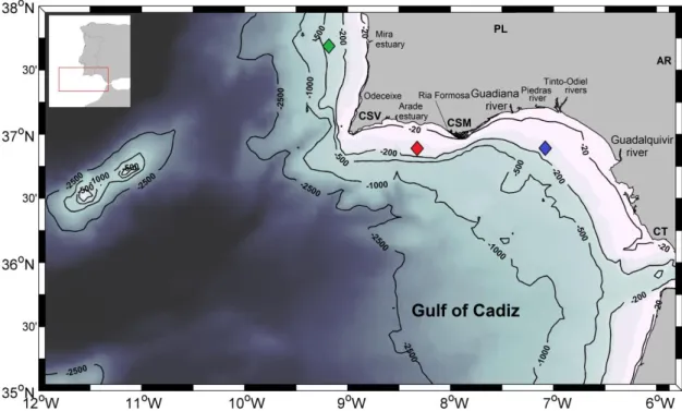
Figure 2.1 Global ocean surface partitions for the domains off South West Iberian Peninsula (NE Atlantic) with overlaid bathymetry (General Bathymetric Chart of the Oceans, GEBCO_2014 Grid, version 20150318, http://www.gebco.net). Large Marine Ecosystems and Biogeochemical Provinces shapefiles downloaded from Claus et al. (2016). Marine Ecoregions and Pelagic Provinces of the World shapefiles provided by The Nature Conservancy (2012) ………..………. 31 Figure 2.2 Representation of spatial functional units in the Gulf of Cadiz (NE Atlantic) associated to mesoscale-level partition studies, based on spatial empirical orthogonal function analysis. (A) Zones of distinct phytoplankton variability patterns (left) and respective designations (right). Source: adapted from Navarro and Ruiz (2006). (B) Gulf of Cadiz section of the regionalization of marine waters of the South Iberia Peninsula (left) and designations (right). Source: adapted from Muñoz et al. (2015). The red rectangle represents the approximate area of interest (AOI) of Caballero et al. (2014). See the text for further details ……….………. 33 Figure 3.1 The southwest area off the Iberian Peninsula (SWIP) bathymetry and main

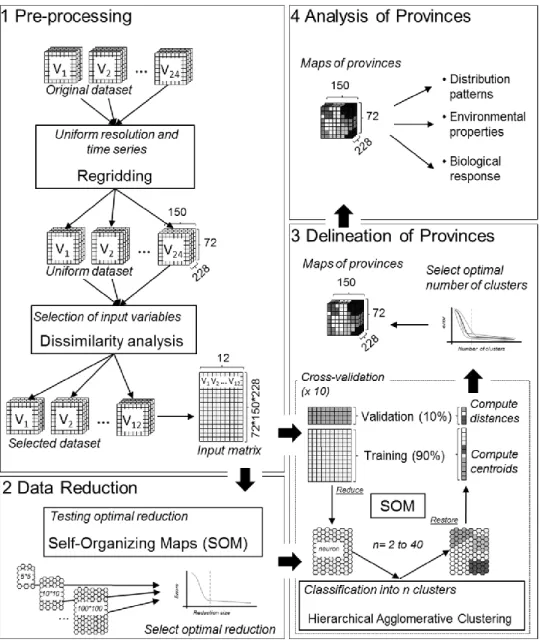
sources of freshwater discharges. CSV, CSM and CT depict the location of prominent topographic features, Cape São Vicente, Cape Santa Maria and Cape Trafalgar, respectively. PL and AR depict the location of Pulo do Lobo and Alcalá del Río hydrographic stations, respectively. Diamonds show the position of pixels used for the calculation of Cross Shore Ekman Transport for the West Coast (green), and west (red) and east Cape Santa Maria sectors (blue). Location of the outflow of major estuarine systems is also shown (see text for further details) ……….…. 43 Figure 3.2 Flow diagram representing the four steps associated to the delineation of environmental provinces in the area off South West Iberian Peninsula: 1 - Data pre-processing; 2 - Data reduction; 3 - Delineation of Provinces; and 4 -

xxiv

Analysis of Provinces. See text for further details ……….…. 48

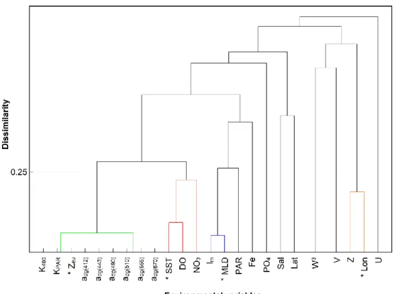
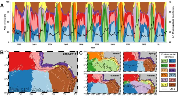
Figure 3.3 Dissimilarity analysis based on variables representative of the abiotic environment off SW Iberia, during the 2002-2011 period. Coloured nodes indicate groups with dissimilarity values below the defined threshold (0.25), and * denotes the variables selected to represent each group. Variables include: K490 = Light attenuation at 490 nm coefficient, KPAR = photosynthetically available radiation attenuation coefficient, Zeu= euphotic depth, adg(λ) = absorption by detrital and coloured dissolved organic matter coefficient at specific wavelengths, SST = sea surface temperature, DO = subsurface dissolved oxygen, NO3 = subsurface nitrate concentration, MLD = mixed layer depth, Fe = subsurface iron concentration, PAR = photosynthetically available radiation, PO4 = subsurface phosphate concentration, Sal = subsurface salinity, Lat = latitude, V = meridional component of wind, W3 = turbulent mixing index, Z = bathymetry, Lon = longitude and U = zonal component of wind ………..…. 53 Figure 3.4 Spatial and temporal dynamics of the 12 environmental provinces (EPs, see colours) delineated off the South West Iberian Peninsula, during the period February 2002 - December 2011. (A) Temporal variability of the relative area coverage of the EPs (as % of the study area). (B) Province modal maps for the whole time series, and (C) Season-specific province modal maps. Black lines represent average surface chlorophyll-a concentration (Chl-a, µg L-1) for the study area (A, B) or period (C). White lines (B, C) are isobathymetric contours (200m, 500m, 1000m and 2500m) ………..…. 55 Figure 3.5 Seasonal distribution of the occurrence (pixel-based frequency, as %) of the 12 environmental provinces (EPs) delineated off the South West Iberian Peninsula, during the period February 2002 - December 2011, organized into four groups (I, II, III, and IV), based on their prevailing season(s) of occurrence. Season-specific EP core maps, based on occurrence frequencies equal to, or higher than, 40%, are depicted at the bottom (white areas: EPs frequency < 40%) ………..…………. 57 Figure 3.6 Partial effects of intra-annual (expressed as month) and interannual variability (expressed as year) on the area coverage of the 12 environmental provinces (EP) off Southwest Iberia Peninsula (period: 2002-2011), derived from generalized additive mixed models (GAMMs). EPs are organized into four groups (I, II, III, and IV), based on their prevailing season(s) of occurrence. Model explanatory power (as % explained variance) is shown next to each EP designation (in parenthesis), and the significance level (p-value) of each predictor (month, time) is denoted by asterisk symbols (top right), where *, **, *** indicate p-value <0.05, <0.01 and <0.001, respectively. For each plot, predictor values are represented on the x-axis, where short vertical lines indicate the exact predictor observations. Values on the y-axis represent the partial effects of the specific predictor, holding the other predictor constant. Numbers in parentheses on the y-axis represent the effective degrees of freedom (edf), indicative of the smoothness of each function; values of edf equal to 1 represent a linear effect of the predictor, and values higher than 1 indicate progressively stronger non-linear effects. Solid lines indicate the

xxv

smoothed non-parametric trends, and gray shaded areas designate the point-wise 95% confidence intervals. Regions where the 95% CI bands enclose the x-axis line indicate no significant effects of the prediction. At each stage, the value of the EP areal coverage is given by the sum of the partial effects of both predictors plus a constant (see Table B.1 for detailed statistics) ………..…... 59

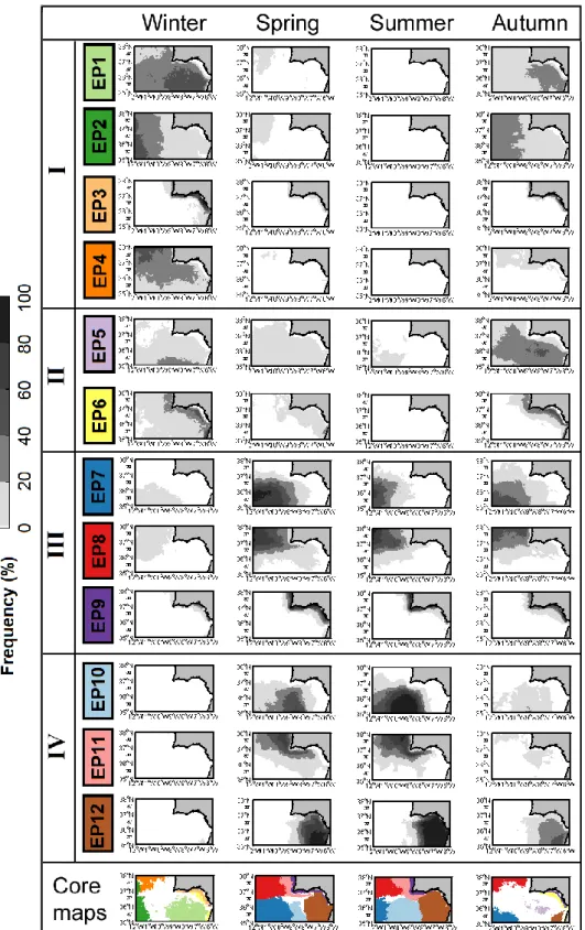
Figure 3.7 Characterization of each of the 12 environmental provinces (EPs) delineated off the SW Iberia study area based on variables representative of physical and optical environments, during the period 2002-2011. EPs are organized into four groups (I, II, III, and IV), based on their prevailing season(s) of occurrence (seasons of maximum coverage are indicated). Grayscale indicates the predominant region of occurrence of EPs. Physical variables: MLD – mixed layer depth, SST - sea surface temperature, W3- turbulent mixing index; U - zonal and V - meridional wind components. Optical variables: PAR - photosynthetically available radiation, Zeu - euphotic zone depth and Im - mean PAR intensity in the mixed layer. Median values are represented by the lines within the boxes, 25th to 75th percentiles are denoted by box edges and non-outlier limits are denoted by whiskers ………. 61

Figure 3.8 Characterization of each of the 12 environmental provinces (EPs) delineated off the SW Iberia study area based on variables representative of chemical environment, during the period 2002-2011. EPs are organized into four groups (I, II, III, and IV), based on their prevailing season(s) of occurrence (seasons of maximum coverage are indicated), and grayscale indicates the predominant region of occurrence of EPs. Variables: Fe - iron, PO4 - phosphate, DO - dissolved oxygen and NO3 - nitrate subsurface concentrations. Median values are represented by the lines within the boxes, 25th to 75th percentiles are denoted by box edges and non-outlier limits are denoted by whiskers ………... 62 Figure 3.9 (A) Surface chlorophyll-a concentration (Chl-a) and (B) phytoplankton net primary productivity for each of the 12 environmental provinces (EPs) delineated within the region off SW Iberia based on abiotic variables representative of physical, optical and chemical environments, during the period 2002-2011. EPs are organized into four groups (I, II, III, and IV), based on their prevailing season(s) of occurrence (seasons of maximum coverage are indicated), and coloured according to region of predominance (offshore, slope or coastal). Median values are represented by the lines within the boxes, 25th to 75th percentiles are denoted by box edges and non-outliers limits are denoted by whiskers. Horizontal red lines over the bars represent statistically similar EPs. For further information and p-values, see Fig. B.4 ……….……. 64

Figure 3.10 Comparative analysis between a previous biotic-based and the present study’s abiotic-based partition of the area off SW Iberia (SWIP). (A) Regionalization of the SWIP area based solely on dominant modes of chlorophyll-a (Chl-a) variability patterns, between 1997 and 2012 (adapted from Krug et al., in

press). Chl-a regions: Offshore (Off); North offshore (NOff); Gulf of Cadiz

(GoC); West Slope (WSlp); West Coast (WC); South Slope (SSlp); South Coast (SC); Guadiana (Gdn); and Guadalquivir (Gdq). The inset represents the modal map of the 12 abiotic-based environmental provinces (EP), derived from

xxvi

the present study, for comparison. (B) Percent area coverage of each of the 12 EPs by the nine Chl-a regions (panel A), based on EP modal distribution (inset, panel A). Non-classified areas are represented in white, for both A and B ………..……. 65 Figure 4.1 The southwest area off the Iberian Peninsula (SWIP) bathymetry and main sources of freshwater discharges. CSV, CSM and CT depict the location of prominent topographic features, Cape São Vicente, Cape Santa Maria and Cape Trafalgar, respectively. PL and AR depict the location of Pulo do Lobo and Alcalá del Río hydrographic stations, respectively. Diamonds show the position of pixels used for the calculation of Cross Shore Ekman Transport for the West Coast (green), and west (red) and east Cape Santa Maria sectors (blue). Location of the outflow of major estuarine systems is also shown (see text for further details) ……….. 84 Figure 4.2 Distribution of mean values of A) sea surface temperature (SST), B) surface photosynthetically active radiation (PAR), C) mixed layer depth (MLD), D) wind intensity (WIN; coloured) and direction (black arrows), E) zonal (U) and F) meridional (V) wind speed, G) euphotic depth (Zeu), H) average PAR intensity in the MLD (Im) and I) subsurface nitrate concentration (NO3), in the southwest area off the Iberian Peninsula, during the period between September 1997 and July 2012. Black lines represent 20m, 200m, 1000m and 2500m isobathimetric contours ………...…. 95

Figure 4.3 Temporal variability of upwelling intensity and river discharge over the southwest area off the Iberian Peninsula (SWIP), during the period 1997 to 2012. (A-B) Cross-shore Ekman transport, a wind-based upwelling index, for the west (CSETWC) and south (CSETSC) Portuguese coasts; negative (positive) values indicate upwelling-favorable (upwelling-unfavorable) conditions. (C-D) Guadiana and Guadalquivir river discharge. Red lines represent fortnightly-based climatologies for the study period ……….…. 97

Figure 4.4 Large-scale seasonal climatologies (September 1997-July 2012) for chlorophyll-a concentration (µg L-1) off SW Iberia during: (A) Winter, (B) Spring, (C) Summer, and (D) Autumn. Black lines represent 20m, 200m, 1000m and 2500m isobathymetric contours ………...…. 98

Figure 4.5 Empirical orthogonal function (EOF) analyses of surface chlorophyll-a concentration off SW Iberia, during 1997-2012. Spatial components (A, C, E) and time-varying amplitude coefficients (B, D, F) for the first (EOF1), second (EOF2) and third (EOF3) EOF mode, respectively. Solid black lines shown on the maps represent 20 m, 200 m, 1000 m and 2500 m isobathymetric contours, and dashed lines depict spatial coefficient zero contour ………….…………. 99

Figure 4.6 Regions with coherent, co-varying chlorophyll-a variability patterns off SW Iberia (period: 1997-2012), established using the signal (positive (+) or negative (-)) of the spatial coefficient of dominant modes of Chl-a variability (EOF1, EOF2, EOF3), geographical limits (in degrees) and bathymetry (in meters): Offshore (Off), North offshore (NOff), Gulf of Cadiz (GoC), West slope (WSlp), South slope (SSlp), West coast (WC), South Coast (SC),

xxvii

Guadiana (Gdn), and Guadalquivir (Gdq). Black lines depict the 20m, 200m, 1000m and 2500m isobaths ………...… 101

Figure 4.7 Intra-annual variability of surface chlorophyll-a concentration during 1997-2012 for specific regions off SW Iberia, with co-varying variability patterns. Regions were grouped according to location as (A) open ocean; slope and coastal regions (B) north and (C-D) south of 37oN (see Fig. 4.6 for region location and abbreviations). Median values are represented by the lines within the boxes, and 25th to 75th percentiles are denoted by box edges …….……. 102

Figure 4.8 Temporal variability of mean surface chlorophyll-a concentration (Chl-a) for specific regions off SW Iberia, with co-varying variability patterns (gray columns), and associated fortnightly-based climatologies (red lines), during the period 1997 to 2012 (See Fig. 4.6 for region location and abbreviations) ………. 103 Figure 4.9 Partial effects of individual environmental predictors on chlorophyll-a concentration (Chl-a), for SWIP oceanic regions (Off, NOff and GoC), derived from the best performing generalized additive mixed model (GAMM). For each region (model), the model explanatory power (as % of Chl-a variance explained) is shown in brackets (top center, after region abbreviation); individual predictor plots are organized in descending order of their explanatory power, and the significance level (p-value) of each predictor is denoted by asterisk symbols (top right), where *, **, *** indicate p-value <0.05, <0.01 and <0.001, respectively. For each plot, predictor values are represented on the x-axis, where short vertical lines indicate the exact predictor observations. Values on the y-axis represent the partial effects that the specific predictor has on Chl-a anomaly, holding the remaining predictor constant. On y-axis, numbers in parentheses represent the effective degrees of freedom (edf), indicative of the smoothness of each function. Values of edf equal to 1 represent a linear effect of the predictor on Chl-a anomaly, and values higher than 1 indicate progressively stronger non-linear effects. Solid lines indicate the smoothed non-parametric trends, and gray shaded areas designate the point-wise 95% confidence intervals. Regions where the 95% CI bands enclose the x-axis line indicate no significant effects of the predictor. At each stage, the value of Chl-a is given by the sum of the partial effects of all predictors plus a constant. (See Fig. 4.6 for region location and abbreviations, Figs. 4.2, 4.3 and C.2 for predictor abbreviations and Table C.5 for detailed statistics) …..…. 106

Figure 4.10 Same as Fig. 4.9 for slope and coastal regions north of 37oN (WSlp and WC) ………. 108 Figure 4.11 Same as Fig. 4.9 for slope and coastal regions below 37oN (SSlp, SC, Gdn and Gdq) ………..………. 110

Figure 5.1 The southwest area off the Iberian Peninsula (SWIP): bathymetry and main sources of freshwater discharges, the Guadiana and Guadalquivir rivers. CSV, CSM and CT depict the location of prominent topographic features, Cape São Vicente, Cape Santa Maria and Cape Trafalgar, respectively. PL and AR depict the location of Pulo do Lobo and Alcalá del Río hydrographic stations,

xxviii

respectively. Diamonds show the position of pixels used for the calculation of Cross Shore Ekman Transport, a wind-based upwelling index, for the West Coast (green), and west (red) and east Cape Santa Maria sectors (blue) …... 130 Figure 5.2 Flow diagram representing the different steps (A – D) involved in the partition of the area off South West Iberian Peninsula (SWIP) based on phytoplankton phenology during a 18-year period (1997 – 2015). Workflow included: (A) Extraction of the Chl-a time series for SWIP, on a pixel-by-pixel basis; (B) calculation of six phenological indices, on a pixel-by-pixel basis; (C) selection of specific non-redundant phenological indices to be used as partitioning variables; and (D) delineation of phenology-based coherent regions (phenoregions) using an unsupervised objective classification technique (Hierarchical Agglomerative Clustering). Step E represents the analyses of region-specific phenological indices and environmental driving forces for different bloom stages. See text for further details ……….... 136 Figure 5.3 Distribution of annual mean values of selected phytoplankton phenological indices over the southwest area off the Iberian Peninsula, estimated for each annual cycle, on a pixel-by-pixel basis, during a 18-year period (September 1997 - August 2015): (A) Number of bloom events per year; (B) Average duration of the bloom events; (C) Total duration of all bloom events per year; (D) Chlorophyll-a peak value; (E) Timing of the initiation of the primary bloom; and (F) Chlorophyll-a peak timing. Black lines represent the 200m, 500m,1000m and 2500m isobathymetric contours ……… 142 Figure 5.4 Partition of the southwest area off the Iberian Peninsula (SWIP) into phenoregions based on phytoplankton phenological indices (number of bloom events per year, Chl-a peak timing and total duration of all bloom events per year), for the period between September 1997 and August 2015. (A) Spatial distribution of the five SWIP phenoregions. (B-F) Weekly-based phytoplankton climatological seasonal cycles, with mean chlorophyll-a (Chl-a) values (coloured lines) ± 1 standard deviation (shaded coloured areas) for each phenoregion: (B) SW Oceanic, (C) Oceanic, (D) Coastal-Slope, (E) Upwelling-influenced and (F) River-Upwelling-influenced regions. Black thick horizontal lines (B-F) represent the average annual Chl-a threshold criteria (5% above the yearly median) used to define a phytoplankton bloom for each phenoregion. Note different y-scales used for panels B to F ……….... 144 Figure 5.5 Phytoplankton phenological metrics for the five phenoregions delineated off SW Iberia, estimated for each annual cycle during the period 1997 to 2015 (See Fig. 5.4 for region location and colour code). (A) Number of bloom events per year; (B) Total duration of all bloom events per year; and (C) Chlorophyll-a peak value. Considering only the principal blooms: (D) Duration of the bloom event, (E) duration of the bloom accumulation phase, (F) duration of the bloom deceleration phase, (G) Timing of bloom initiation; (H) Chl-a peak timing; and (I) Timing of bloom termination. Considering the average values for all bloom events (principal and secondary): (J) timing of bloom initiation; (K) Chl-a peak timing; and (L) timing of bloom termination. Median values are represented by the lines within the boxes, 25th to 75th percentiles are denoted by box edges and non-outlier limits are denoted by whiskers. For each phenological index, different lowercase letters over the bars represent significant differences across phenoregions (p<0.05). The number of blooms events identified during the

xxix

study period for each phenoregion (n) is shown, in italics, in panel A …….. 146 Figure B.1 Distribution of mean values of selected abiotic variables used for the delineation of environmental provinces off SW Iberia, during the period between February 2002 and December 2011. (A) mixed layer depth (MLD), (B) sea surface temperature (SST), (C) surface photosynthetically active radiation (PAR), (D) euphotic depth (Zeu), (E) subsurface salinity (Sal), (F) turbulence index (W3), (G) zonal (U) and (H) meridional (V) wind speed, (I) subsurface phosphate (PO4) and (J) iron (Fe) concentration. Black lines represent the 20m, 200m, 1000m and 2500m isobathimetric contours ……. 245 Figure B.2 A) Sum of normalized quantization and topological errors as a function of

number of neurons (i.e., neuron map size; see section 2.3.2) and B) Average error of cross-validations as a function of number of clusters (i.e., number of abiotic environmental provinces; see section 2.3.3). Gray vertical lines indicate the threshold defining the optimal neuron map size in A and number of provinces in B ……….... 246 Figure B.3 Time series (gray circles) and climatological (red line) percentage of South

West Iberian Peninsula area coverage for each environmental province for the period between February 2002 and December 2011 ………. 247 Figure B.4 Kruskal-Wallis test and Dunn’s test Pair-wise test of significance between

environmental provinces average chlorophyll-a concentration (left) and phytoplankton net primary production (right) values for the period between February 2002 and December 2011. Symbols *, **, *** indicate p-value <0.05, <0.01 and <0.001, respectively ……….. 248 Figure C.1 Distribution of mean values of PAR light attenuation coefficient (KPAR) in the southwest area off the Iberian Peninsula, during the period between September 1997 and July 2012. Black lines represent 20m, 200m, 1000m and 2500m isobathimetric contours ……….. 256 Figure C.2 Temporal variability of climate indices during the period 1997 to 2012. (A) Multivariate ENSO Index (MEI); (B) North Atlantic Oscillation index (NAO); (C) Atlantic Multidecadal Oscillation index (AMO); (D) East Atlantic pattern index (EA); and (E) Western Mediterranean Oscillation index (WeMO) …. 257 Figure C.3 Generalized additive mixed models (GAMM) of the dominant modes of chlorophyll-a variability off Southwest Iberia Peninsula, derived from temporal components of the A) first, B) second, and C) third modes of an Empirical Orthogonal Function, using fortnight-of-the-year (expressed as month) and time (1997 - 2012) as covariates. For each EOF model, the model explanatory power (as % of temporal component variance explained) is shown in brackets, the significance level (p-value) of each predictor is denoted by asterisk symbols (top right), where *, **, *** indicate p-value <0.05, <0.01 and <0.001, respectively. For each plot, predictor values are represented on the x-axis, where short vertical lines indicate the exact predictor observations. Values on the y-axis represent the partial effects of the specific predictor, holding the other predictor constant. On y-axis, numbers in parentheses represent the effective degrees of freedom (edf), indicative of the smoothness of each function. Values of edf equal to 1 represent a linear effect of the predictor on Chl-a anomaly, and values higher than 1 indicate progressively stronger non-linear effects. Solid lines indicate the smoothed non-parametric trends, and gray

xxx

shaded areas designate the point-wise 95% confidence intervals. Regions where the 95% CI bands enclose the x-axis line indicate no significant effects of the predictor. At each stage, the value of the EOF temporal component is given by the sum of the partial effects of both predictors plus a constant. (See Fig. 4.5 for temporal components time series and Table C.1 for detailed statistics) ….... 258 Figure C.4 Partial effects of individual environmental covariates on global chlorophyll-a variability concentrated on the A) first, B) second, and C) third modes of an Empirical Orthogonal Function, derived from the best performing generalized

additive mixed models (GAMMs). For each EOF model, the model explanatory

power (as % of temporal component variance explained) is shown in brackets, the significance level (p-value) of each predictor is denoted by asterisk symbols (top right), where *, **, *** indicate p-value <0.05, <0.01 and <0.001, respectively. For each plot, predictor values are represented on the x-axis, where short vertical lines indicate the exact predictor observations. Values on the y-axis represent the partial effects of the specific predictor, holding the other predictor constant. On y-axis, numbers in parentheses represent the effective degrees of freedom (edf), indicative of the smoothness of each function. Values of edf equal to 1 represent a linear effect of the predictor on Chl-a anomaly, and values higher than 1 indicate progressively stronger non-linear effects. Solid lines indicate the smoothed non-parametric trends, and gray shaded areas designate the point-wise 95% confidence intervals. Regions where the 95% CI bands enclose the x-axis line indicate no significant effects of the predictor. At each stage, the value of the EOF temporal component is given by the sum of the partial effects of all predictors plus a constant. (See Fig. 4.5 for temporal components time series, Figs. 4.2, 4.3 and C.2 for predictor abbreviations and Table C.2 for detailed statistics) ……….……….. 259 Figure C.5 Generalized additive mixed models (GAMM) of wind speed (WIN) and mixed

layer depth (MLD) temporal variability for the Gulf of Cadiz (GoC) and South Coast (SC) regions, using fortnight-of-the-year (expressed as month) and time (1997 - 2012) as covariates. For each region model, the model explanatory power (as % of MLD or WIN variance explained) is shown in brackets, the significance level (p-value) of each predictor is denoted by asterisk symbols (top right), where *, **, *** indicate p-value <0.05, <0.01 and <0.001, respectively. For each plot, predictor values are represented on the x-axis, where short vertical lines indicate the exact predictor observations. Values on the y-axis represent the partial effects of the specific predictor, holding the other predictor constant. On y-axis, numbers in parentheses represent the effective degrees of freedom (edf), indicative of the smoothness of each function. Values of edf equal to 1 represent a linear effect of the predictor on the environmental variable, and values higher than 1 indicate progressively stronger non-linear effects. Solid lines indicate the smoothed non-parametric trends, and gray shaded areas designate the point-wise 95% confidence intervals. Regions where the 95% CI bands enclose the x-axis line indicate no significant effects of the predictor. At each stage, the value of the variable is given by the sum of the partial effects of both predictors plus a constant. (See Fig. 4.6 for region location and Table C.3 for detailed statistics) ………..… 260 Figure C.6 Generalized additive mixed models (GAMM) of region-specific chlorophyll-a concentration temporal variability, using fortnight-of-the-year (expressed as month) and time (1997 - 2012) as covariates. For each region model, the model

xxxi

explanatory power (as % of Chl-a variance explained) is shown in brackets, the significance level (p-value) of each predictor is denoted by asterisk symbols (top right), where *, **, *** indicate p-value <0.05, <0.01 and <0.001, respectively. For each plot, predictor values are represented on the x-axis, where short vertical lines indicate the exact predictor observations. Values on the y-axis represent the partial effects of the specific predictor, holding the other predictor constant. On y-axis, numbers in parentheses represent the effective degrees of freedom (edf), indicative of the smoothness of each function. Values of edf equal to 1 represent a linear effect of the predictor on Chl-a anomaly, and values higher than 1 indicate progressively stronger non-linear effects. Solid lines indicate the smoothed non-parametric trends, and gray shaded areas designate the point-wise 95% confidence intervals. Regions where the 95% CI bands enclose the x-axis line indicate no significant effects of the predictor. At each stage, the value of Chl-a is given by the sum of the partial effects of both predictors plus a constant. (See Fig. 4.8 for region specific Chl-a time series and Table C.4 for detailed statistics) ……….….. 261 Figure D.1 A) Dissimilarity analysis based on phenological indices averages off SW Iberia,

during the 1997-2015 period. Red nodes indicate the group with dissimilarity values below the defined threshold (0.1), and the asterisk symbol denotes the index selected to represent it. B) Average error (red line) of cross-validations (gray lines) as a function of number of regions and the vertical dashed line indicate the threshold defining the optimal number of regions ………. 267 Figure D.2 Weekly Chl-a values for each phenological region between 1997 and 2015.

Black lines represent the annual threshold limit and periods delimited represent a bloom situation (see Fig. 5.4 for region location) ………... 267

Figure D.3 Time series of chlorophyll-a (Chl-a; black lines; note different y-scales) and bloom periods (coloured-shaded columns) for each phenoregion off SW Iberian Peninsula (see Fig. 5.5 for region location and colour code). Vertical dashed lines indicate the first week of September of the respective year ………….. 268 Figure D.4 Partial effects of significant interannual variability (expressed as year) of the SW Oceanic, Coastal-Slope, Upwelling and River-influenced phenoregions off Southwest Iberia Peninsula (period: 1997-2015; see Fig. 5.5 for region location), derived from generalized additive mixed models (GAMMs). Model explanatory power (as % explained variance) is shown on the top left with the significance level (p-value; in parenthesis) of the predictor (year), denoted by asterisk symbols, where *, **, *** indicate p-value <0.10, ≤0.05 and <0.001, respectively. For each plot, years are represented on the x-axis, while values on the y-axis represent the partial effects of the specific predictor. Numbers in parentheses on the y-axis represent the effective degrees of freedom (edf), indicative of the smoothness of each function; values of edf equal to 1 represent a linear effect of the predictor, and values higher than 1 indicate progressively stronger non-linear effects. Solid lines indicate the smoothed non-parametric trends, and gray shaded areas designate the point-wise 95% confidence intervals. Regions where the 95% CI bands enclose the x-axis line indicate no significant effects of the prediction (see Table D.2 for detailed statistics) … 269 Figure D.5 Temporal variability of climate indices during the period 1997 to 2015 based on monthly values of North Atlantic Oscillation index (NAO); Atlantic

xxxii

Multidecadal Oscillation index (AMO); East Atlantic pattern index (EA); Multivariate ENSO Index (MEI); Western Mediterranean Oscillation index (WeMO) and winter-averaged (December-March) West Europe Pressure Anomaly (WEPA). Vertical dashed lines signalize the month of September of the respective year ……….. 271 Figure D.6 Temporal variability of upwelling intensity and river discharge over the southwest area off the Iberian Peninsula (SWIP), during the period 1997 to 2015. Cross-shore Ekman transport, a wind-based upwelling index, for the west Portuguese coast (CSETWC); negative (positive) values indicate upwelling-favorable (upwelling-unfavorable) conditions. Guadiana (Gdn) and Guadalquivir (Gdq) river discharge. Red lines represent monthly climatologies for the study period and gray vertical dashed lines signalize the month of September of the respective year ………... 272