1
Luciano de Oliveira Júnior
Coastal counter-currents setup patterns in the Gulf
of Cadiz: an indication of their forcing factors
UNIVERSIDADE DO ALGARVE
FACULDADE DE CIÊNCIAS E TECNOLOGIA 2017
2
Luciano de Oliveira Júnior
Coastal counter-currents setup patterns in the Gulf
of Cadiz: an indication of their forcing factors
Master in Marine and Coastal Sciences Work performed under the supervision of: Erwan Garel Paulo Relvas
UNIVERSIDADE DO ALGARVE
FACULDADE DE CIÊNCIAS E TECNOLOGIA 2017
3
Coastal counter-currents setup patterns in the Gulf
of Cadiz: an indication of their forcing factors
Declaração de autoria de trabalho
Declaro ser o(a) autor(a) deste trabalho, que é original e inédito. Autores e trabalhos consultados estão devidamente citados no texto e constam da listagem de referências incluída
4 Copyright
A Universidade do Algarve reserva para si o direito, em conformidade com o disposto no Código do Direito de Autor e dos Direitos Conexos, de arquivar, reproduzir e publicar a obra, independentemente do meio utilizado, bem como de a divulgar através de repositórios científicos e de admitir a sua cópia e distribuição para fins meramente educacionais ou de investigação e não comerciais, conquanto seja dado o devido crédito ao autor e editor respetivos.
I
Acknowledgments
My most sincere thanks go to Erwan Garel, my supervisor who had always his office door open for me and patiently clarified my doubts. I thank him to leaving me free to follow my intuitions and also to lead me in the right directions when needed.
I also thank professor Paulo Relvas for giving me the chance to make part of a subject where he is an international reference.
Especially, I thank Tainá Garcia da Fonseca, who patiently revised my texts and advised me on the scientific writing. She always motivated me and gave me support in the most difficult moments.
I would also like to acknowledge IPMA for being one of the originators of the data set used for this work and a special thanks to Teresa Drago who has been putting a lot of effort to maintain the data acquisition active.
II
Resumo
As contra-correntes costeiras (CCCs) ao longo da costa são características frequentes dos sistemas de afloramento costeiro, onde alternam temporariamente com jatos de direção oposta. Sua ocorrência já foi registada e estudada em diversas regiões do planeta, tais como na costa Sul-Africana, na costa Peruana e na costa oeste norte americana onde o seu estudo tem se desenvolvido com um maior dedicação.
Ao longo da margem norte da plataforma do Golfo de Cádiz, estas CCCs desenvolvem-se de Leste para Oeste numa estreita faixa de largura que pode chegar até 30 km. As CCCs são responsáveis por elevar rapidamente a temperatura durante os períodos de afloramento no verão e durante o inverno o oposto acontece, uma vez que a afluência de águas provenientes do interior do continente torna-se mais frequente na região. Apesar de não representarem uma característica permanente da região, sua ocorrência acontece em média uma vez por semana com duração de 3 dias.
Na região do Golfo de Cádiz, acredita-se que as CCCs possam apresentar um potencial declínio na qualidade da água. Estas correntes podem ser responsáveis pelo transporte de águas pobres em nutrientes ou o transporte de poluentes. No campo da biologia marinha, seu estudo é também de grande interesse, uma vez que a dispersão de larvas pode estar associada a estas correntes. O conhecimento mais aprofundado da circulação nesta região irá também influenciar na construção de modelos de previsão mais precisos. No entanto, o processo de desenvolvimento e as forças motrizes responsáveis continuam por se descrever e comprovar.
Actualmente existem várias teorias para o seu desenvolvimento. A primeira teoria explica o desenvolvimento das CCCs baseando-se na existência de uma inclinação da superfície do mar ao longo da costa. Esta diferença de nível geraria um gradiente horizontal de pressão e essa seria a força principal para iniciar o fluxo. Fenómenos típicos de verão como o afloramento costeiro ou o aquecimento das águas pouco profundas da região mais oriental do Golfo poderiam ser os responsáveis por gerar tal desnível da superfície do mar. Outra teoria relaciona as CCCs com a influência da circulação do mar aberto e explica que, águas Atlânticas ao entrarem no Golfo de Cádiz interagem com águas provenientes do mar Mediterrâneo e são forçadas a recircular ciclonicamente. Finalmente a influência de ventos favoráveis que podem ocorrer em qualquer parte do ano, porém com maior frequência nos períodos de outono e inverno. Eventos de CCCs sem a presença destes mesmos ventos podem acontecer, o que exclui os mesmos como o principal agente, porém sua influência não deve ser ignorada uma vez que estes ventos ocorrem com alguma frequência e força suficiente para influenciar na circulação da região.
As actuais teorias apresentadas anteriormente implicam sazonalidade na ocorrência dos agentes forçadores das CCCs, porém um estudo recente mostrou que estas correntes podem acontecer em qualquer período do ano sem grande diferença de frequência entre inverno e verão. Tendo isto em conta surgiu então as questões que motivaram este trabalho: será que as CCCs são causadas sempre pelos mesmos factores? Se existirem mais do que uma força envolvida será que o fluxo desenvolver-se-á de forma distinta. Para tentar responder a esta questão este trabalho foi elaborado com o objectivo de analisar o desenvolvimento CCCs focando no memento de inversão (isto é, o momento de mudança de sentido de Leste para Oeste). Na presença de diferentes forças actuantes foi esperado diferentes tipos de perfis verticais do fluxo e uma categorização foi efectuada juntamente com uma indicação das possíveis forças responsáveis.
III Este estudo baseia-se em séries temporais de velocidade plurianuais (2008-2017), obtidas através de ADCP, e registadas em uma mesma localização a 23 m de profundidade durante 13 campanhas de até 3 meses de duração cada uma. A análise centra-se nos perfis de velocidades de componente longitudinal durante inversões. Um conjunto de parâmetros foi derivado da estrutura vertical e temporal do fluxo para identificar diferentes tipos de inversões e a hipotetizar possíveis mecanismos que justifiquem o desenvolvimento das CCCs. Para tal foram consideradas 3 camadas do fluxo: Velocidade média da coluna de água, camadas junto ao fundo e camada junto à superfície. Os resultados mostram que em média o processo de inversão apresenta um período de 2 dias em todas as camadas, e que as camadas superiores apresentam sempre uma aceleração mais acentuada durante as inversões. Os resultados mais significantes mostram que 79% das inversões começam junto ao fundo, propagando-se então para as camadas superiores. A camada inferior também muda de direcção antes da camada superficial para a maioria dos eventos (77%). O cisalhamento vertical neste caso é uma ordem de magnitude maior do que na (menos frequente) situação oposta.
Nenhuma variabilidade sazonal é observada nas ocorrências das CCCs. Entretanto, os parâmetros analisados neste estudo sugerem 3 diferentes tipos de inversões que apresentam um grau de sazonalidade. Tipo A acontecendo preferencialmente durante os meses de outono. Este tipo é definido por inversões em que as camadas do fundo sofrem um desaceleramento (ainda na direcção oposta as CCCs) primeiro, mas a mudança de sentido ocorre primeiramente nas camadas superficiais; Tipo B é o tipo que ocorre com maior frequência durante o ano, mas é predominante nos períodos de primavera-verão. É definido por padrões de inversão mais variáveis. Em particular, as camadas superiores e do fundo são muitas vezes desacopladas durante as inversões, indicando o fortalecimento da baroclinicidade. Neste tipo, as camadas do fundo desaceleram e mudam de sentido primeiro; Tipo 0, predominante no inverno onde as inversões são bem definidas (baixa variabilidade), com padrões de superfície e fundo semelhantes, resultando em um forte componente barotrópico.
Os resultados do presente estudo apresentam pela primeira vez um conjunto de parâmetros em que a estrutura vertical do fluxo durante o desenvolvimento das CCCs é descrita. A categorização de eventos de inversão é proposta com base na correlação das características entre os parâmetros criados e vários tipos de inversão são obtidos, sugerindo que as CCCs são conduzidas por diferentes forças que podem agir separadamente ou em conjunto. Uma breve explicação para justificar os tipos de inversões é apresentada explorando os possíveis factores responsáveis, e um posterior complemento para o estudo das CCCs é sugerido.
Palavras-chave: Contra corrente costeira; Golfo de Cádis; Afloramento costeiro; Circulação induzida pelo vento.
IV
Abstract
Alongshore coastal counter-currents (CCCs) are frequent features of Eastern Boundary Upwelling Systems, where they temporally alternate with upwelling driven jets of opposite direction. Along the northern margin of the Gulf of Cadiz inner shelf, these CCCs are oriented poleward (eastward) and are responsible for sharp temperature increases during the upwelling season, along with potential decline in water quality at the coast.
This research is based on a multi-year ADCP velocity time-series (2008-2017), recorded at a single location (23 m water depth) over 13 deployments up to 3 months-long. The analysis focuses on the water column alongshore velocities during current inversions (i.e., the transition from equatorward upwelling jets to poleward CCCs). A set of parameters were derived from the flow structure to identify distinct types of inversions and to hypothesize about their driving mechanisms. Results showed that 77% of the inversions start near the bed, propagating then to the upper layers. The bottom layer also changes direction before the surface layer for most events (71%). The vertical shear in this case is one order of magnitude greater than in the (less frequent) opposite situation.
No seasonal variability was observed in the CCCs occurrences. However, the parameters analysed in this study suggest different types of inversion between winter and summer. In winter, inversions are well defined (low variability), with similar patterns near the surface and bed layers as a result of a strong barotropic component. In summer, the inversion patterns are more variable. In particular, the upper and bed layers are often importantly decoupled during inversions, indicating the strengthening of baroclinicity. A categorization of inversions events is proposed based on the correlation of the characteristics between the developed parameters. Various types of inversion were obtained, suggesting that CCCs are driven by different forcings that may act separately or jointly.
Keywords: Coastal counter-currents; Gulf of Cadiz; Coastal upwelling; Wind-driven circulation.
V
Summary
Acknowledgments ... I Resumo ... II Abstract ... IV List of Figures ... VII List of Tables ... X List of Abbreviations ... X
1. Introduction ... 1
1.1 Motivation ... 1
1.2 The Gulf of Cadiz ... 1
1.3 Definition of coastal counter-currents ... 3
1.4 Development of CCCs ... 4
1.5 Interaction with the open sea circulation ... 5
1.6 Objectives ... 6
2. Materials and methods ... 7
2.1 Data ... 7
2.2 Data processing ... 9
2.3 Parameters definition ... 11
2.4 Temporal periods and seasonal definition ... 15
2.5 Statistical and parameters integrative analysis ... 16
3. Results ... 16
3.1 Data overview ... 16
3.2 Parameters results ... 17
3.2.1 Peak delay ... 17
3.2.1.1 Seasons ... 18
VI
3.2.1.3 Summary of main observations ... 21
3.2.2 Inversion Duration ... 21
3.2.2.1 Seasons ... 22
3.2.2.2 Bimonthly scale analysis ... 24
3.2.2.3 Summary of main observations ... 25
3.2.3 Shear at zero-crossing ... 25
3.2.3.1 Seasons ... 26
3.2.3.2 Bimonthly scale analysis ... 28
3.2.3.3 Summary of main observations ... 30
3.2.4 Slope at zero-crossing ... 31
3.2.4.1 Seasons ... 31
3.2.4.2 Bimonthly scale analysis ... 32
3.2.4.3 Summary of main observations ... 34
3.2.5 Slope Differences ... 34
3.2.5.1 Seasons ... 35
3.2.5.2 Bimonthly time scale analysis ... 36
3.2.5.3 Summary of main observations ... 38
3.3 Parameters integrative analysis ... 38
4. Discussion ... 42 4.1 Seasonal variability ... 46 4.1.1 Winter ... 46 4.1.2 Spring-summer ... 47 4.1.3 Autumn ... 48 5. Conclusions ... 49 6. References ... 50 7. Annex ... 53
VII
List of Figures
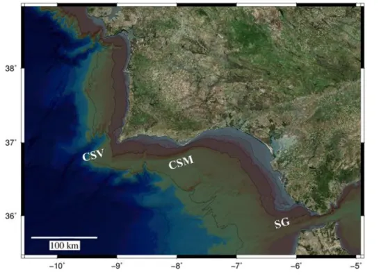
Figure 1.1- Area of interest, isobath 25m, 50m, 200m, 1000m and 2000m. Cape São Vincent
(CSV) and Cape Santa Maria (CSM), Strait Gibraltar (SG). ... 2
Figure 1.2 - Satellite SST adapted form Relvas and Barton (2005). ... 3
Figure 2.1 - ADCP location (yellow circle). ... 7
Figure 2.2 - Deployments duration, black bars indicating each deployment duration. ... 8
Figure 2.3 - ADCP Workhorse 600kHz, TRDI ... 9
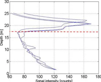
Figure 2.4 - Intensity of signal along the water column... 9
Figure 2.5 - Current velocity. Raw (red) and detide (black) using Butterworth low pass filter 40 h cut-off period. Negative values are poleward. ... 10
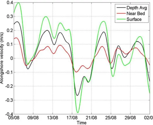
Figure 2.6 - Example of detide surface, depth average and near bed velocities. ... 11
Figure 2.7 - Peak delay scheme. Black triangles indicate peaks (first derivative =0). Near surface (green), Near bed (red). ... 12
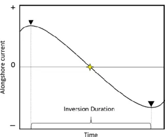
Figure 2.8 - Inversion duration scheme. Black triangles indicate peaks before and after zero-crossing (yellow star) ... 13
Figure 2.9 - Shear at zero-crossing scheme. Zero crossing in the average layer is indicated by the yellow star. Black triangles indicate the velocity values for the Near surface/bed layer where velocities differences are calculated from. ... 13
Figure 2.10 - – Slope at zero-crossing scheme. Current’s acceleration computed from the velocity variation 1hour before and 1 hour after zero-crossing (yellow star). ... 14
Figure 3.1 - Peak Delay (in hours) all data distribution ... 17
Figure 3.2 - Peak delay (in hours) seasonal distribution. Mean represented by asterisks and letters indicates groups differences obtained after Kruskall-Wallis test (P > 0.05) and Dunn post hoc comparisons. ... 18
Figure 3.3 Percentages of positive peak delay (green), peak delay > 5 hours (black), together with percentage percentages of peak delay < -5 hours (red) for each season. ... 19
Figure 3.4 - Bimonthly peak delay (in hours) distribution. Mean represented by asterisks. ... 20
Figure 3.5 - Percentages of peak delay > 5 hours(black), together with percentage percentages of peak delay < -5 hours (red) for period of two months. ... 21
Figure 3.6 - Inversion duration in hours all data distribution. Near surface left and near bed right. ... 22
VIII Figure 3.7 - Inversion duration (in hours) seasonal distribution. Near surface left and near bed right. Mean represented by asterisks ... 23 Figure 3.8 - Percentage of Inversion duration > 50 hours for each Season. Near Surface in black and near bed in red. ... 23 Figure 3.9 - Inversion duration (in hours) bimonthly distribution. Near surface left and near bed right. Mean represented by asterisks ... 24 Figure 3.10 - Percentage of Inversion duration > 50 hours for each Season. Near Surface in black and near bed in red. ... 25 Figure 3.11 - Shear at zero crossing (m/s) all data distribution. ... 26 Figure 3.12 - Shear at zero crossing (m/s) seasonal distribution. Mean represented by asterisks and letters indicates groups differences obtained after Kruskall-Wallis test (P > 0.05) and Dunn post hoc comparisons. ... 27 Figure 3.13 - Percentages of negative shear at inversion (black), together with percentage of shear >0.1 m/s (red) for each season. ... 28 Figure 3.14 - Shear at zero crossing (m/s) bimonthly distribution. Mean represented by asterisks and letters indicates groups differences obtained after Kruskall-Wallis test (P > 0.05) and Dunn post hoc comparisons. ... 29 Figure 3.15 - Percentages of negative shear at inversion (black), together with percentage of shear >0.1 m/s (red) for each period of two months. ... 30 Figure 3.16 - Slope at zero-crossing all data distribution. Near the surface layer left and near the bed layer right. ... 31 Figure 3.17 - Slope at zero-crossing (m/s2) seasonal distribution. Near surface left and near bed right. Mean represented by asterisks and letters indicates groups differences obtained after Kruskall-Wallis test (P > 0.05) and Dunn post hoc comparisons. ... 32 Figure 3.18- Seasonal percentages of High slope at zero-crossing in black and Low slope at zero crossing in red. Near the surface left and near the bed right. ... 32 Figure 3.19 - Slope at zero-crossing (m/s2) bimonthly distribution. Near surface left and near bed right. Mean represented by asterisks and letters indicates groups differences obtained after Kruskall-Wallis test (P > 0.05) and Dunn post hoc comparisons ... 33 Figure 3.20 - Bimonthly percentages of High slope at zero-crossing in black and Low slope at zero crossing in red. Near the surface left and near the bed right. ... 33 Figure 3.21- Slope differences (m/s2) all data distribution. ... 35
IX Figure 3.23 - Seasonal percentages of positive slope differences in black and high negative slope differences in red. ... 36 Figure 3.24 - Slope differences (m/s2) bimonthly distribution. ... 37 Figure 3.25 - Bimonthly percentages of positive slope differences in black and high negative slope differences in red. ... 37 Figure 3.26 - Seasonal Scatter plot of Shear at zero-crossing versus Slope at zero-crossing. Near the surface left and near the bed right. ... 38 Figure 3.27 - Shear at zero-crossing versus peak delay all data. Black letters highlight the inversion types proposed here ... 39 Figure 3.28 - Scheme for current inversion Type A, where peak delay is positive and shear at zero-crossing is negative ... 39 Figure 3.29 - Scheme for current inversion Type B, where peak delay is positive and shear at zero-crossing is positive. ... 40 Figure 3.30 - Scheme for current inversion Type C, where peak delay is negative and shear at zero-crossing is negative ... 40 Figure 3.31 - Scheme for current inversion Type D, where peak delay is negative and shear at zero-crossing is positive. ... 41 Figure 3.32 - Seasonal scatter plot of shear at zero-crossing versus peak delay. ... 41 Figure 4.1 - General model of CCCs inversions. Near the bed (red) decelerates and changes direction first. Near the surface present higher acceleration (slope) and inversion duration is very similar in both layers. ... 44 Figure 4.2 - Three-layer vertical velocity (m/s) profile. Depth average velocities (black line), Near bed (red line) and near the surface (green line). Black arrow indicates the event of 16/11/2008 to exemplify an inversion Type C. ... 45 Annex A.1- PCA applied to all parameters. Parameters loadings on the 2 maximum variance components. ... 53 Annex A.2 PCA applied to all parameters. Scores divided in seasons. ... 53
X
List of Tables
Table 2.1– Number of samples together with CCCs events for the Seasonal and bimonthly
periods defined here 15
List of Abbreviations
AH – Azores high pressure cell APG – Alongshore Pressure Gradient CCCs – Coastal Counter-Currents CSM – Cape Santa Maria
CSV – Cape Saint Vincent GC – Gulf of Cadiz SG – Strait of Gibraltar
SST – Sea Surface Temperature STD – Standard Deviation
1
1. Introduction
1.1 Motivation
At the northern margin of the Gulf of Cadiz (GC), poleward currents (from east to west in the GC) exists in turn with the coastal upwelling jets of equatorward (from west to east in the GC) direction. They are referred in the literature as “Coastal Counter-Currents” (CCCs) (Fiúza, 1983; Relvas and Barton, 2002). CCCs have been reported to be responsible for delivering warm waters within the inner shelf with a sharp temperature increase up to 3-5ºC in summer (Relvas and Barton, 2002). According to Garel et al. (2016) CCCs are a frequent feature of the inner shelf circulation (42% of the time observed), and no distinct preference for winter or summer months.
The physical drivers that control the development of CCCs in the GC remain largely speculative due to scarce long-term hydrodynamic measurements. Garel et al. (2016) stressed the need to assess the setup of CCCs at an event scale. In particular, due to the lack of detailed characterization, CCCs are treated as if they were generated by the same process, while it might not be the case.
In this sense, a more detailed and over time-assessment of the development of CCCs (i.e., at the time when the flow turns from equatorward to poleward) should contribute to the identification and understanding of the main driving forces involved.
The knowledge of CCCs - and the inner shelf circulation in general - is of interest of physical-chemical oceanography for numerical model setup and validation, to understand and predict contaminants transport. Furthermore, nutrient and planktonic organisms dispersion, are of interest for marine biology.
1.2 The Gulf of Cadiz
The GC is an embayment located between the north-western African coast and the southwestern tip of Iberian Peninsula (Figure 1.1). Its eastern boundary is defined by the Strait Gibraltar (SG) where denser waters of Mediterranean origin are exchanged and partially
2 mixed with Atlantic waters (Price et al., 1993). The westernmost limit of the GC is marked by a sharp change in the coastline direction, the Cape St. Vincent (CSV).
The region is under influence of the Azores high pressure cell (AH) and its seasonal fluctuations (Chase, 1956). In summer, the AH is stronger and the pressure gradient with Iceland low pressure cell is not pronounced, leading northern winds to blow steadily on the west coast of Iberian Peninsula creating conditions for upwelling events. Due to Ekman’s transport, surface waters are transported offshore and cold bottom waters rise in response. The Portuguese upwelling zone (Stevenson, 1977) is defined by a front of strong temperature contrast that can reach 30-50 km offshore in weak upwelling events, or 100-200 km in strong events (Fiúza, 1983).
Local features, such as the coastline discontinuity of CSV and mountains chains (Fiúza 1983; Relvas and Barton 2002; Sánchez et al., 2006), may divert the northern winds direction to westerlies in the south coast, also creating conditions for upwelling in this region. Contrarily, in winter, AH becomes weaker by its center displacement ≃10º south, culminating in gradient intensification with Iceland low. This winter set up favours winds to blow from east or southeast (Chase, 1956).
Figure 1.1- Area of interest, isobath 25m, 50m, 200m, 1000m and 2000m. Cape São Vincent (CSV) and Cape Santa Maria (CSM), Strait Gibraltar (SG).
3 1.3 Definition of coastal counter-currents
CCCs are defined as poleward flows that counter force equatorward flow generated in the western coast of Portugal.
CCCs are known to cross the entire GC northern margin (southern coastline of Portugal and Spain) and may turn clockwise around Cape São Vincent progressing up to 110 km northwards along the west coast (Relvas and Barton, 2002). In summer months, they are associated to the propagation of warm water along the southern coast (Garel et al., 2016; Relvas and Barton, 2002, 2005; Sánchez et al., 2006), while during winter this feature is not present (Garel et al., 2016).
This poleward flow occurs in a narrow band (15-20 km) restricted to the inner shelf (Criado-Aldeanueva et al., 2006; Relvas and Barton, 2005) and has the capacity to move previously upwelled waters offshore creating a high contrast temperature across the northern margin of the basin (Figure 1.2).
4 Using a multi-year (2008–2014) time-series, constituting ≃18 months of hourly records, Garel et al. (2016) found no seasonality. Poleward flows, were recorded up to 0.4 m s−1 (depth-averaged value) in accordance with Relvas and Barton, (2005). The mean duration of CCCs events were 3 days, but events lasting up to 15 days were also observed.
Local winds fail to explain the development of CCCs, although it has a clear influence on its duration and velocity. CCCs are seemingly better correlated with large-scale wind characteristic of the upwelling system (Garel et al., 2016; Sánchez et al., 2006).
Garel et al. (2016) showed that this current is mainly alongshore and barotropic. Its cross-shore component is characterized by a two-layer structure that favours transport offshore through the bottom layers, typical of downwelling conditions. While upwelled waters are typically nutrient rich, downwelling is expected to reduce nutrient availability. In fact, Navarro et al. (2006) and Rosa (2016) reported nutrient decrease coinciding with CCCs events. However, this cross-shore flow is weak, and only the long-shore velocity component is considered in the present study.
1.4 Development of CCCs
The mechanism involved in the development of CCCs in the GC largely speculative due to scarce long-term in situ hydrographic measurements. By contrast the region of Santa Barbara Channel had been the focus of extensive observations (Harms and Winant, 1998; Melton et al., 2009; Washburn et al., 2011). This region is very similar with the GC in terms of morphology and wind characteristics making it a good example for comparison. In particular, this region registers CCCs as a recurrent feature, with similar velocities of propagation at 0.46 m s−1 and a similar cross-shore behaviour (Washburn et al., 2011).
Melton et al. (2009) and Washburn et al. (2011) showed that CCCs are very well correlated to Alongshore Pressure Gradients (APG) caused by differences in sea level along the coast and to relaxation of equatorward winds. These winds opposes the APG force, when those relaxes APGs becomes the main force, triggering CCCs.
Similarly, In the GC Relvas and Barton (2002) using satellite Sea Surface Temperature images (SST), time series of sea level height (1982-1991 at four tide gauges), wind velocities, and nearshore sea surface temperature records, suggest that CCCs are driven
5 by a background APG whose effect is augmented or diminished by wind forcing. These authors also suggest that the recirculation of Atlantic waters entering the GC proposed by Mauritzen et al. (2001), can be responsible for reinforcement of the surface tilt.
Another interesting feature is the pool of warm water near Guadalquivir river mouth, present in summer SST images. Apparently, the main source of heat is land. Due to tide amplitude and negligible river discharge during spring/summer, few km2 of marsh can be flooded twice a day, and enhance energy absorption in these shallow areas. This will generate a buoyant plume of water that will contribute to the sea level slope by density effect (García-Lafuente et al., 2006).
In winter the APG is expected to diminish in relation to the seasonal change in wind conditions (Relvas and Barton, 2002); furthermore, the pool of warm water in the Gadalquivir mouth becomes a source of cold water due to the increase of fresh water discharge (Gabriel Navarro and Ruiz, 2006). Nevertheless, poleward flows are still present in winter 43% of the time (Garel et al., 2016).
It is important to note that most of these works summarized here were based on remotely sensed SST climatological data or short duration shipboard surveys. Analyses of in
situ, long-term measurements like the one performed by Garel et al. (2016) are essential to
assess the mechanisms involved on the process of generation of these currents.
1.5 Interaction with the open sea circulation
Upwelled water along the west coast causes the surface dynamic height to decrease towards the coast and consequently creating a pressure gradient with the same orientation. By geostrophic adjustment, where pressure gradient force is balanced by Coriollis effect, a flow develops in the southward direction (the so-called “upwelling jet”). Generally this flow turns eastward around CSV, but less usually, it has been observed turning westward or continuing southwards (Relvas and Barton, 2002). Water that had been upwelled in the south coast may merge into the jet that turned around the cape and deliver cold waters into the GC basin (Sanchez and Relvas, 2003).
Several studies have reported a quasi-permanent cyclonic circulation in the central part of GC (Criado-Aldeanueva et al., 2009; García-Lafuente et al., 2006; Garcia et al., 2002;
6 Sanchez and Relvas, 2003). Vargas et al. (2002) performed an Empirical Orthogonal Function analysis to identified spatial patterns of satellite SST images in the GC. They also observed a frequent warm region in the southern part of the area of study.
In winter, the cyclonic eddy becomes weaker and displaces southward. This eddy is thought to act as a connection of the jet of upwelled waters with the SG (Peliz et al., 2009; Peliz et al., 2007).
Mauritzen et al. (2001) states that recirculation is required in the northern margin of GC due to the excess of Atlantic waters entering the SG. The excessed water that is not needed to enter the strait, gains salinity from the underlying Mediterranean outflow and flows poleward over the continental shelf.
García-Lafuente et al. (2006) defined the circulation of the inner shelf in the GC composed by two cyclonic gyres that can be connected when wind conditions are favourable: The first gyre, located in the eastern side, is a result of the geostrophic adjustment due to the density gradient created by the equatorward cold jet and warmer waters of the inner shelf. The cyclonic circulation becomes complete when this current is forced to turn south-westwards (partially at least) and merge again within the equatorward flow due to the presence of Cape Santa Maria. The second gyre, located in the western part, seems to be related to the response of wind stress in the region of CSV (Mazé et al., 1997). A more recent work of Relvas and Barton (2005) identified the same structure flow and justified, using computed surface dynamic heights, that it was a surface signature of a deeper Mediterranean water eddy (i.e. Meddies).
1.6 Objectives
In order to categorize CCCs setup (i.e., “inversions”, defined hereafter strictly as the moment of maximum acceleration in the equatorward direction preceding the flow direction change until the moment of maximum acceleration in the poleward direction), and bring more evidence on their controlling mechanisms, multi-year current data were collected with a bottom-mounted Acoustic Doppler Current Profilers (ADCP), between 2008 and 2017, in the south Portuguese inner shelf.
7 The main goal of the present research is to exploit this dataset in order to characterize the variability of inversion patterns (and thus identifying various types of CCCs) by performing a detailed analysis of the along-shore flow structure during these events. Important to be mentioned, the reversal phenomena (defined here as the turn of the flow from poleward to equatorward) behaviour is not under the scope of this study. Inversion types were inferred by the mutual analysis of several parameters extracted from inversions. It is further proposed to explore if the identified types of inversion reflect the action of potential responsible forces for the development of these currents.
2. Materials and methods
2.1 Data
The time-series used to reach the proposed objective are composed by a multi-year curent velocity recorded at Armona station (37°0,648′ N; 7°44,480′ W) at 23m depth (Figure 2.1), using a Workhorse 600kHz, TRDI ADCP bottom mounted on top of a concrete artificial reef of 1.4 m height.
8 A total of 13 deployments were performed at different times of the year (Figure 2.2),
and 22153 samples were recorded.
From 2008 until 2017, the years of 2009, 2011 and 2012 were not sampled while 2008, 2014 and 2015 were the years with more samples.
It is clear that the second half of the year present a higher sampling coverage and thus results must had been analysed carefully considering the coverage patterns, especially when considering the month of March.
The ADCP device (Figure. 2.3) is used to record water flow velocity in three dimensions, near bed temperature and pressure. Two independent sensors measure temperature and pressure. Velocity is measured by emitting an acoustic signal that is reflected by particles present in the water. By receiving back, the signal, and verifying the frequency changes it suffers from the reflection, the velocity of the particles can be calculated (Doppler effect). This velocity is considered as equal to the flow velocity. The equipment has an internal compass and data are recorded in orientation of N-S W-E Cartesian coordinates. Velocities are recorded at different depths (cells) along the water column. The width of each cell is dependent of the set up used for each deployment.
9 Data were recorded at hourly
intervals, along cell sizes of 0.5 m, (except for deplymnent of October-December in 2008 where the cell size was 1 m).
2.2 Data processing
Once the data had not been through any processing, the first task to be accomplished was the preparation of the time-series for their analysis.
The processing of the data was performed by Matlab (v.2014) script that consisted of:
1- Remove cells with invalid data (out of water or contaminated by the surface boundary) – The number of valid cells can vary due tide, waves or particles and needed to be corrected. The criteria used for removing invalid cells was the signal intensity. When signal suffer a sharp increase in intensity (due to the influence of the water surface) cells above this level were discarded. Figure 2.4 exemplifies a set of measurements where blue lines represent
Figure 2.3 - ADCP Workhorse 600kHz, TRDI
10 the signal intensity and dashed red line highlight the threshold mentioned above. In this case, cells above 17 m were flagged as invalid. Validated cells data were rotated in cross-shore and along-shore components using the angle of maximum variance (22.9º). A simple linear regression using the raw velocities showed the angle of maximum variance. Positive alongshore current velocities represent W-E direction and negative, E-W.
3- Remove tidal signal from current records – The tidal cycle is semi-diurnal in the region, and therefore every 12 hours 25 min a cycle is complete. These oscillations have an effect in the horizontal movement of the water and have to be removed using a Butterworth low-pass filter using a 40 hours cut-off period. An example is presented in Figure 2.5.
4- Extract the near surface, depth average and near bed layer velocities from the detide time series (Figure 2.6).
Near surface was defined to be the mean value of the 2 uppermost valid cells. Averaging is done to reduce the standard deviation (i.e., small errors affecting measurements
Figure 2.5 - Current velocity. Raw (red) and detide (black) using Butterworth low pass filter 40 h cut-off period. Negative values are poleward.
11 at each cell). Depth average was defined to be the mean of all cells and near bed was the mean of the 2 cells closest to the bottom.
Data was compiled in a catalogue based in all the ADCP data available. It was built on the definition of parameters defined here (see next section) applied for the three water layers (near surface, depth average and near bed).
The construction of the catalogue allowed to group all identified inversions and their parameters and further the creation of inversion categories by assessing the distribution of parameters.
2.3 Parameters definition
Peak delay - A peak is defined here, as the closest significant peak before and after direction change. It is chosen when the first derivative of the velocity signal is zero. It is the
12 point of maximum velocity preceding and after signal zero-crossing. Between these points, it is assumed that the driving forces of inversions are predominant.
Peak delay is measured in hours, this parameter quantifies time interval between peaks of surface and bed layers before inversion (Figure 2.7). Positive values indicate that near bed layer started to turn (decelerate) before the near surface layer. Negative values represent the opposite, near surface layer started to turn before near bed layer.
For few cases, the selection of the peak delay was a complicated task, and peaks could have been chosen differently. A specific peak (first derivative of the velocity signal equals zero), could have been preceded by another peak where the velocity signal was greater making the selection of the peak difficult. However, doubtful peak selection was not a recurrent situation and main results would not suffer critical changes.
Inversion Duration - Time interval in hours between the peaks before and after zero-crossing. It measures the time interval of when the velocity started to decrease in the equatorward direction until it stopped to accelerate in the poleward direction (Figure 2.8). This parameter was measured for near surface and near bed layers.
Figure 2.7 - Peak delay scheme. Black triangles indicate peaks (first derivative =0). Near surface (green), Near bed (red).
13 Shear at zero-crossing – Shear is calculated from the velocity differences between the near surface layer and the near bed (surface minus bed) at the time when the average velocity changes signal (Figure 2.9). Positive values of shear indicate that the near bed layer inverted before the near surface layer and negative values indicates the opposite, near surface changes direction before the bed.
Figure 2.8 - Inversion duration scheme. Black triangles indicate peaks before and after zero-crossing (yellow star)
Figure 2.9 - Shear at zero-crossing scheme. Zero crossing in the average layer is indicated by the yellow star. Black triangles indicate the velocity values for the Near surface/bed layer where velocities differences are calculated from.
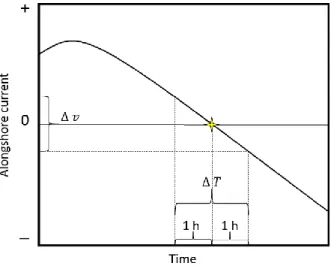
14 Slope at zero-crossing (Δv/ΔT) – Velocity slope computed from points 1 hour before and after the inversion in the different layers: near surface and near bed (Figure 2.10). It quantifies the acceleration of current.
Slope will be assessed using the definition of high slope and low slope. It is defined here as the mean value ± standard deviation (STD) of all data distribution for each layer.
Slope differences – Slope at zero-crossing differences between near surface and near bed layers (surface minus bed). Positive values of Slope differences mean that near bed layer has a higher acceleration than near surface, and negative values the opposite, near surface layer has a higher acceleration than near bed.
Some cases where slope differences resulted in a positive value, were also recorded in a doubtful situation. Sometimes, the moment of direction change of surface layer, was very close to the velocity maximum or close to a short velocity deceleration-acceleration moment. In both situations slope at zero crossing becomes close to zero, even though the total inversion slope is more accentuated. This few cases resulted in the most extreme positive values presented here (>1x10⁻⁶). Again, these specific cases do not affect the main findings of the
slope related parameters.
Slope differences will be assessed using the definition of positive and high negative slope differences, defined here as mean minus STD.
Figure 2.10 - – Slope at zero-crossing scheme. Current’s acceleration computed from the velocity variation 1hour before and 1 hour after zero-crossing (yellow star).
15 2.4 Temporal periods and seasonal definition
The data were sampled during different periods over several years, and therefore, the analysis will be performed using different periods to verify any variability in the dataset. Firstly, each parameter will be analysed considering all the data. Secondly, variability will be checked seasonally and at last using bimonthly time scales.
Seasonal variations were analysed considering the typical seasons in the region, i.e. winter (from December until February), spring (from March until May), summer (from June until August) and Autumn (from September until November). Bimonthly variations were analysed by selecting groups of two months as: January – February, March – April, May – June, July - August, September - October, November – December. These groups were selected since some of these months present similarities that could be hidden in the seasonal analysis. For example, the characteristics of the month of June, in some parameters, are closer to May than to August, although it belongs to the summer season.
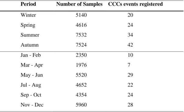
The Seasonal periods defined here, present comparable number of samples and number of CCCs registered events for most of the periods (Table 2.1). For the bimonthly analysis, the number of samples of the March-April period should be assessed carefully, as it presents only 1976 samples and 7 CCCs events.
Table 2.1– Number of samples together with CCCs events for the Seasonal and bimonthly periods defined here.
Period Number of Samples CCCs events registered
Winter 5140 20 Spring 4616 24 Summer 7532 34 Autumn 7524 42 Jan - Feb 2350 10 Mar - Apr 1976 7 May - Jun 5520 29 Jul - Aug 4652 22 Sep - Oct 4354 24 Nov - Dec 5960 28
16 2.5 Statistical and parameters integrative analysis
Parameters distribution were analysed using a boxplot representation. The main information used for the analysis was regarding the mean value, the STD and the interquartile range (IQR). Extreme values were not considered outliers, they rather represent extreme events.
Normality (Kolmogorov–Smirnov test) and homogeneity of variances (Levene’s test) were verified prior to statistical comparisons among seasons and bimonthly periods.
To identify if seasons and bimonthly periods come from an identically distributed population, the performed comparisons were based on the non-parametric Kruskal-Wallis test, and on a non-parametric Dunn post-hoc multiple comparisons (Dunn, 1964).
The best relationship observed among parameters was obtained visually using scatter plots of Peak delay and Shear at zero-crossing. Inversions types were created considering the sign of the parameters, and all 4-possible combination generated the 4 types proposed.
A multivariate analysis (Principal Component Analysis – PCA) was performed using the software STATISTICA 8.0, in order to integrate the relevant parameters and assess their potential seasonal correlation. Results obtained using this technique showed no meaningful variance of parameters in relation to seasons (see annex A).
3.
Results
3.1 Data overview
The analysis of the data-series allowed the observation of 120 current inversions during the 13 deployments performed (≃9 inversions per deployment in average).
In the poleward direction, velocity can reach up to 0.41 m/s in the average layer, the mean peak velocity is 0.17 m/s. Near the surface CCCs maximum is 0.65 m/s and mean peak velocity equals to 0.21 m/s. Near the bed velocity can reach up to 0.27 m/s with the mean peak velocity reaching 0.09 m/s. CCCs events can have one or more velocity peak during its duration. On average, a CCCs event, develop 1.5 peaks
17 CCCs events occurs in average 3.35 times per month. The longest CCCs registered last for 534 hours (≃22 days) on the 15th of October until the 6th of November in 2015.
3.2 Parameters results 3.2.1 Peak delay
The Peak delay distribution represented in Figure 3.1, shows that positive peak delay, where near bed layer started to turn before the near surface layer occur more often 79%, against 21% of negative peak delay where near surface started to turn before the bed layer. For most of the cases (60.8%) the delay is less than 5 hours, 44.2% occur from 0 to 5 hours and 16.7% occur from 0 to -5 hours.
Peak delay can range from ≃-15 hours to ≃27 hours and the mean value is 3.65 hours with STD equals to 6.13 hours. Positive peak delay is on average 5.6 hours with 4.97 hours STD and negative peak delay is on average -3.73 hours with STD 4.24 hours.
18 3.2.1.1 Seasons
Along the year the mean value of peak delay is highest in spring and decreases towards winter together with the variability of the data. Note that the IQR in winter is approximately the half of spring (Figure 3.2). In winter peak delay is 0.26 hours on average with STD 3.86 hours, in spring 5.88 hours (STD 7.19 hours), in summer 4.6 hours (STD 5.11 hours), in autumn 3.22 hours (STD 6.54 hours).
During winter, extreme values are not registered as it is in the other seasons, 85% of the cases peak delay is within the range of -5 to 5 hours.
Seasons showed statistically significant differences among themselves (Kruskall-Wallis test P > 0.05) and the post hoc test indicated that winter differs more from spring and summer while autumn is a transitory period.
Figure 3.2 - Peak delay (in hours) seasonal distribution. Mean represented by asterisks and letters indicates groups differences obtained after Kruskall-Wallis test (P > 0.05) and Dunn post hoc comparisons.
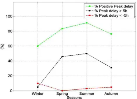
19 Winter present the lowest percentage of positive peak delay (60%). While spring present 83 %, summer 91% and autumn 76% (Figure 3.3).
Peak delay > 5hours happens with more frequency in the summer months (50%) and seldom registered in winter (5%). Peak delay <-5 hours have much less expression, it is absent in spring, 3% in summer, 5% in autumn and its maximum occurs in winter (10%).
3.2.1.2 Bimonthly scale analysis
When peak delay distribution is plotted in function of two months period (Figure 3.4) the seasonal fluctuation of the mean values maintains, with higher values in spring-summer and lower in winter-autumn months.
The mean value for all periods of two months is positive except for the period of January-February (mean -0.16 hours and STD 3.83 hours). Mean is highest for the period of March-April (6.90 hours and 9.96 STD hours), for this period the variability is also the largest
Figure 3.3 Percentages of positive peak delay (green), peak delay > 5 hours (black), together with percentage percentages of peak delay < -5 hours (red) for each season.
20 (wider IQR). During May-June mean peak delay is 5.06 hours, in July-August 4.65 hours, in September-October 3.79 hours and finally November-December with a mean value (1.82 hours) and distribution similar to January-February.
Although the Kruskall-Wallis test presented a value of P < 0.05 the post hoc test did not show significant differences among the bimonthly periods.
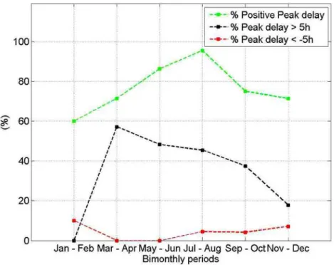
The percentage of positive peak delay is the highest in July-August (95.5%), while the lowest (40%) is registered in the period of January-February (Figure 3.5). The period of March-April present 57% of peak delay >5 hours while the period of January-February presents the highest percentages of peak delay <-5 hours (10%).
21 3.2.1.3 Summary of main observations
Peak delay analysis showed that inversions begin near the bed first, and occurs more from March to August. The period of March-April presents the highest percentages of extreme positive values of peak delay.
Negative peak delay may occur any time with relatively low frequency. It is more present from November to February, but the few extreme negative values appeared between July and December.
The analysis of this parameter highlighted that there is a strong difference in the development of the inversion between winter and spring-summer.
3.2.2 Inversion Duration
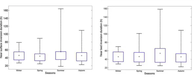
The Inversion duration is on average, 48.25 hours (STD 23.56 hours) in the surface layer and 48.41 hours (STD 23.1 hours) near the bed. Most of the inversions are comprised
Figure 3.5 - Percentages of peak delay > 5 hours(black), together with percentage percentages of peak delay < -5 hours (red) for period of two months.
22 between 20 and 50 hours as shown in figure 3.6. Near the surface 70% of the registered inversions, last less than 50 hours and near the bed 67.5%.
Both layers distributions are very similar even on their range. Near the surface inversions range from 18.43 hours up to 164.08 hours. Near the bed it ranges from 22.22 hours to 158.75 hours. For the same event of CCCs, near surface and near bed layers can present durations that can differ up to 40-50 hours one from another. These situations were rather rare and in general differences on inversion duration between layers were small.
No statistically significant differences (Kruskall-Wallis test P > 0.05) were found in the seasonal neither in the bimonthly scale analysis of inversion duration for both layers.
3.2.2.1 Seasons
Figure 3.7 represent the inversion duration distribution in function of seasons. For both layers the summer period is when the mean values of inversion duration are the highest, 55.36 hours near surface and 54.26 hours near bed approximately, 10 hours more than the other seasons. For the same period variability also increases in both layers presenting highest STD values, 34.4 and 32 hours for near the surface and near the bed layers respectively.
23 Figure 3.8 shows the variation on the percentage of inversion duration >50 hours and highlight the difference between the two layers. In winter it was registered 40 % near bed against 30 % near surface.
Figure 3.7 - Inversion duration (in hours) seasonal distribution. Near surface left and near bed right. Mean represented by asterisks
Figure 3.8 - Percentage of Inversion duration > 50 hours for each Season. Near Surface in black and near bed in red.
24 3.2.2.2 Bimonthly scale analysis
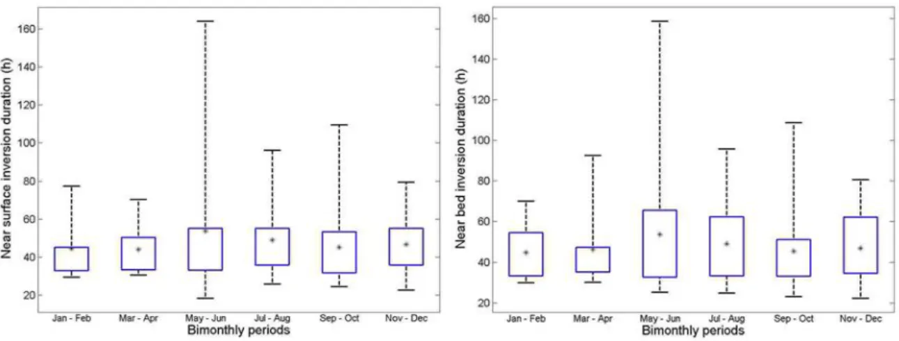
The bimonthly distribution of Inversion duration presented in Figure 3.9 shows that the highest mean values were registered in the period of May-June in both layers. Near surface the mean value reach 53.79 hours and 53.68 hours near the bed.
From July to December, inversion duration mean value and distribution do not vary much. From January to April inversion duration data tend to present lower variability values with small IQR.
The occurrence of long inversions (>50 hours) is more frequent in the period of November-December (Figure 3.10). Near the surface this period present 35.71% of long inversions and near bed 39.29%
Figure 3.9 - Inversion duration (in hours) bimonthly distribution. Near surface left and near bed right. Mean represented by asterisks
25 3.2.2.3 Summary of main observations
Current inversions duration is on average, two days in both layers. Inversion duration distribution is very similar among layers and no strong difference is observed between layers along the year.
In general inversions are shorter in winter months. From May to December inversion duration is more variable and generally longer.
3.2.3 Shear at zero-crossing
Values of Shear vary from -0.05 m/s to 0.16 m/s (Figure 3.11). The mean shear value is 0.05 m/s with STD 0.05 m/s. Positive and negative Shear occurs 77% and 23% of the time respectively.
Figure 3.10 - Percentage of Inversion duration > 50 hours for each Season. Near Surface in black and near bed in red.
26 The distribution seems to present two populations, the first ranging from -0.05 m/s up to 0.1 m/s representing 78 % and the other from 0.1 m/s up the 0.16 m/s that represent 22%
of the total distribution.
3.2.3.1 Seasons
When Shear is plotted with seasonality (Figure 3.12), winter presents low values of shear, the mean is the lowest among seasons (0.02 m/s). In spring mean increases to 0.07 m/s and in summer 0.06 m/s. In autumn, the distribution is similar to summer with a slight decrease of the mean to 0.04 m/s, due to the presence of more negative shear.
Data variability are different among seasons, winter present the lowest STD (0.04 m/s) while summer the highest (0.06 m/s). STD values does not stand out much the differences among seasons, IQR shows the same relation but with differences more evidenced (0.04 m/s for winter and 0.1 m/s for summer).
Kruskall-Wallis test showed that seasons present statistically significant differences (P < 0,05) and the post hoc comparisons indicates that spring and winter have the strong differences and a difference between spring and autumn is also observed.
27 In Figure 3.13 is represented the percentage of negative shear for each season together with the fluctuations of the percentages of shear >0.1 m/s. Winter present 30% of negative shear and percentage of shear >0.1 m/s is the lowest (5%). Spring present inversions with preference to have positive shear, negative shear represent only 8%. For this period, the percentage of shear >0.1 m/s is 21%. In summer 12% of the cases present positive shear and the percentage of shear >0.1 m/s increases to 32%. In autumn, the presence of negative shear is the highest (36%) and the percentage of shear >0.1 m/s decreases to 21%.
Figure 3.12 - Shear at zero crossing (m/s) seasonal distribution. Mean represented by asterisks and letters indicates groups differences obtained after Kruskall-Wallis test (P > 0.05) and Dunn post hoc comparisons.
28 3.2.3.2 Bimonthly scale analysis
The small-scale analysis of the Shear at inversion in Figure 3.14 shows that for the period between January-February, there is a high number of shear with low values (interquartile range from -0.001 m/s to 0.025 m/s), the lowest mean value (0.01 m/s) and STD is also the smallest (0.02).
For the period of March-April the mean is the highest (0.08 m/s) and decreases toward September- October 0.03 m/s. Note that for this period the lower quartile is the lowest (-0.02 m/s) and the IQR encompass more negative values.
The post hoc test for the seasonal analysis showed winter and spring as the periods with the most significant statistical differences, followed by spring and autumn differences. The bimonthly analysis showed that the periods of May-June and September-October as those with the main differences, and the group of two months that belongs to the winter-spring periods present more of a transitory behaviour.
Figure 3.13 - Percentages of negative shear at inversion (black), together with percentage of shear >0.1 m/s (red) for each season.
29 In Figure 3.15 is possible to assess the weight of negative shear together with shear > 0.1 m/s for each bimonthly period. In the January-February period, negative shear represents 40% of the cases and no shear >0.1 m/s is observed. March-April also present no negative shear but shear >0.1 m/s represents 29%. The period of May-June, in 5 % of the cases shear is negative and 30% is >0.1 m/s. In July-August 18% of the cases, shear is positive and 27% is >0.01 m/s. In September-October, the percentage of negative shear reach 46%. Shear with values >0.01 m/s happens 17% of the time. For November-December, the positive-negative ratio is 79% and 21% respectively with 21% of shear >0.1 m/s.
Figure 3.14 - Shear at zero crossing (m/s) bimonthly distribution. Mean represented by asterisks and letters indicates groups differences obtained after Kruskall-Wallis test (P > 0.05) and Dunn post hoc comparisons.
30 3.2.3.3 Summary of main observations
Shear at zero-crossing analysis indicates that the counter-currents tends to start near the bottom most of the times. Values of positive shear can reach 0.16 m/s which is an order of magnitude larger than the maximum negative shear -0.05 m/s.
Along the year the main differences on Shear values showed to be between the late spring time, against early autumn.
Interestingly shear values has a broad range from March until December, but the transition to January-February period is very abrupt. On average shear is weak and less variable during winter (preferably in January and February). Extreme values happen in the other seasons. The period of March until August has the most positive shear values while September and October is more likely to occur both situations and with a highest percentage of negative shear.
Figure 3.15 - Percentages of negative shear at inversion (black), together with percentage of shear >0.1 m/s (red) for each period of two months.
31 3.2.4 Slope at zero-crossing
Slope distribution (Figure 3.16) shows that near bed inversions occur with a much lower acceleration than near surface. Note that slope increase with negative values. Mean value and minimum near surface are approximately double of the near bed. Near surface present a mean value of -0.4x10⁻⁵ m/s2 with STD 2.25x10⁻⁶ m/s2 and minimum of -1x10⁻⁵ m/s2. Near bed mean value is -0.17x10⁻⁵ m/s2 with STD 0.8x10⁻⁶ m/s2 and the minimum reach -0.4x 10⁻⁵ m/s2. For both layers when slope is less accentuated it is around 0.2x 10⁻⁶ m/s2.
As described in the parameters definition Slope will be also assessed in terms of high and low slope. Near the surface, high slope (mean minus STD) is <=-0.6x10⁻⁵ m/s2 and
represents 18%. Low slope (mean plus STD) is >=-0.17x10⁻⁵ m/s2 and represent 17%.
3.2.4.1 Seasons
In the surface layer Slope values does not oscillate much along the year. Generally, both layer present similar trend, higher slope in winter-spring and lower slope in summer-autumn (Figure 3.17).
Kruskall-Wallis test showed significant statically differences (P > 0.05) only for the near bed Slope at zero-crossing. The post hoc comparisons indicated that summer and autumn are distinct from winter and spring as being a transitory period.
32 Figure 3.18 confirm the tendency of decreasing slope towards autumn as the frequency of low slope increases from winter to autumn. Near the surface the frequency of high slope do not fluctuate along the year, while near the bed high slope has its maximum in winter 40% and minimum in autumn 10%.
3.2.4.2 Bimonthly scale analysis
When Slope at zero-crossing is plotted in function of two months period (Figure 3.19) the tendency of decreasing slope towards autumn disappear and fluctuations of the mean values are not marked. Again, the Kruskall-Wallis test showed significant statically
Figure 3.17 - Slope at zero-crossing (m/s2) seasonal distribution. Near surface left and near bed right. Mean
represented by asterisks and letters indicates groups differences obtained after Kruskall-Wallis test (P > 0.05) and Dunn post hoc comparisons.
Figure 3.18- Seasonal percentages of High slope at zero-crossing in black and Low slope at zero crossing in red. Near the surface left and near the bed right.
33 differences (P > 0.05) only for the near bed Slope at zero-crossing. The periods flagged as different by the post hoc comparison was the period of September-October against November-December. Note that the period of September-October presents the lowest mean 1.7x10⁻⁶ m/s2 and one of the lowest IQR 6.6x10⁻⁶ m/s2 and November-October the Highest
mean 2x10⁻⁶ m/s2.
The fluctuation of high slope near the bed is not so marked (Figure 3.20), but as in the seasonal analysis, during winter months is when high slopes are more present.
Near the surface, the percentage of low slope reach the maximum in the period from September until December (25%). Near the bed only the period of September-October presents a sharp increase on the low slope frequency that reaches 33%, 3 times more than the previous period July-August with 9%.
Figure 3.19 - Slope at zero-crossing (m/s2) bimonthly distribution. Near surface left and near bed right. Mean
represented by asterisks and letters indicates groups differences obtained after Kruskall-Wallis test (P > 0.05) and Dunn post hoc comparisons
Figure 3.20 - Bimonthly percentages of High slope at zero-crossing in black and Low slope at zero crossing in red. Near the surface left and near the bed right.
34 3.2.4.3 Summary of main observations
Along the year, slope at zero-crossing does not present strong fluctuations near the surface.
Near the bed generally, winter Current inversion occur with a higher acceleration and in autumn the opposite. The increase on the percentage of low slope towards autumn is what suggests the deceleration on the current inversion. The period of September and October is where the most pronounced change is observed.
3.2.5 Slope Differences
Figure 3.21 represents the whole data distribution for Slope at zero-crossing differences (Slope near surface minus slope near bed). When slope differences are positive it means that near the bed layer had a more accentuated slope than near the surface. As described above, near bed slope is generally weaker than near surface, this way, Slope differences is majority negative occurring 90% of the time recorded. For the 10% of positive slope differences values are much lower than the opposite situation the mean of all positive values of slope differences is 0.7x10⁻⁶ m/s2.
The differences range between -8.3x10⁻⁶ m/s2 and 1.9x10⁻⁶ m/s2. The mean value is 2.22x10⁻⁶ m/s2 (STD 1.9x10⁻⁶ m/s2). As described in the parameters definition the Slope differences will be also assessed in terms of high negative slope differences (mean minus STD). For the whole data set it represent 16% of the cases.
35 3.2.5.1 Seasons
Seasonal distribution of Slope differences in Figure 3.22 shows that in autumn is when the mean value is the closest to zero -1.80x10⁻⁶ m/s2 and STD 1.95x10⁻⁶ m/s2 and both layers tend to invert with similar acceleration. In summer, the variability is increased. This
Figure 3.22 - Slope differences (m/s2) seasonal distribution. Mean
represented by asterisks.
36 period presents the highest STD 2.4x10⁻⁶ m/s2 and the highest IQR 3.1x10⁻⁶ m/s2.
The main feature in the seasonal distribution of Slope differences is that, in the summer period, values present a broader range. In fact, summer present both the highest percentages of positive slope differences (15%) and the highest percentage of high negative slope differences (21%). In the other hand winter period present the lowest percentages of both extreme values (Figure 3.23).
3.2.5.2 Bimonthly time scale analysis
When Slope differences distribution is plotted in the bimonthly time scale (Figure 3.24), it is observed that the mean values do not fluctuate significantly. Data variability for the period of January-February is the lowest. IQR is equal to 6.6x10⁻⁷ m/s2, one order of magnitude lower than the other periods.
Figure 3.23 - Seasonal percentages of positive slope differences in black and high negative slope differences in red.
37 Figure 3.25 shows that high negative slope differences may happen all year but not in January-February. There is a peak on the percentage of high negative slope differences for the period of March-April.
Figure 3.24 - Slope differences (m/s2) bimonthly distribution.
Figure 3.25 - Bimonthly percentages of positive slope differences in black and high negative slope differences in red.
38 Positive Slope differences also follows the same trend, it appears with low frequency (maximum 14% for the period of November and December) from May until December.
3.2.5.3 Summary of main observations
During the first two months of the year, both layers invert with minimum slope differences. For the time recorded, near surface had always a higher acceleration with only 12 events where near bed had higher acceleration and when it happened the difference was very low.
3.3 Parameters integrative analysis
To first assess the relationship between parameters, scatter plots were created, and no strong correlation was found in most of the cases. In Figure 3.26 where Shear at zero-crossing is plotted against Slope at zero-crossing there is an indication of inverse correlation for the surface layer during spring (Figure 3.26 left). The same pattern is not observed near the bed as the slope is a parameter with very low fluctuations for this layer.
Figure 3.26 - Seasonal Scatter plot of Shear at zero-crossing versus Slope at zero-crossing. Near the surface left and near the bed right.
39 In Figure 3.27 the scatter of Shear at zero-crossing versus peak delay highlight and summarize the types of inversion that can occur.
Type A – occurs 16.7% of the observed time. CCC Type A, starts to turn near the bed and when the average layer crosses zero, near surface had already changed sign while near bed is still equatorward (Figure 3.28).
Figure 3.28 - Scheme for current inversion Type A, where peak delay is positive and shear at zero-crossing is negative
Figure 3.27 - Shear at zero-crossing versus peak delay all data. Black letters highlight the inversion types proposed here
40 Type B – is the most common type (62.5%). CCC Type B, starts to turn near the bed and when the average layer crosses zero, near bed had changed sign and near surface is still
equatorward (Figure 3.29).
Type C – is a rare case and occurs only 5.8% of the time. Inversions Type C starts to turn near the surface and when the average layer crosses zero, near surface had already changed sign while near bed is still equatorward (Figure 3.30).
Figure 3.29 - Scheme for current inversion Type B, where peak delay is positive and shear at zero-crossing is positive.
Figure 3.30 - Scheme for current inversion Type C, where peak delay is negative and shear at zero-crossing is negative
41 Type D – Inversions type D starts to turn near the surface and when the average layer crosses zero, near bed had changed sign and near surface is still equatorward. It happens 15% of the time (Figure 3.31).
When these 4 different types of inversions are plot seasonally (Figure 3.32) it gains more shape and it is possible to track when a specific type occurs more preferably.
Figure 3.31 - Scheme for current inversion Type D, where peak delay is negative and shear at zero-crossing is positive.
Figure 3.32 - Seasonal scatter plot of shear at zero-crossing versus peak delay.
A B D C A B C D D A C B B D A C