Diffusion kurtosis imaging of the healthy human brain

(1)

Universidade de Lisboa

Faculdade de Ciência

Departamento de Física

Diffusion Kurtosis Imaging of the Healthy

Human Brain

Rafael Neto Henriques

Dissertação

Mestrado Integrado em Engenharia Biomédica e Biofísica

Perfil em Radiações em Diagnóstico e Terapia

(2)

(3)

Universidade de Lisboa

Faculdade de Ciência

Departamento de Física

Diffusion Kurtosis Imaging of the Healthy

Human Brain

Rafael Neto Henriques

Dissertação

Mestrado Integrado em Engenharia Biomédica e Biofísica

Perfil em Radiações em Diagnóstico e Terapia

Orientadores:

Doutora Marta Morgado Correia

Professor Doutor Hugo Alexandre Ferreira

(4)

(5)

V

Resumo

Nas últimas décadas, a esperança média de vida tem vindo a aumentar. Desta forma, é cada vez mais importante perceber como se pode providenciar um envelhecimento saudável. Apesar de ser comum relacionar o envelhecimento com a perda de capacidades cognitivas, estudos recentes sugerem que certas capacidades cognitivas podem ser preservadas, ou mesmo melhoradas, uma vez que o cérebro pode manter-se flexível ao longo dos anos. O projecto „Cambridge Centre for Ageing and Neuroscience‟ (Cam-CAN) é um projecto colaborativo que tem como objectivo determinar o grau de flexibilidade neural ao longo da vida e o potencial de reorganização neuronal para a sustentação das capacidades cognitivas. Esse conhecimento será importante para compreender como podemos preservar os recursos cognitivos e aumentar a qualidade de vida. Deste modo, pretende-se analisar dados demográficos, psicológicos, físicos e neuronais de 700 participantes com idades compreendidas entre os 18 e os 90 anos. Relativamente aos dados neuronais, este projecto inclui dados obtidos por magnetoencefalografia e por ressonância magnética estrutural, funcional e por difusão.

Desde a década de oitenta, as técnicas de ressonância magnética por difusão têm mostrado grande utilidade em várias aplicações. Como os processos de difusão dependem das características microscópicas dos tecidos, a ressonância magnética por difusão pode revelar alterações microscópicas na resolução normal das imagens de ressonância magnética. Em 1994, Basser, Mattiello e Lebihan introduziram uma nova perspectiva nas medidas de difusão para tecidos anisotrópicos, como é o caso da matéria branca do cérebro. Conhecida por imagem por tensor de difusão ou diffusion tensor

imaging (DTI), esta técnica caracteriza os processos de difusão por tensores em vez de

um único escalar. Contudo, a DTI baseia-se na hipótese que a difusão de moléculas de água pode ser caracterizada por uma distribuição Gaussiana, o que foi demonstrado não ser completamente adequado. Em particular, foi observado que as barreiras das microestruturas tecidulares introduzem desvios simétricos relativamente à distribuição Gaussiana. Imagem por curtose de difusão ou diffusion kurtosis imaging (DKI) é uma expansão da DTI, onde o tensor de difusão é estimado em conjunto com o tensor de curtose que caracteriza o grau de não-gaussianidade de difusão em meios anisotrópicos. Esta técnica proporciona melhores estimativas dos parâmetros de difusão comparativamente à DTI, obtendo-se um índice de complexidade das barreiras dos

(6)

VI

tecidos. Por exemplo, a partir dos tensores de difusão e curtoses podem ser obtidos: 1) os valores da difusão e curtoses na direcção paralela às fibras de matéria branca (λ∥ e k∥); 2)

os valores médios da difusão e curtoses nas direcções perpendiculares às fibras de matéria branca (λ⊥ e k⊥); 3) os valores médios de difusão e curtoses em todas as orientações espaciais (MD e MK); e 4) um índice de anisotropia do tensor de difusão (FA). Tal como qualquer técnica de ressonância magnética, a DKI está sujeita a ruído e a artefactos, o que pode levar a valores implausíveis de difusão e curtoses. Desta forma, é importante desenvolver métodos mais robustos para o processamento e análise da DKI.

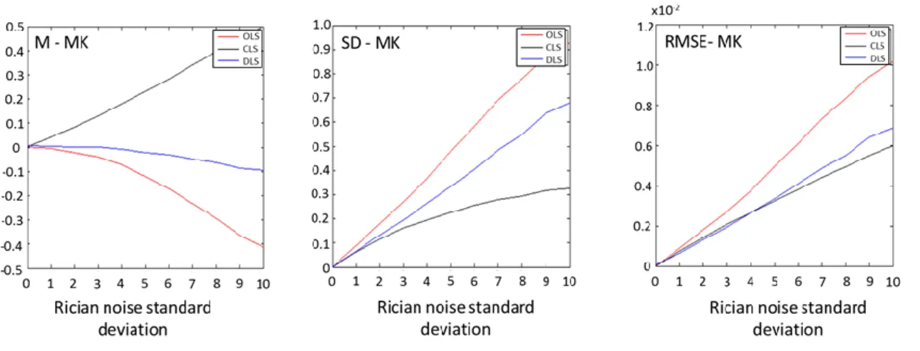
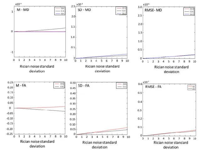
O trabalho desta tese teve como objectivo melhorar os dados da DKI extraidos dos dados de difusão do Cam-CAN (que correspondem a 63 volumes de imagens para cada sujeito: 30 direcções para b-values = 1000, 2000 s.mm-2 e 3 b-value=0 s.mm-2). Para tal, foram testados diferentes algoritmos para a estimativa dos tensores de difusão e curtoses em dados de ressonância magnética por difusão simulados e corrompidos por ruído Riciano artificial. Os diferentes algoritmos incluíram: 1) uma solução simples obtida pela minimização do modelo da DKI pelos métodos dos mínimos quadrados (OLS); 2) uma solução mais geral obtida pela minimização dos mínimos quadrados onde uma estimativa da variância dos pontos é inserida para corrigir a não homocedasticidade dos dados (WLS); 3) um método iterativo não linear (NLS); 4) um método iterativo não linear em que o tensor de difusão é escrito pela decomposição de Choslesky para forçar estimativas plausíveis de difusão (chNLS); 5) um método iterativo linear em que restrições são introduzidas para impedir que valores de difusão e curtoses sejam estimados por valores implausíveis (CLS); e 6) um novo método proposto para a estimação directa dos valores de MD e MK (DLS). Dois tipos de simulações foram testados: simulações baseadas em tensores para um único voxel de matéria branca e baseados em tensores correspondentes a um cérebro inteiro. Para os dois tipos de simulação, os métodos WLS e NLS mostram ter uma eficiência semelhante ao método OLS. O método chNLS mostra ser capaz de evitar os valores implausíveis de FA, contudo é um método de baixa eficiência de computação. Apesar de ser uma das aproximações mais utilizadas nos estudos mais recentes da DKI, o método CLS resultou em dados contaminados por artefactos. Por outro lado, o novo método DLS mostrou estimar os valores de MD e MK menos sensíveis aos artefactos introduzidos pelo ruído artificial Riciano, no entanto este método não possibilita a estimação de outros parâmetros além de MD e MK.

Após selecção do método para a extracção dos tensores de difusão e curtoses, são estudados métodos de pré-tratamento das imagens de ressonância magnética ponderada

(7)

VII

em difusão. Como nenhum dos métodos alternativos apresentou vantagens satisfatórias em extrair os valores de tensor difusão e curtoses, OLS vai ser utilizado para extrair os valores de difusão e curtoses de imagens de ressonância magnética ponderada em difusão filtradas com o filtro Gaussiano com diferentes valores de FWHM, com o objectivo de encontrar um valor ideal de FWHM. Como os valores de MK foram os dados que mostraram ser mais sensíveis ao ruído Riciano, a selecção do pré-processamento foi baseado em parâmetros de qualidade das imagens de MK. Como a sensibilidade às diferenças relacionadas com o envelhecimento dependem também dos diferentes métodos de pré-tratamento, a selecção dos métodos adequados para o projecto Cam-CAN também tem em conta os valores de significância de diferenças detectadas entre dois grupos de sujeitos com diferentes idades: jovens adultos (m 26.2, sd 3.9) e adultos de meia-idade (m 53.4, sd 2.0). Para analisar possíveis vantagens em utilizar voxels com pior resolução, valores diferentes de FWHM do filtro Gaussiano são estudados não só nos dados com a resolução original de 2x2x2mm3, mas também em dados com resolução de 2.7x2.7x2.7mm3 obtidos por uma aquisição com esta resolução e por um algoritmo de

downsampling implementado em Matlab. A utilização do filtro Gaussiano nas imagens

ponderadas em difusão mostram reduzir os impactos introduzidos pelo ruído e artefactos nas imagens, em particular são observadas reduções na subestimação dos valores de curtoses. No estudo de optimização e para imagens com resolução de 2x2x2mm3, o filtro Gaussiano de FWHM = 2.5 mm mostra um compromisso ideal entre a qualidade das imagens, a resolução e a sensibilidade em detectar diferenças entre os dois grupos de diferentes idades. Além de possibilitar acquisições mais rápidas, a utilização de dados com voxels de maior resolução (2.7x2.7x2.7mm3) não mostrou fornecer vantagens para DKI, uma vez que não foram suficientes para a eliminação dos valores implausíveis de curtose.

Após seleccionados os métodos adequados para o seu processamento, DKI é aplicado em 103 sujeitos do Cam-CAN (de idades entre os 18 e os 89 anos) para um estudo preliminar do evelhecimento saudável. Este estudo teve como objectivo mostrar a potencialidade da DKI em fornecer informação única acerca das alterações das microestruturas do cérebro para estudos futuros do Cam-CAN. Desta forma, são efectuados três tipos de análise aos dados extraídos pela DKI: análises baseadas em valores médios de voxels seleccionados por regiões de interesse; análises baseadas nos histogramas de voxels seleccionados por regiões de interesse; e uma análise estatística espacial baseada em tractos (ou denominada em inglês, tract based spatial statistics -

(8)

VIII

TBSS). Relativamente aos valores extraídos pelo tensor de difusão (i.e. MD, FA, ∥ e

), as alterações que se observam em função da idade estão de acordo com estudos anteriores da DTI e post mortem. Resumidamente, o aumento dos valores de MD, ∥ e

e decréscimo dos valores de FA na matéria branca reflectem processos de degeneração, como exemplo, a desmielinização. Uma vez que a DKI é uma técnica muito recente, os valores de curtose podem requerer testes adicionais para validar a sua precisão, como o índice de complexidade da barreira microestrutural, nomeadamente na intrepretação de diferenças observadas entre as análises baseadas em valores médios de MK e picos de histogramas das intensidades de MK na matéria cinzenta. A análise TBSS mostrou que, ao longo do envelhecimento, diferentes tractos apresentam perfis de alterações diferentes, sugerindo que as mudanças na capacidade cognitiva podem estar relacionadas com mudanças específicas na conectividade entre determinadas regiões do cérebro humano. Em geral, os valores de curtose mostram ter potencialidade em revelar informação única das alterações das barreiras microestruturais com a idade, tendo uma aplicação pontencial no estudo do envelhecimento saudável do cérebro pelo projecto Cam-CAN.

Em trabalhos futuros, o desenvolvimento dos procedimentos para DKI poderão ser continuados com a introdução de um algoritmo adequado para a correcção de artefactos de movimento, e com a introdução de algoritmos mais sofisticados para a remoção de ruído Riciano baseados na probabilística bayeseana, ou algoritmos baseados em médias não locais. A DKI poderá também ser aplicada nos restantes dados adquiridos pelo Cam-CAN. Outras regiões de interesse poderão ser estudadas, e o estudo TBSS pode ser continuado testando modelos lineares mais gerais. Finalmente, poderão ser estudadas as relações entre as alterações estruturais medidas pela DKI com os dados de ressonância magnética de difusão, e com dados demográficos e comportamentais.

(9)

IX

Abstract

Diffusion kurtosis imaging (DKI) is an extension of diffusion tensor imaging (DTI), which provides estimates of the kurtosis tensor in addition to the diffusion tensor. Values of kurtosis in biological tissues are of interest since they are believed to provide information of microstructural barrier complexity. The objective of this thesis is to optimize processing and analysis procedures of DKI to obtain reliable measures of brain microstructures age changes for a large collaborative project, the Cambridge Centre for Ageing and Neuroscience (Cam-CAN) project. Additionally, it aims to show the potential of DKI on a preliminary ageing study.

In this project, the quality of DKI metrics will be improved by optimising the steps for pre-processing of diffusion-weighted images, as well as the methods for the estimation of diffusion and kurtosis tensors. Then DKI is applied to the Cam-CAN data recorded so far (103 subjects aged from 18 to 89) and the ageing changes are studied using an analysis based on regions of interest, histograms and tract-based spatial statistics. The results of this thesis show novel findings on the development of DKI estimation framework. For example, constraints on a DKI linear solution to impose plausible values of diffusion and kurtosis shows also to produce results with large amounts of overestimations and underestimations. On the other hand, a newly proposed method, direct linear squares, provides the most robust values of mean diffusion and kurtosis. In addition, a Gaussian kernel with FWHM of 2.5 mm reduces the noise effects with an optimal compromise between accuracy of measures and resolution. Regarding the preliminary ageing study, the indexes of tissue complexity extracted from the kurtosis tensor showed different information relative to metrics extracted from the diffusion tensor, and thus, DKI is a potential technique to identify unique ageing changes on microstructures for the Cam-CAN project.

(10)

(11)

XI

Acknowledgements

It was a real pleasure to work at the MRC Cognition and Brain Sciences Unit, and a privilege to give my comtribution to The Cambridge Centre for Ageing and Neuroscience. Therefore I would like to express my gratitude to all of those who made this thesis possible.

First of all, I want to thank the Erasmus Programme for the funding provided and my parents for the all the support given. I would like to thank my supervisor, Dr Marta Correia for all the geniuses suggestions, comments and directions for the work reported on the thesis, and also for the sympaty and patiente. I am also thankful to my supervisor, Prof. Dr. Hugo Ferreira for the brilant ideias and for having always trusted on my skills.

Thanks to my colleagues and friends at the MRC CBU you make my time in Cambridge very enjoyable, especially Andrea Greve, Alex Walther, Alexandra Krugliak, Beth Parkin, Darius Gadeikis, Felix Triple, Francesco, Marieke Mur, Max Garagnani, Nick Furl, Ruud Berkers, Sasa Redzepoic, Shimmin Wang, Stanimira Georgieva, and Viktoria Havas.

I want to thank my housemates Joana Loureiro e Catarina Rua for the patience, and my friends Débora Salvado, Filipa Costa e Luís Lacerda for the great weekends on London. I am also gratefull for the support given by Débora during my masters.

Very special thanks to Marta Dias for being always present on the last years. I also want to thank my friend and colleagues Ana Figueira, André Ribeiro, Cláudia Lopes, Catarina Fernandes, Diana Rosa, Federico Severo, João Monteiro, Maria Rodriges, Nuno Silva.

I would like to thank my friends from home for always binging in touch: Ana Augosto, Ana Carolina Cordeiro, Luís Cordeiro, João Santos, João Pedro Cordeiro, Rui Fiel, Ricardo Augosto, e Tiago Cerejo.

Thanks to Professor Guiomar Evans for helping me with the bureaucratic issues related to the ERASMUS funding, and Prof. Pascal van Lieshout for always being in touch.

Finally, I want to thank my brothers Emanuel, Tiago, and Francisco, and my cousins Carlos e Carla Vicente.

(12)

Aos meu pais pelo apoio e paciência E para aqueles que sempre tiveram motivação e gosto, mas nunca a oportunidade

(13)

XIII

Chapter 1

Introduction

1.1. Cambridge Centre for Ageing and Neuroscience

Life expectancy has been increasing over the last decades making it increasingly important to understand how to age healthily. Ageing affect cognitive abilities such as memory, language, attention, emotion, action, and motor learning. Although ageing is often seen as a process of cognitive decline and decay, new scientific discoveries suggest a different view. The brain seems to remain flexible and adaptable across the lifespan and therefore many cognitive abilities can be preserved or even improved to compensate other abilities that have been lost (Reuter-Lorenz & Park, 2010). For example, previous studies have shown that older adults have larger activations or activate more brain regions when compared with younger subjects while performing the same tasks (e.g. Cabeza, Anderson, Locantore, & McIntosh, 2002; Grady et al., 1994; Reuter-Lorenz & Cappell, 2008; Vallesi, McIntosh, & Stuss, 2011). These studies suggested that recruitment of extra neural resources compensates for the impaired brain regions for successfully overcoming proponent and inappropriate functional responses.

The Cambridge Centre for Ageing and Neuroscience (Cam-CAN) is a large collaborative research project funded by the Biotechnology and Biological Sciences Research Council (BBSRC) and aims to determine the extent of neural flexibility across the lifespan and the potential for neural re-organisation to sustain mental cognitive (Dixon, 2010). This knowledge will be important to understand how one can preserve cognitive capabilities and increase the quality of life. Moreover understanding the process of healthy ageing will provide background to detect and interprets neurodegenerative diseases beyond those of normal ageing. Cam-CAN will have the

(18)

2

contribution of over 30 research projects from groups of Cambridge, including the Department of Experimental Psychology, Public health and Primary Care, Psychiatry, Clinical Neurosciences, and Engineering in the University of Cambridge and the Medical Research Council Cognition and Brain Sciences Units (CBU).

For a clear understanding of the different stages of healthy ageing it is necessary to study a population-representative cohort with a large number of subjects. Therefore Cam-CAN is proposing to study a large group of 700 participants aged 18 to 90. Since only healthy subjects can be included in this study, the participants will be selected from 3000 members of the Cambridge City GP surgeries based on their health history and lifestyle and some objective measurements as reaction time and hearing tests. The selected subjects will carry on behavioural tests to quantify cognitive capacities related to memory, action and motor learning, attention, emotion, and language. Brain activity and structure will be measured using magnetoencephalography (MEG) and magnetic resonance imaging (MRI), including structural, functional and diffusion MRI.

1.2. The Impacts of Diffusion Magnetic Resonance Imaging

Since the 1980s diffusion magnetic resonance imaging (dMRI) had shown to provide useful techniques for several studies. Since diffusion is highly dependent on the intrinsic proprieties of the surrounding microstructures, dMRI is sensitive to unique structural information that is not resolved by conventional MRI structural images.

Measures of diffusion were pioneered in nuclear magnetic resonance (NMR) spectroscopy using NMR spin-echo (Carr & Purcell, 1954; Hahn, 1950) and NMR pulsed-gradient spin-echo sequences (Stejskal & Tanner, 1965) however it was only in the 1980s that the NMR diffusion sequences were applied to brain imaging (D Le Bihan et al., 1986) and shown promising preliminary results in studying brain abnormalities, as in the context of stroke, multiple sclerosis or Alzheirmer‟s disease, (e.g. Miller, Grossman, Reingold, & McFarland, 1998; Sandson, Felician, Edelman, & Warach, 1999; Sevick et al., 1990). In the early 1990s it was also observed that the diffusion of water molecules in biological tissues measured by conventional dMRI was dependent on the spatial direction (Moseley et al., 1990). Since tissues are composed by well oriented fibres, diffusion appears to be higher along the direction parallel to the fibres and lower in

(19)

3

perpendicular direction where water diffusion is more limited by barriers such as the myelin covering the axons on neural tissue.

In 1994, Basser, Mattiello, and LeBihan introduced a new approach in which the diffusion on each image voxel is modelled as an ellipsoid described with a tensor. This technique was latter named diffusion tensor imaging (DTI) and allows a direct examination of anisotropic aspects of tissue microstructure. The spatial invariant measures provided by DTI have been shown to provide important findings in several areas as on studies of cerebral ischemia, leukoariaosis, wallerian degeneration, diffuse axonal injury, epilepsy, alzheimer‟s disease, tumors, healthy maturation and ageing (Sundgren et al., 2004). As example, for healthy subjects across different range of ages, DTI is sensitive to increases of white matter anisotropy during brain maturation in children and adolescents and sensitive to declines in ageing (M. Moseley, 2002). This suggests that DTI can provide useful information about the brain ageing process.

Although DTI shows remarkable success, this technique has some drawbacks. Since it assumes that the distribution of water molecules as they diffuse across brain tissue is characterised by a Gaussian distribution, it fails to fully characterize diffusion measurements that are inherent to tissue microstructure. While such approximation is valid for free diffusion media that are unrestricted by barriers, this approximation was experimentally demonstrated to be invalid for biological tissues (Assaf & Cohen, 1998; T Niendorf, Dijkhuizen, Norris, van Lookeren Campagne, & Nicolay, 1996). The presence of complex underlying cellular components and microstructures confines the motion of the water molecules and therefore the distribution profile of water molecules displacement shows to have less bounded and more peaked profiles when compared to the Gaussian distribution profile.

Several general approaches have been proposed to characterize diffusion according to the non-Gaussian properties including the multicompartment model (Clark, Hedehus, & Moseley, 2002), statistical diffusion model (Yablonskiy, Bretthorst, & Ackerman, 2003), generalized diffusion tensor (Özarslan & Mareci, 2003), q-space imaging (Tuch, 2004) and diffusion kurtosis imaging (Jensen, Helpern, Ramani, Lu, & Kaczynski, 2005). Among them, q-space imaging is the one that shows better accuracy and ability to fully describe the diffusion profile however it requires long scan time which cannot be available in projects that uses multimodality scanning as the case of the Cam-CAN. Diffusion kurtosis imaging (DKI) overcame this limitation by providing a more practical approach. DKI is an expansion of DTI where the diffusion tensor is estimated

(20)

4

together with the kurtosis tensor which characterizes the degree of non-Gaussianity of diffusion in a 3D frame of reference. This technique provides more accurate values of diffusion parameters relative to DTI (Lu, Jensen, Ramani, & Helpern, 2006) and values of kurtosis have been shown to be useful to quantify the complexity of tissue barriers (Fieremans, Jensen, & Helpern, 2011). DKI has shown promising results in several fields including stroke and ischemia (J. S. Cheung, Wang, Lo, & Sun, 2012; Jensen et al., 2011), hepatocellular carcinoma (Rosenkrantz et al., 2012), attention-deficit hyperactivity disorder (Helpern et al., 2011), the staging of glioblastomas (Raab, Hattingen, Franz, Zanella, & Lanfermann, 2010), rodent brain maturation (M. M. Cheung et al., 2009), and normal ageing (Falangola et al., 2008).

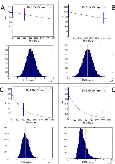
As any dMRI technique, an accurate interpretability of the metrics extracted from the DKI can be challenging and subject to many pitfalls (Jones & Cercignani, 2010). The diffusion and kurtosis estimates can be influenced by noise, motion and image artefacts. In particularly it has been demonstrated that sufficiently large error can cause values that are physically and/or biologically implausible (Tabesh, Jensen, Ardekani, & Helpern, 2011). Therefore to increase the sensitivity and avoid erratic results, it is important to indentify and study the influence of such artefacts and develop more robust methods for data analysis.

1.3. Thesis Objectives and Project Plan

The objective of this thesis is to develop robust methods for pre-processing and analysing DKI data for the Cam-CAN project. Secondly it aims to show the potential of this technique in imaging the brain structural changes across lifespan in the Cam-CAN‟s data recorded so far.

Notably, to improve the robustness of DKI, one can also increase the number of diffusion-weight images (DWIs) required to extract the diffusion and kurtosis tensors. However, since the Cam-CAN project involves the measure of several MRI modalities, the scanning time available for dMRI was limited to 10 minutes. Therefore this thesis is not focus on alternative acquisition schemes. Instead, the quality of DKI metrics will be improved by optimising methods of pre-processing and improving the pipeline analysis of ageing differences across lifespan based on the Cam-CAN‟s pre-selected acquisition scheme of 63 DWIs (acquired on a 3T Siemens Trio with a twice-refocused-spin-echo, 30

(21)

5

diffusion gradient directions for each b-values 1000 and 2000s.mm-2 and three images

acquired using b-value 0, TR=9100ms, TE=104ms, voxel size=2x2x2mm3,

FOV=192x192mm2, 66 axial slices, number of averages=1).

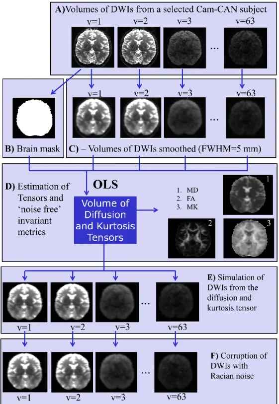
Figure 1.1 shows the project plan on which the work of this thesis is based. The improvement of DKI methods started by studying different fitting methods to extract diffusion and kurtosis tensor from DWIs (October to December of 2011). After studying the behaviour of this different methods on simulated data corrupted by noise, the more optimal methods is selected to estimate the diffusion and kurtosis metrics on real data transformed with different schemes of pre-processing steps (January to February of 2012), which included methods to correct artefacts, as induced by head motion and eddy currents, and methods aiming to remove MRI noise, as steps of downsampling and regularization. The built procedure for DKI is then applied on diffusion MRI data recorded so far by Cam-CAN, and different analysis methods for studying ageing changes on the diffusion and kurtosis data are studied (March to April). At last, the changes observed on the different methods for ageing changes are analysed according to recent brain hypothesis (May to June).

Figure 1.1 – Project plan on which this thesis is based. This figure was presented on the 16th

of January CamCAN’s groups meeting.

(22)

6

1.4. Thesis Outline

After this introduction, the background for this thesis is presented on Chapter 2. This will start with a brief review of the Physics of diffusion (section 2.1). Based on the theory described on the former, section 2.2 will describe how one can use MRI to measure diffusion. The details of diffusion tensor imaging (DTI) is given on section 2.3 which includes its formulation (2.3.1), metrics to extract information from the diffusion tensor (2.3.2), and the noise effects on the accuracy of this technique (2.3.3). The very recent dMRI technique diffusion kurtosis imaging (DKI) is discussed on section 2.4. As for DTI, the details of DKI formulation are given (2.4.1) as well as novel measures that one can use to extract information from the diffusion kurtosis tensor (2.4.2) and its noise influences (2.4.3).

The study of different types of DKI fitting is reported on chapter 3. In this chapter, advances on DKI estimation framework and novel observations of noise artefacts on DKI are described according to the findings of previous studies, as example the published by Tabesh et al (2011) relative to a DKI constrained method that is quickly becoming one of most used methods on recent DKI studies, and the study performed by Jones and Basser (2004) regarding noise influences on DTI.

On chapter 4 the study of reliable pre-processing steps is reported. This will include evidences that algorithms to correct motion artefacts based on registration methods as the ones available in many toolboxes are derisory for dMRI, and result that shows the advantages of using downsampling and regularization algorithms to decrease the impacts of MRI artefacts. In particularly, the optimal value of the size of a Gaussian kernel for noise removal is investigated.

The analysis procedures selected from studying the ageing changes by DKI as well as a description of the preliminary DKI results for the Cam-CAN project are reported in chapter 5. The findings on this chapter will be supported with previous studies, and the impacts of new insights are explored.

On the last chapter (chapter 6), the thesis will be summarized, where the objective accomplished, finding impacts, and future steps are discussed.

(23)

7

Chapter 2

Background

2.1. Physics of Diffusion

2.1.1. Characterization of random translation of particles

Diffusion is a mass process in liquid and gas states which is related to a translation of particles due to thermal energy. This process results in particle mixing without requiring bulk motion as convection and dispersion process (Mori & Barker, 1999). On a molecular level, the thermal energy that each particle carries will result in collisions, and particles will show random translation trajectories known as Brownian motion (Berg, 1993).

In 1905, Albert Einstein introduces the concept of displacement distribution to characterize the Brownian motion of a particle using a probabilistic framework (Einstein, 1956). The displacement distribution quantifies the fraction of particles that travel a specific distance Δr within a particular timeframe t. As example, for a free medium unrestricted by barriers, the probability that one particle have a displacement Δr after a time interval t can be derived from Einstein‟s framework as a Gaussian distribution:

( | ) ( ) _.| |

/, (Eq. 2.1.1)

where D is the diffusion coefficient which depends on intrinsic propriety of the medium as the size and mass of the diffusing particles, the temperature, and the nature of the medium. Media with larger values of diffusion are related to faster dispersion of particles. For example gas states media have larger diffusion coefficient than liquids.

(24)

8

Figure 2.1 – Diffusion process of a two dimensional free medium unrestricted by barriers. Panel A corresponds to an initial state where some central particles were marked in red. After an interval of time t, the marked particles will randomly move in all directions (panel B). The displacement of particles during the instant of time between the positions shown in panel A and panel B can be described with a two dimensional Gaussian distribution of probability, where x and y are the Cartesian components of Δr (panel D). After larger intervals of time the particles will randomly translate over larger areas (panel C) and the Gaussian distribution will have broader shape (panel E). The back circles in panel B and C corresponds to diffusion circles of radius √ .

Figure 2.1 shows the graphical representation of the displacement distribution for particles diffusing in a two dimensional unrestricted medium. These surfaces are concentric once points with the same probability are defined by diffusion circles (Basser, 1995). For example, setting the exponent of Eq. 2.1.1 by the constant ⁄ and assuming that x and y are the components of the two dimensional version of , one can deduce the equation of the diffusion circle with radius√ as:

(25)

9

(√ ) . (Eq. 2.1.2)

Eq. 2.1.2 is of importance since it corresponds to the standard deviation of the displacement distribution. This corresponds to the well-known Einstein formula:

√ . (Eq. 2.1.3)

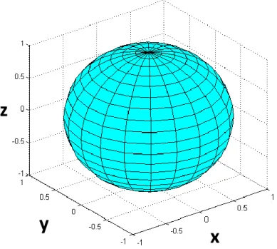
Although Figure 2.1 described diffusion on a two dimensional space, similar observations and derivations can be performed easily for three dimensional cases by assuming three Cartesian components x, y, and z for the displacement vector . In this case Eq. 2.1.1 will be described by a three dimensional Gaussian distribution, and the points with the sane probability will define surfaces with spherical geometries – the diffusion spheres (Basser, 1995). For example, defining the constant ⁄ on the exponent of Eq.2.1.1, the equation of a 3 dimensional diffusion sphere surfaces with radius √ can be written as:

(√ ) (Eq. 2.1.4)

The diffusion sphere described by Eq. 2.1.4 is graphically represented on Figure 2.2.

Figure 2.2 – Diffusion sphere showing the surface of a mean square three dimensional displacement for an isotropic medium.

(26)

10

2.1.2. Classical diffusions laws and relation with diffusion atomic view

Although, it was only in 1905 that diffusion was described from an atomic perspective, the concept of the diffusion coefficient have already been introduced earlier by Fick (Fick, 1855). Based on extensive investigations on the diffusion of salts in water, Fick stated that under a gradient of concentration 𝛁C and assuming a medium with diffusion coefficient D, the flux of diffusing particle J can be described as:

𝛁 (Eq. 2.1.5)

From Eq. 2.1.5 one can deduce a null flux of particles for a null gradient of concentration. However, such situation does not mean that particles are not in influence of diffusion process. According to the law of large numbers of the probability theory (Jaynes, 2003), the number of particles crossing a section of area in one direction will be the same from the opposite (null net flux) once the number of particle are uniformly distributed. In the other hand, if a gradient of concentration is present, one side of the medium delimited by a section of area will have a larger number of particles, and therefore it will be more likely that a larger number of particles from that higher concentrated region will cross the section of area. For instance, in the case described on Figure 2.1, since initially the particles are high concentrated on the centre of the medium, they are more likely to spread in a radial symmetry, and the net flux will be positive in direction from the centre to the periphery. The migration of the particles will results in a decrease of the concentration gradient, reaching a steady state where the concentration is uniform across the medium. By combining Eq. 2.1.5 with the conservation of mass equation:

( ) ( ) (Eq. 2.1.6)

one can obtain the expression that describes the variation of concentration of a medium, i.e. the Fick‟s second law (Wilkinson, 2000):

(27)

11

As mentioned in section 2.1.1, from Einstein‟s framework the distribution of particle displacement in a free diffusion medium is derived as a Gaussian distribution. Such result is also supported by the second Fick‟s Law (Jaynes, 1989). As the probability

P of finding a particle per unit of volume is proportional to the concentration, Eq. 2.1.7

can be rewriting in function of P:

𝛁 ( ) ( ) (Eq. 2.1.8)

Knowing the initial position r0 of a particle, one can write the function of the distribution of probability in the time instant t=0 as an impulse function δ:

( | ) ( ) (Eq. 2.1.9)

Using this initial condition, one can resolve Eq. 2.1.8 as the Gaussian distribution for a free medium unrestricted by barriers:

( | ) ( ) _.| |

/ (Eq. 2.1.10)

where is the particle displacement .

2.1.3. Diffusion tensor for characterizing anisotropic media

In the previous sections diffusion is characterized by a single scalar coefficient. This approach is sufficient for media where diffusion does not depend in spatial direction, i.e. isotropic diffusion. However this situation is not always valid – for some media, particles can have more difficulty on translating over some specific directions. This is the case of media formed by oriented structures or microstructures that makes diffusion anisotropic (Basser, Mattiello, & LeBihan, 1994a).

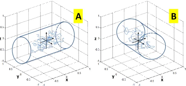
An example of anisotropic media is shown in Figure 2.3.A in which particles are confined to a cylindrical shape tube. In that case, particles are free to randomly translate in x direction while along the y and z directions they are limited by the walls of the tube, and thus diffusion is higher along the x direction than those along y and z.

(28)

12

Figure 2.3 – Representation of two media restricted by cylindrical tubes. In Panel A particles are free to translate along direction x, while along x and z they are limited by the boundaries of the tube. In opposite to panel A, panel B is not oriented with the frame of reference x-y-z, and thus particles are free to translate only on an oblique direction.

Defining , and as the diffusion coefficient along the axis x, y and z, the first Fick Law for the case described in Figure 2.3.A can be written as:

* + * + *

⁄ ⁄ ⁄

+. (Eq. 2.1.11)

For more general cases where the cylindrical geometry is not aligned with the frame of reference defined by the axis x, y and z (Figure 2.3.B), Fick‟s Law is only full described with a 3x3 diffusion tensor (Basser, 1995; Basser et al., 1994a):

* + * + * ⁄ ⁄ ⁄ +. (Eq. 2.1.12)

In a similar way to what was described in the previous section for the isotropic media case, the displacement of distribution of the cylindrical anisotropic media can be derived from Eq. 2.1.12 as:

( | )

√( ) ( ) .

( ) ₍ ₎

(29)

13

where is the diffusion tensor:

*

+ . (Eq. 2.1.14)

Similarly to the scalar diffusion coefficient D for isotropic media which have to be defined by a positive number for being physically plausible, the diffusion tensor D have to be defined by a positive matrix (Koay, Carew, Alexander, Basser, & Meyerand, 2006), i.e: (1) D have to be symmetric ( = ), (2) all the diagonal elements of D have to be

positive, and (3) all the determinants of all the leading submatrix have to be positive. Due to the symmetric propriety, D can be rewritten only with six independent elements ( ): * + . (Eq. 2.1.15)

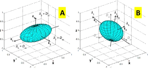
As the isotropic diffusion can be geometrically represented on a 3D space with a sphere, the anisotropic diffusion tensor can be represented geometrically by a 3D ellipsoid (Basser, 1995), where the six independent elements of D fully described its size, shape and orientation (see panel A and B of Figure 2.4 which represents the diffusion ellipsoid for the cases described on Figure 2.3). For example by defining the exponent of the displacement distribution on Eq. 2.1.13 to a constant we can obtain the expression (Basser, 1995):

( ) ( )

( ) ( ) ( ) (Eq. 2.1.16)

(30)

14

, - [

] 6 7 (Eq. 2.1.17)

The length and direction of the three orthogonal principal axes of the diffusion ellipsoids (see Figure 2.4) can be decoupled by the following matrix decomposition of D (Basser, Mattiello, & LeBihan, 1994b):

* + [ ] [ ] [ ] (Eq. 2.1.18)

where λ1, λ2 and λ3 are the three eigenvalues related to the values of diffusion along the

three principal axes of the diffusion ellipsoid, while the triplets of number ( ), ( ), and ( ) are the eigenvectors which gives the direction of each principal axis. In particularly, vector( ) and λ1 corresponds to the values of the

ellipsoid axis with larger length.

Figure 2.4 – Geometrical representation of the diffusion tensor for the two isotropic media represented in Figure 2.3. Since diffusion ellipsoid in panel A is aligned with the frame of reference x-y-z, the eigenvalues λ1, λ2, and λ3 corresponds to the tensor elements Dxx, Dyy, and

Dzz. On the other hand, for panel B, the eigenvalues can be computed by matrix decomposition

shown by Eq. 2.1.18.

(31)

15

2.2. MRI and Diffusion

In MRI, subjects are exposed to a strong magnetic field and the magnetic moments of the water protons (also referred as spins) start to precess (i.e. rotate) around the direction of magnetic field (Conolly et al., 2000). The magnetic moments can then be described by two components: a longitudinal component aligned to the magnetic field and a transversal component perpendicular to the magnetic field. If within a voxel the spins are precessing in phase, the net transversal component can be measured by the MRI receive coils. To increase the transversal component and have a significant signal to measure, it is applied specific radio frequency (RF) pulses to insure that spins within a voxel are in phase (McRobbie, Moore, Graves, & Prince, 2003). As example, in the commonly used spin eco sequences (Figure 2.5), two RF pulse are applied: 1) a pulse of 90º is applied simultaneously with a gradient to selectivity stimulated the spins of a slice of the body; 2) after the phase and frequency gradient which encodes each voxel with a specific frequency and phase, a 180º pulse is applied to realign the spins within a voxel and reproduce a measurable signal referred as the echo (McRobbie et al., 2003).

Figure 2.5 – Spin eco sequence

(32)

16

2.2.1. Pulsed gradient spin echo (PGSE)

MRI can be used to quantify the diffusion of the brain using proper sequences (Basser et al., 1994a). One basic and commonly diffusion sensitizing gradient is an adaption of the spin eco sequence called pulsed gradient spin echo (PGSE). Relative to the spin eco sequence, PGSE have two extra gradients, one after the 90º RF pulse and other after the 180º, Figure 2.6. The objective of the first additional diffusion gradient is to add a phase shift ( ) that will depend on the spin position r relative to the direction of the additional gradient field (Johansen-Berg & Behrens, 2009) as described by the following equation:

( ) ∫ , (Eq. 2.2.1)

where is the gyromagnetic ration which depends on the type of the atomic nuclei (for protons is 42.56 MHz T-1), the intensity of the diffusion gradient and its duration. The second diffusion gradient is applied after a time interval inducing an opposite phase shift. Such shift has the same amplitude than the previous one since both gradient pulses have the same values of intensity and duration ; however it has an opposite effect once applied after the 180º RF pulse which inverted the protons phase for spin realignment. Therefore, and assuming that the duration of each diffusion pulse is much smaller than the time interval , the total shift induced on a spin can be expressed as:

( ) , (Eq. 2.2.2)

where is the displacement of the proton spin relative to the direction of the diffusion gradient on the time interval .

Eq. 2.2.2 suggest that voxels related to protons that have larger displacements will present spins precessing in a ampler range of phase, while voxels that are less conditioned by the diffusion process will have proton with negligible phase shift. MRI receive coils will therefore measure smaller intensities for voxels related to media with larger diffusion coefficients (spins that are precessing out of phase) and larger intensities for voxels related to media with smaller diffusions coefficients (spins possessing in phase).

(33)

17

Figure 2.6 – Representation of the two additional diffusion gradients on the pulsed gradient spin eco. This figure was adapted from (Correia, 2009).

The phase shift ( ) described in Eq. 2.2.2 can mathematically be expressed in order to the diffusion coefficient D. Given that the total magnetization within a voxel is a sum over all individual magnetic moments :

∑ { ( ) }, (Eq. 2.2.3)

and the spin population can be described with a displacement distribution of ( | ), the amplitude of the signal attenuation can be calculated as:

∫ { ( ) } ( | ) , (Eq. 2.2.4)

where is the signal that should be detected if no diffusion gradient is applied. Assuming the Gaussian displacement distribution described by Eq. 2.1.1, Eq. 2.2.4 can be rewrite as:

(34)

18

It is notable that for Eq. 2.2.5 one can verify that voxels with larger diffusion coefficient are related to lower intensities measured by the MRI receiver coils. Moreover, one can see that larger signal attenuation can also be related to larger water particles displacements if diffusion-weighted signal is measured using larger diffusion time values. Gradients with larger amplitude and duration will also highlight the diffusion contrast, once they induce larger phase shift on diffusing water molecules.

2.2.2. The Stejskal-Tunner equation

The more general relationship between the diffusion coefficient and the signal measured in diffusion MRI was established in 1965 by Stejskal and Tunner. Defining the applied diffusion gradient field ( ) as:

( ) . ( ) ( ) ( )/ (Eq. 2.2.6)

and describing an arbitrary function ( ) as:

( ) ∫ ( ) (Eq. 2.2.7)

the MRI measured diffusion-weighted signal S can be expressed with the Stejskal-Tunner equation as:

, ⁄ - ∫ ( ( ) . / . /)

( ( ) . / . /) , (Eq. 2.2.8)

where is the MRI measured signal when the diffusion gradient is not applied, ( ) the Heaviside function, TE the time interval between the instant that MRI sequence was applied (t=0) to the instant when the echo is recorded (see Figure 2.5), and D the scalar diffusion coefficient. By defining the parameters that are only dependent on the diffusion gradient by a single constant b (known also as b-value):

(35)

19

∫ 4 ( ) ( ) ( )5

( ( ) . / . /) , (Eq. 2.2.9)

the notation of Eq .2.2.5 can be simplified as:

* +. (Eq. 2.2.10)

Remarkably, Eq. 2.2.10 is of importance because it shows how easily one can estimate a diffusion coefficient. D can be computed on each voxel by linearization of Eq. 2.2.10:

. /. (Eq. 2.2.11)

where values of S can be acquired with a diffusion-weighted image (DWI) while values of acquired by setting the diffusion gradient to zero (i.e. b-value equal zero). Moreover, the b-value can easily be computed off-line with the known parameters of the diffusion gradient sequence using Eq. 2.2.9 (Mattiello, Basser, & LeBihan, 1994). For example, assuming the PGSE on Figure 2.6, the expression for the b-value can be derived from Eq. 2.2.9 as:

. /. (Eq. 2.2.12)

For a PGSE acquisition where gradient duration is much smaller that the time interval , Eq. 2.2.12 can be even simplified as:

. (Eq. 2.2.13)

Notably, Eq. 2.2.13 corresponds to the case described in section 2.2.1, and therefore if we apply this equation to Eq. 2.2.10, Eq. 2.2.5 is rewritten.

(36)

20

2.2.3. Twice Refocused Spin Echo (TRSE)

Since an MRI acquisition requires time-varying gradients, non-desired electric currents (named as eddy currents) are induced on the nearby conductors. This will generate local magnetic field gradients that will be either added or subtracted from the phase and frequency encoding gradients, and therefore MRI images will show spatial distortions (Jones & Cercignani, 2010). This artefact is not problematic in most of MRI modalities since the rising and falling of the encoding gradients are normally close in time which induces a cancellation of eddy currents. However, due to limitations of the gradient amplitude G on the current clinical scanners, dMRI requires diffusion gradients with larger duration to achieve b-values that provides robust estimations of diffusion coefficient (normally around 1000 s.mm-2). Therefore for dMRI the rising and falling of the diffusion gradient are not close in time and eddy current distortions are significant.

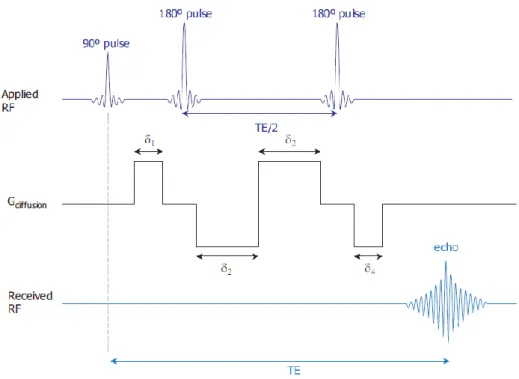
The Twice Refocused Spin echo (TRSE) sequence was developed with the aim of reducing eddy distortions at no cost in scanning efficiency or effectiveness (Reese, Heid, Weisskoff, & Wedeen, 2003). TRSE uses two 180º pulses (refocusing pulses) and the effects of the eddy currents are cancelled with two bipolar diffusion gradients of length

and , Figure 2.7

Figure 2.7 – Representation of the twice refocused spin echo sequence. This figure was adapted from (Correia, 2009).

(37)

21

2.3. Diffusion Tensor Imaging

In neural tissues, the water molecules and metabolites are under the influence of diffusion processes. They are constantly bouncing, crossing and interacting with many tissue components as cell membranes, cytoskeleton and macromolecules (Johansen-Berg & Behrens, 2009). Diffusion process depends on microstructure, being sensitive to the number, orientation, and permeability of barriers as myelin, and to the presence of various cell types of organelles as dendrites, axons, neurofilaments and microtubes (Denis Le Bihan et al., 2001). Furthermore, since the microstructures are highly oriented, diffusion depends on spatial direction (M. E. Moseley et al., 1990). For example, in brain white matter the water molecules will have higher mobility in the direction of the fibres tracks than across the myelinated barriers of the neural axons, i.e. diffusion in the direction of the fibres is larger than in perpendicular directions (Basser, 1995). In opposite, diffusion will show isotropic proprieties in grey matter once this type of tissue does not consist on oriented structures.

As mentioned in section 2.1.3, anisotropy in media with cylindrical geometry can be fully described using a diffusion tensor. Assuming that neural tissue consist of white matter tracts which can be modelled as cylindrical tubes, such approach can be useful in modelling the dependence of diffusion on biological tissues (Mori & Barker, 1999).

Proposed by Basser et al. 1994, diffusion tensor imaging (DTI) uses the information of diffusion-weighted images (DWIs), obtained with different diffusion gradients, to provide a non-invasive estimation of the diffusion tensor for all the voxels of a brain volume (Basser et al., 1994a). Over almost two decades since it was development, DTI had become an established technique which had shown to provide subtle information of neural structures for several clinical studies as cerebral ischemia, brain maturation, traumatic brain injury, epilepsy, multiple sclerosis and Alzheimer‟s disease (for a review of several clinical applications of DTI see Sundgren et al., 2004). Moreover, DTI can provide information for algorithms of fibre tracking which can be an important technique in studying brain connectivity (Fillard et al., 2011).

2.3.1. The formulation beyond DTI

DTI was based on the adaption of the Stejskal-Tanner equation for anisotropic mediums (Stejskal, 1965):

(38)

22

, ⁄ - ∫ 4 ( ) ( ) ( )5

( ( ) . / . /) , (Eq. 2.3.1)

where and are the MRI measured signal with and without applying an diffusion gradient, ( ) the Heaviside function, ( ) the function defined by Eq. 2.2.7, TE the time interval between the instant that MRI sequence is applied (t=0) to the instant that the echo is recorded, and D the diffusion tensor. By analogy with the scalar b-value in section 2.2.2, it is possible to define a matrix which only depends on the parameters of the diffusion gradient (Basser et al., 1994a):

∫ 4 ( ) ( ) ( )5

( ( ) . / . /) , (Eq. 2.3.2)

therefore, Eq 2.3.1 can be rewritten as:

* +, (Eq. 2.3.3)

where „:‟ is the generalized dot product. Matrix B is a symmetric 3x3 matrix:

*

+ . (Eq. 2.3.4)

As the scalar b-value, B can be computed off-line (Mattiello et al., 1994). For example, for a PGSE gradient ( ) [ ( ) ( ) ( )] with duration and a time interval between diffusion pulses , the elements of the B matrix can expressed as:

(39)

23

Alternatively, the matrix B can also be computed from the scalar b-value and then combined with an 3x3 matrix containing the gradient direction information, as shown in the following equation:

[ ] (Eq. 2.3.6)

where ( ) is the unit vector that describes the direction of the diffusion gradient G.

Since D and B are symmetric matrixes, Eq. 2.3.3 can be simplified and expanded in function of individual and elements as:

*

+, (Eq. 2.3.7)

or in order of the scalar b-value and the gradient direction as:

( ) , ∑ ∑ - = * }, (Eq. 2.3.8)

where index 1, 2, and 3 correspond to the spatial dimensions x, y and z.

The six independent elements of the diffusion tensor can be extracted from at least

N=7 DWIs. This 7 images have to be recorded for at least six non-collinear diffusion

gradients directions and at least 2 different b-values which can include b=0 s.mm-2. The estimation of diffusion parameters from DWIs can be achieved by different methods (Koay et al., 2006) which varies from linear least squares approaches to non-linear ones. Moreover depending on the robustness of each method, one can add constrains which can force the diffusion metrics to physically and biologically plausible ranges or weights to correct non-uniformity of diffusion-weighted signal variance. Examples of some of these approaches are described below.

(40)

24

Linear least squares

Eq. 2.3.3 can be converted to a linear framework by taking the logarithm on each side of the equation (Basser et al., 1994b). For example, from the expansion described on Eq. 2.3.8 we can write:

( )

. (Eq. 2.3.9)

By defining a column vector with all the logarithms of the N measures of ( ), writing the matrix with the information of the b-values and gradients directions used in each measurements as:

* ( ) ( ) ( ) ( ) ( ) ( ) ( ) ( ) ( ) ( ) ( ) ( ) ( ) ( ) ( ) ( ) ( ) ( ) ( ) ( ) ( ) ( ) ( ) ( ) ( ) ( ) ( ) ( ) ( ) ( ) ( ) ( ) ( ) ( ) ( ) ( ) + (Eq. 2.3.10)

and defining the vector which elements are the diffusion tensor elements and the logarithm of :

, - , (Eq. 2.3.11)

Eq. 2.3.9 can be rewritten as:

. (Eq. 2.3.12)

From Eq. 2.3.12 the unknown parameters on can be estimated from the standard linear least squares solution:

(41)

25

where ̂ is the estimation of vector and the pseudoinverse of matrix . This approach was followed on several studies due to its implementation simplicity and for providing algorithms with high computation speed efficiency (Jones & Cercignani, 2010).

Weighted Linear least squares

The linear least squares solution described by Eq. 2.3.13 assumes that the elements of vector have errors with independent and identically distributed variance. In fact, when signal to noise ratio is sufficiently high, measures of the diffusion-weighted signal can be assumed to have a uniform variance. However, it is important to note that using a linear framework we are not using the diffusion-weighted signals but their log-transformed versions. For standard error propagation techniques (Jones & Cercignani, 2010) one can deduce that assuming diffusion-weighted signals with uniform variance of , the variance of the log-transformed version can be described by:

, (Eq. 2.3.14)

where is the noise free version of S. Approximating the exact value of by the measured value ( ) and measuring from noise power estimation algorithms, (e.g. Aja-Fernandez, Alberola-Lopez, & Westin, 2008), one can compute an covariance matrix where diagonal elements are the values of . The information of matrix can be incorporated on the estimation of using the more general linear least squares solution (Jones & Cercignani, 2010) given by the following equation:

̂ 0 1 . (Eq. 2.3.15)

This approach should provide a more accurate estimation once each log-transformed diffusion-weighted signal is weighted by its variance.

Non-Linear least squares

For the non-linear least squares solution, the tensor is estimated directly from Eq. 2.3.3 using well established methods as the Levenberg-Marquardt non-linear regression (Jones & Basser, 2004). Such non-linear approaches involve iterative algorithms where the

(42)

26

elements of diffusion tensor are adjusted till the errors between the predicted signals and the measured ones are minimized. The objective function to be minimized can be described as: ( ) ∑ ( ( ) ∑ ) (Eq. 2.3.16)

Since this non-linear fit deals directly with the diffusion-weighed signals, the variance of the measured insets should be uniform (if signal to noise ratio is sufficiently high) even without applying any kind of approximation as assumed by the weighted linear solution described in Eq. 2.3.15. Therefore, it is expected that non-linear least squares approaches will have a better accuracy than the ones mentioned above. Nevertheless, iterative algorithm can be disadvantageous for being very computationally demanding. A strategy to reduce such disadvantage is to initialize the iterative process with results obtained from Eq. 2.3.13 or 2.3.15. This also have the advantages of avoiding convergence to a global minimum (Jones & Cercignani, 2010).

Constrained linear and non-linear least squares

Constrains can be applied in the minimization approach to avoid that data influenced by noise motion and artefacts result on physical or biological implausible values of diffusion (Koay et al., 2006). This can be applied on the non-linear approach described above (Eq. 2.3.16) or on the linear framework by minimization the following function:

( ) ∑ ( ( ) ∑

)

(Eq. 2.3.17)

However, when applying constrains both linear and non-linear techniques will be computationally demanding once they both require iterative approaches or non-linear formulations. For example, constrains can be incorporated on each step of an iterative algorithm so that is forced to converges to a solution according to imposed restrictions. Alternatively the diffusion tensor can be directly constrained on the DTI formulation matrix using for example the Cholesky parameterization (Koay et al., 2006). Assuming

(43)

27

that all and only positive matrices can be decomposed into the product of a lower triangular matrix, the positive diffusion tensor can be decomposed as:

[ ] [ ] [ ] * + . (Eq. 2.3.18)

Consequently the optimization problem on Eq. 2.3.16 or Eq. 2.3.17 can be rewritten in a way that elements are iteratively estimated, instead of the elements . Diffusion tensor will then be estimated using Eq. 2.3.18 and since computed by the product of a lower triangular matrix it will mandatory be defined with a positive matrix, reflecting physically plausible values.

2.3.2. DTI invariant Measures

From the estimated diffusion tensor, several rotationally invariant scalar measures can be calculated. These parameters can be as important as identifying fibre direction (Pierpaoli & Basser, 1996). Examples of invariant parameters are the mean diffusivity (MD), the fractional anisotropy (FA), axial diffusivity ( _∥), and radial diffusivity ( ).

Mean diffusivity can be calculated as Eq. 2.3.19 and gives an overall of the mean-squared displacement of molecules i.e. average of diffusion ellipsoid size (Denis Le Bihan et al., 2001):

( ) _{〈 〉}

(Eq. 2.3.19)

where „Tr‟ is the matrix trace.

The axial diffusivity gives the magnitude of the diffusion along the principal ellipsoid component, so it is equal to λ1:

∥ (Eq. 2.3.20)

For example in white matter, since the first principal axis of the diffusion ellipsoid is align with the fibre direction, ∥ is of interest because corresponds to the diffusion value

(44)

28

along the direction of fibres, and thus it is believed to be an index of axonal integrity (Helpern et al., 2011).

In the other hand radial diffusivity is the mean diffusion along the orthogonal components relative to the principal ellipsoid axis, which can be estimated as the average between λ2 and λ3:

(Eq. 2.3.21)

In opposite to the axial diffusivity, in white matter is related to the average of the diffusion values in the directions across the fibre barriers which consists on structures as the axonal myelin, and thus it is believed to be an index of myelin integrity (Helpern et al., 2011).

Fractional anisotropy (Pierpaoli & Basser, 1996) measures the anisotropy in a range between 0 (case of isotropic diffusion, λ1= λ2= λ3) to 1(fully anisotropic λ1>> λ2= λ3=0):

√ ,( 〈 〉) ( 〈 〉) ( 〈 〉)

-√ ( )

, (Eq. 2.3.22)

therefore structures that give diffusion high anisotropy proprieties, as single oriented populations of white matter fibres, are related to FA values close to one, while brain regions which are not oriented on specific direction, as grey matter regions, are related to low or even null values of FA.

2.3.3. Effects of noise on DTI

MRI as any other imaging technique is influenced by noise (Sijbers, den Dekker, Scheunders, & Van Dyck, 1998). The complex valued data acquired by MRI coils are corrupted by noise that is typically well described by a Gaussian distribution on both real and imaginary space. When the complex data in K-space is converted to an image in spatial domain using Fourier reconstruction, the Gaussian noise in real space and imaginary space is converted to Rician noise which corrupted intensity of each voxel image is given by:

√.