EDP - A new estimation algorithm

(1)

1

A Work Project, presented as part of the requirements for the Award of a Masters Degree in Management from the NOVA – School of Business and Economics.

EDP – A New estimation algorithm

Frederico Medeiros 748

A Project carried out on the Operations Management course, under the supervision of: Prof. Dr. Luís Catela Nunes

(2)

2

Abstract

The aim of this work project is to analyze the current algorithm used by EDP to estimate their clients’ electrical energy consumptions, create a new algorithm and compare the advantages and disadvantages of both. This new algorithm is different from the current one as it incorporates some effects from temperature variations. The results of the comparison show that this new algorithm with temperature variables performed better than the same algorithm without temperature variables, although there is still potential for further improvements of the current algorithm, if the prediction model is estimated using a sample of daily data, which is the case of the current EDP algorithm.

(3)

3

1. Introduction

The main objective of this work project is to create a new algorithm, able to make more precise electricity consumption estimations for EDP’s clients.

But why do electricity companies need a good estimation method for their client’s electricity consumption? There are many answers to this question. First of all, it is important to know that, on average, EDP is able to obtain their customers’ consumption readings only every three months. On the other hand, EDP’s clients are billed either every month or every two months, creating the necessity of having a good prediction of the amount of electricity consumed every month.

Not having a good estimation may have negative consequences not only for their clients, but also for the company itself. On the one hand, if the predicted consumption is far from the real consumption, this would imply that a client would be either overcharged or undercharged. Both cases would have a nefarious effect on the clients’ opinion about the company, as these cases usually imply big billing readjustments. On the other hand, a good algorithm also impacts the company in other ways; for instance, proper estimations are necessary to obtain a good financial plan. The same would apply to the operations department. Another reason for the need of this new algorithm is that it allows a better estimation of the energy losses between power plants and final consumers. This is very important for the company, as it gives the company information about the efficiency of their distribution networks, for example.

Another advantage present in a more refined algorithm is its usage in tests/experiments that require good estimations. A good example is the current experiment being

(4)

4

conducted by EDP in Évora, where the company is testing the impact of new products and services based on “smart meters” which are able to report the clients’ readings everyday. These devices are already implemented in the city of Évora but it will still take about 10 years to be fully implemented in the whole country. Besides these studies, a new algorithm may as well be used by other electricity companies, either Portuguese or from other countries.

In order to perform this work project, it was necessary to observe and understand the current algorithm, so as to discover some of its flaws as these were actually a good starting point. Additionally, it was taken into account that this algorithm would be used to estimate thousands of consumptions every day, so although a better and more precise algorithm could be created, this one needed to be simple enough in order to run smoothly through the company’s system and databases.

In order to test the performances of the current and the new algorithms, a database of EDP’s clients was used. This database is considered by EDP as a representative sample of the company’s customers. This database has around fifty thousand readings from EDP clients with different consumption patterns. To obtain the new algorithm and test the algorithms, the database was divided in 3 groups: Profile A – Clients with a contracted power of over 13,8 kVA; Profile B – Clients with a contracted power up to 13,8 kVA and an annual consumption of over 7140 kWh; Profile C – Clients with a contracted power up to 13,8kVA and an annual consumption up to 7140kWh.

(5)

5

The current EDP algorithm is based on a fixed yearly seasonality pattern of electricity consumption, estimated using daily historical data. As such, this algorithm is not able to take into account the temperature fluctuation registered during the year. To create the new algorithm, some variables related to temperature were added. As the results in Bessec and Fouquau (2008) suggest, when the temperature of a country is over a certain threshold, there is an extra consumption of electricity, in order to obtain a cooling effect. On the other hand, when the temperature drops below another threshold, there might be an extra consumption of electricity, in order to obtain a heating effect. Both effects were implemented in the new algorithm.

In the next section, the methodology used to obtain the new algorithm and to test the algorithms will be explained, followed by the results obtained from the previous tests. In the final section of this work, we may see the main findings, as well as the problems faced in this study and the recommendations for future works.

2. Methodology

The idea in this work was to be able to estimate consumptions for different periods of time, either from periods of 2 or 3 months, that could be required for billing purposes, as for periods of 1 year, which would be very useful for a financial analysis, for example.

(6)

6

It is also important to state that the data available for each client is the exact consumption of that client, in given periods of time. These periods of time have an average length of 3 months.

For a better understanding of the current algorithm and the new one, the methods used to obtain them and the criteria used to test them are described below.

2.1. Current algorithm

In order to better understand the current algorithm, in this section is presented a brief explanation of how it works and its weaknesses:

( ) ∑

Where

Where, t1 stands for start of period, t2 for end of period, CBR for consumption between

readings

The current algorithm is composed by three elements, a profile, a daily average consumption and the number of days.

The profile

The seasonality profile (Pt) is incorporated in this formula, so that it can add an effect of

(7)

7

In order to calculate it, this algorithm calculates an average of the profiles correspondent to each of the days that need to be estimated.

EDP obtains these profiles, using the “Diagrama de Carga de Referência” and “Diagrama de Carga do Sistema”, published annually by ERSE – Entidade Reguladora dos Serviços Energéticos. Another relevant fact is that these profiles were created using data obtained from clients who had a special device installed, built to record consumption for every 15 minutes period, during the year of 2004.

The daily average consumption

The daily average consumption (DAC) is incorporated in this algorithm as it adds an historic consumption to this algorithm.

EDP calculates this daily average consumption using the previous readings, calculating an average consumption starting twelve months before the last reading and ending in the last reading.

Number of days

The number of days (Nd) is incorporated in the algorithm, referring to the number of days of the period that we need to estimate.

Weaknesses

Analyzing this algorithm, we may see that it has two main weaknesses. First of all when calculating the daily average consumption, sometimes it might be necessary to use data from a reading made 24 months ago, for example, that might be outdated as

(8)

8

consumption habits may change a lot in two years. On the other hand, this algorithm also uses outdated data when obtaining the profiles as the data used to create them for a certain year is always data from the previous year.

2.2. The new algorithm

In order to better understand the new algorithm, below is a brief explanation of how it works, how it was obtained and its strengths and weaknesses:

2) ( ) ∑ Where, ( ) Where, { {

Where, t1 stands for start of period, t2 for end of period, RDAC for real daily average

(9)

9

The new algorithm is composed by three elements, a profile, a historic daily average consumption and the number of days.

The profile

The profile (Pt) is incorporated in this formula, so that it can add an effect of

seasonality, since consumption fluctuates throughout the different periods of a year.

To create these profiles, the real daily consumptions from the whole sample in the years of 2006, 2007 and 2008 of the database were used, in order to create a daily average of the total consumption of the sample. The next step was to normalize these averages. To do that, the daily averages were divided by the average of the average daily consumptions. The following step was then to statistically estimate the relationship between temperature registered in a day and the electricity consumption of that day. So that it could be accomplished, a linear regression analysis was performed. To start with, all the months of the year except January, were taken as dummy variables, and two other variables were added: one to represent the effect of extra electricity spent to cool the temperature if it is above a certain threshold; and another variable to represent the effect of extra electricity spent to heat the temperature when the temperature is below another threshold. In order to find the best values for the heating and cooling limits, many values were tested, where the values chosen for these thresholds were the ones that presented the higher Rsquare and therefore the ones that best fit the data. With the results of the regression, the relationship between temperature registered in a day and the electricity consumed that day was then proven. The cooling effect was found significant for profile C, while the heating effect was found significant for all the profiles.

(10)

10 The historic daily average consumption

The historical daily average consumption (HDAC) is incorporated in this algorithm as it adds an historic consumption to this algorithm. The idea here was to be able to have an average historical consumption, in order to have a good starting point for the estimations.

In order to calculate this, an exponential moving average is used. With this method, it was possible to attribute a weight to all the readings before the last one and another weight to the last reading. It differs from the current average used by EDP as the current method uses an average that takes into account mostly information from the last year consumption, while this method takes into account the life time consumptions and the consumption in the previous period. As we can see in equation 2, the weight of 0.6 was attributed to the readings before the last one and the weight of 0.4 was attributed to the last reading. These weights were obtained, minimizing the squared error between the estimations of the electricity consumption and the real electricity consumption.

Number of days

The number of days (Nd) is incorporated in the algorithm, referring to the number of days of the period that we need to estimate.

Weaknesses and strengths

Since this algorithm uses an exponential moving average in order to calculate the historic average, the fewer the previous readings available for each client, the higher the chance of having outdated data being used. On the other hand, the fact that this

(11)

11

algorithm uses information from the daily temperature registered on each of the days that we need to estimate, introduced at least a daily factor which is easily obtainable in this formula, where the current algorithm only uses past data. Another positive aspect of this new algorithm is that its daily average consumption does not rely only in data from one or two years, as these years might have had and abnormally low consumption or an extraordinary high consumption.

2.3. Algorithm without temperature effects

So that we could do a better evaluation of the new algorithm, a parallel algorithm which does not include temperature effects was made. Created exactly the same way, this algorithm only differs from the previous by not having a heating or a cooling variable.

2.4. Evaluation Criteria

In order to test the three algorithms, estimations were made for the periods of the database in the years of 2006, 2007 and 2008. Then some more estimates were made for the year of 2009. It was very useful to test the models for 2009, since we were able to obtain results for a year which was not contained in the data used to obtain the seasonal profiles, and therefore it should be an unbiased year

So that the new and the current algorithms can be compared and evaluated, some evaluation criteria were necessary. Many criteria were used since there are many interesting ways to analyze their performance.

(12)

12

One of them was the mean absolute error. Using it made it possible to understand how precise the algorithms were. It allowed us to perceive how high was the average error, regardless of the negativity or positivity of this error. In order to calculate it we needed to subtract the estimated consumption from its correspondent real daily consumption and then calculated the average of those absolute values.

∑ ( )

Another criterion used was the mean squared error. Using it and comparing it with the absolute error average made possible a conclusion about the variability of these errors, as it gives a higher weight to higher errors and a lower weight to lower errors. In order to calculate it we needed to subtract each estimated consumption from its correspondent real daily consumption and square the result. Then the average of those values was calculated.

∑

The following criterion used was the mean error. Using it made it possible to discern if there is an overestimation or underestimation the value of electricity consumption. A value below 0 would mean that the clients were over charged, while a value above 0 would mean that clients were undercharged. In order to calculate it, the estimated consumption was subtracted from the correspondent real daily consumption and then, the average of those values was calculated

The last criterion used was the 5th and the 95th percentile. It was used to check and compare extremity values of the estimates, as this criterion allows us to check how far

(13)

13

away from 0 (as a value of 0 would mean that there is no error) is the error correspondent to the 5th percentile and how far away from 0 is the 95th percentile. In order to obtain them, the percentile function of Microsoft Excel was used, using as target data the error values.

3. Results

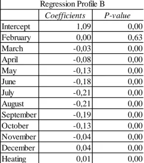
So that a relationship between electricity consumption and temperature could be proven a regression for each of the three profiles, A, B and C, was done. The first regressions made for the profiles A and B presented their cooling variable as a non-significant as their respective p-value was above 0,05. Therefore they had to be re-estimated, excluding this variable. On table 1, we may see that on the new regression estimated for profile A, it can be assumed that a relationship between an increase in electricity consumption and the registered temperature exists , since the presented p-value is way lower than 0,05. That same relationship may be assumed on the regression for the profile B since, as we can see on table 2, the p-value correspondent to that variable is also lower than 0,05.

If we take a look at table 3, we may see that not only the heating variable presents a significant value but the cooling variable as well, since both present a quite low p-value, under 0,05.

(14)

14

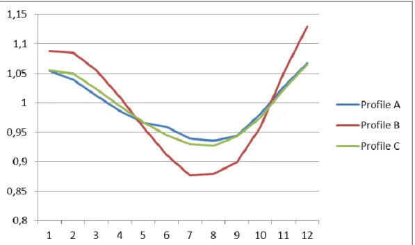
In Figure 1, we may see the monthly seasonality effect of electricity consumption on Profiles A, B and C. A higher consumption is noticeable during colder months, while consumption decreases during the other periods.

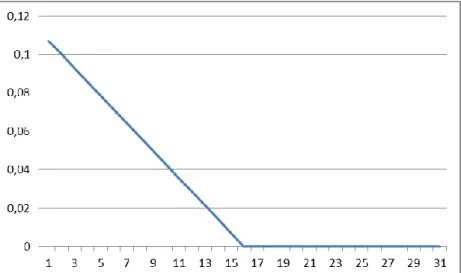
In Figures 2, 3 and 4, the effect of heating on the profiles A, B and C, respectively may be seen, as well as the effect of cooling, verified only on profile C. we can see that on average, when the temperature drops below 15ºC, the lower the temperature, the higher the consumption of energy. On the other hand it is noticeable on the profile C that when the temperature rises above 23ºC, the higher the temperature, the higher the electricity consumption used with a cooling purpose.

Profile A

With the estimations made, in order to analyze and compare the algorithms, some criteria were used.

In table 4, it is shown that the lowest value of the 95th error percentile for the first years was the one from the new algorithm without heating, with a value of 16.24 which means that the top 5% of the errors from the new algorithm without heating are higher than 16,24. If we consider the values of the estimations for 2009, the algorithm with the lowest value is the new algorithm (13.89).

It is also shown that the algorithm that obtained a higher 5th error percentile value for the first years was the new without heating (-18,67). As for the year of 2009, the highest value was registered by the EDP algorithm (-19,81)

(15)

15

We may also see that the algorithm with the lowest Average Squared Error (ASE) for the first years was the new algorithm without heating (186,82). A higher value means that there might be a higher number of extreme values. For the year of 2009, the algorithm with the lowest ASE was EDP’s (150,10).

It shows that the algorithm with the lowest average absolute error (AAE) for the first years is the one of the new algorithm without heating (7,17). A higher value means that, considering the errors in absolute values, it has a higher error. For the year of 2009, we can see that the algorithm with the lowest value of AAE was EDP’s (7,49).

As we can see in the last row, for the first years, the algorithm with the average error closest to 0 is the one from EDP (-0.75). The farthest the value is from 0, the higher the overestimation if the value is negative, or the higher the underestimation if the value is positive. About the 2009 estimations, the algorithm with the average error closest to 0 is the one from the EDP’s algorithm (-1.62).

From these results, there are some things that we may conclude. On this profile’s results, both the new algorithm and the new algorithm without the heating variable seem to have a better overall performance than the EDP algorithm for the years of 2006, 2007 and 2008. As for the results of the estimations for 2009, the EDP’s algorithm proved itself as more accurate in almost every criterion.

Profile B

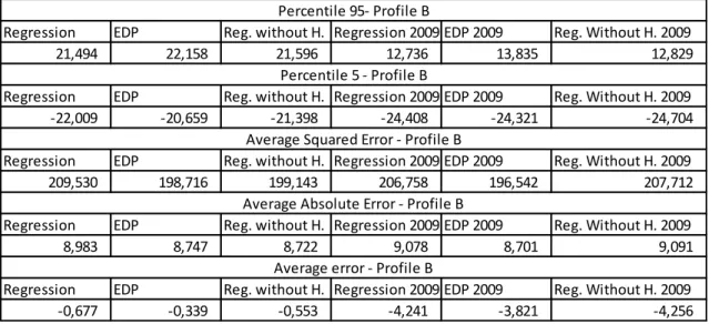
In table 5, it is shown that the lowest value of the 95th error percentile for the first years was the one from the new algorithm, with a value of 21.49, while for 2009, the algorithm with the lowest value is the new algorithm (12.74).

(16)

16

It is also shown that the algorithm that obtained a higher 5th error percentile value for the first years was the one from EDP (-20.66). As for the year of 2009, the highest value was registered by the EDP algorithm (-24.32).

We may also see that the algorithm with the lowest ASE for the first years was the one from EDP (198.72). For the year of 2009, the algorithm with the lowest ASE was EDP’s (196.54).

It also shows that the algorithm with the lowest AAE for the first years is the one of the new algorithm without heating (8.72). For the year of 2009, we can see that the algorithm with the lowest value of AAE was EDP’s (8.70).

As we can see in the last row, for the first years, the algorithm with the average error closest to 0 is the one from EDP (-0.34). About the 2009 estimations, the algorithm with the average error closest to 0 is also the one from the EDP (-3.82).

On these results, it is noticeable a better performance by the EDP algorithm for the years of 2006, 2007 and 2008. For the year of 2009, the criteria were favorable to the EDP algorithm.

Profile C

In table 6, it is shown that the lowest value of the 95th error percentile for the first years was the one from the new algorithm without heating and cooling, with a value of 2.86, while for 2009, the algorithm with the lowest value is the new algorithm without heating and cooling (2.42).

(17)

17

It is also shown that the algorithm that obtained a higher 5th error percentile value for the first years was the new algorithm (-3.63). As for the year of 2009, the highest value was registered by the EDP algorithm (-4.38)

We may also see that the algorithm with the lowest ASE for the first years was EDP’s (9.72). For the year of 2009, the algorithm with the lowest ASE was also EDP’s (17.90).

It also shows that the algorithm with the lowest average absolute error for the first years is the one of the new algorithm without heating and cooling (1.42). For the year of 2009, we can see that the algorithm with the lowest value of AAE was EDP’s (1.63).

As we can see in the last row, for the first years, the algorithm with the average error closest to 0 is the one from EDP (-0.12). About the 2009 estimations, the algorithm with the average error closest to 0 is again the one from the EDP’s algorithm (-0.23).

For this profile, there is again a slightly better performance of the EDP’s algorithm, when we compare the estimations for the years of 2006, 2007 and 2008, while for the year of 2009, the EDP’s algorithm still has better overall results.

As we may see, from these 3 previous tables, in 15 of the 30 tests, the new algorithm performed better than the new algorithm without temperature variables. If we take a closer look at the 2009 results (which are the ones that better simulate the usefulness of these algorithms), 10 out of 15 tests obtained better results with the new algorithm.

In the overall the algorithm from EDP’s outperformed the other two in almost every test, except in the percentiles, where in general, the new algorithms performed better. This overall performance of the EDP’s algorithm is understandable as it used a more detailed database and more detailed information when it was created.

(18)

18

4. Conclusion

From these results, there are some things that we may conclude. From these tests we were able to see that while the EDP’s algorithm presented a better performance in most of the averages criteria, the new algorithm along with the new algorithm without temperature variables tended to obtain better results on the percentiles criteria, which means that although the EDP’s algorithm has lower values of average errors, at the same time, it tends to have higher extreme errors. Additionally, we may also see that in the overall, the new algorithm performs better than the algorithm without temperature variables, especially for the year of 2009.

It is important to understand that the data used so that the new algorithm could be created, was way less detailed than the one used to create the EDP’s algorithm, since the sample used in this study only was able to provide average daily consumption, while the data used for the current algorithm provided the exact consumption for each day. Given the difference of data used in order to obtain both algorithms, it is understandable that the EDP’s algorithm obtained much better results in some of the criteria.

As a final remark, for future studies, it would be interesting to continue to try new ways of introducing temperature effects on electricity consumption algorithms, as this work shows that the introduction of these effects had improved results, when comparing with a similar algorithm without these variables. It would also be important to obtain a more detailed database and have access to the real daily consumptions, as it would certainly increase the inputs for the creation of the new algorithm. Furthermore, the temperatures gathered for this study were all from Lisbon, as the resources required to gather temperatures from all over the country would be much higher.

(19)

19

5. References

1 - Bessec, Marie; Fouquau, Julien. 2008. “The non-linear link between electricity

consumption and temperature in Europe: A threshold panel approach.” Energy

Economics Volume 30: 2705-2721;

2 - ERSE. 2011. Guia De Mediação, Leitura e Disponibilização De Ddados Para

(20)

20

Regression Statistics - Profile A

R Square 0,74 Adjusted R Square 0,74 Standard Error 0,03 Observations 1096

6. Appendices

6.1 Tables

Table 1 – Table with the regression data from the Profile A.

Table 2 - Table with the regression data from the Profile B.

Coefficients P-value Intercept 1,05 0,00 February -0,01 0,00 March -0,04 0,00 April -0,07 0,00 May -0,09 0,00 June -0,10 0,00 July -0,12 0,00 August -0,12 0,00 September -0,11 0,00 October -0,07 0,00 November -0,03 0,00 December 0,01 0,01 Heating 0,01 0,00 Regression - Profile A Coefficients P-value Intercept 1,09 0,00 February 0,00 0,63 March -0,03 0,00 April -0,08 0,00 May -0,13 0,00 June -0,18 0,00 July -0,21 0,00 August -0,21 0,00 September -0,19 0,00 October -0,13 0,00 November -0,04 0,00 December 0,04 0,00 Heating 0,01 0,00 Regression Profile B R Square 0,83 Adjusted R Square 0,83 Standard Error 0,04 Observations 1096

(21)

21 Table 3 - Table with the regression data from the Profile C.

Table 4 – Results from the criteria used to evaluate for the years of 2006,2007 and

2008, and then for 2009 – Profile A. Coefficients P-value Intercept 1,05 0,00 February 0,00 0,42 March -0,03 0,00 April -0,06 0,00 May -0,09 0,00 June -0,11 0,00 July -0,12 0,00 August -0,13 0,00 September -0,11 0,00 October -0,08 0,00 November -0,03 0,00 December 0,01 0,07 Heating 0,00 0,00 Cooling 0,01 0,00 Regression - Profile C

Regression EDP Reg. without H. Regression 2009 EDP 2009 Reg. Without H. 2009

16,318 16,334 16,238 13,888 14,574 14,062

-18,706 -18,847 -18,669 -20,911 -19,806 -20,983

187,025 192,140 186,820 219,490 150,102 224,613

7,168 7,272 7,166 7,604 7,486 7,603

-0,756 -0,748 -0,772 -1,818 -1,620 -1,820

Percentile 95 - Profile A

Percentile 5 - Profile A

Average Squared Error - Profile A

Average Absolute Error - Profile A

Average error - Profile A

R Square 0,68

Adjusted R Square 0,68

Standard Error 0,04

Observations 1096

(22)

22 Table 5 – Results from the criteria used to evaluate for the years of 2006,2007 and

2008, and then for 2009 – Profile B.

Table 6 – Results from the criteria used to evaluate for the years of 2006,2007 and

2008, and then for 2009 – Profile C.

21,494 22,158 21,596 12,736 13,835 12,829

-22,009 -20,659 -21,398 -24,408 -24,321 -24,704

209,530 198,716 199,143 206,758 196,542 207,712

8,983 8,747 8,722 9,078 8,701 9,091

-0,677 -0,339 -0,553 -4,241 -3,821 -4,256

Percentile 95- Profile B

Percentile 5 - Profile B

Average Squared Error - Profile B

Average Absolute Error - Profile B

Average error - Profile B

Regression EDP Reg. without H&C Regression 2009 EDP 2009 Reg. Without H&C 2009

2,889 2,870 2,864 2,429 2,670 2,421

-3,639 -3,732 -3,656 -4,814 -4,382 -4,806

9,885 9,715 9,858 18,863 17,901 18,835

1,424 1,499 1,422 1,702 1,629 1,703

-0,164 -0,118 -0,167 -0,442 -0,232 -0,445

Percentile 95 - Profile C

Percentile 5 - Profile C

Average Squared Error - Profile C

Average Absolute Error - Profile C

(23)

23 6.2. Figures

Figure 1 – Seasonality related to the months of the year.

Figure 2 – Temperature effects on electricity consumption – Profile A.

0 0,02 0,04 0,06 0,08 0,1 0,12 1 3 5 7 9 11 13 15 17 19 21 23 25 27 29 31

(24)

24 Figure 3 – Temperature effects on electricity consumption – Profile B.