Non-Identical Particle Femtoscopy in Models with Single Freeze-Out
Adam KisielFaculty of Physics, Warsaw University of Technology, ul. Koszykowa 75, 00-662 Warsaw, Poland
Received on 12 December, 2006
We present femtoscopic results from hydrodynamics-inspired thermal models with single freeze-out. Non-identical particle femtoscopy is studied and compared to results of Non-identical particle correlations. Special em-phasis is put on shifts between average space-time emission points of non-identical particles of different masses. They are found to be sensitive to both the spatial shift coming from radial flow, as well as average emission time difference coming from the resonance decays. The Therminator Monte-Carlo program was chosen for this study because it realistically models both of these effects. In order to analyze the results we present and test the methodology of non-identical particle correlations.
Keywords: Single freeze-out; Femtoscopy; Resonance contribution; Non-identical particle correlations
I. INTRODUCTION
The single freeze-out approach [1–3] originates from ther-mal models of heavy-ion collisions. It is based on therther-mal fits to particle yields and yield ratios, which are known to work well for RHIC collisions. These ratios are not sensitive to the underlying geometry of the collision, which is what is mea-sured by femtoscopy. The form of the freeze-out geometry must be postulated and should give the overall volume of the system, which is reflected in the absolute yields of particles, as well as the detailed shape of the emission region probed by two-particle correlations. We have postulated such a form of the freeze-out hypersurface which is motivated by hydrody-namics. It has been used to calculate femtoscopic observables, both for identical [4] and non-identical particles. The latter are especially interesting and are the focus of this work. They have been recently measured at SPS and RHIC [5–7]. There have been very few theoretical predictions for these observ-ables [5, 8]. They contain a crucial and unique piece of infor-mation - the difference between the average emission points of two particle types [9–13]. If the particles have different masses, we expect a spatial shift coming from the collective flow of matter. If the particles are of different type, we also expect a very different pattern of emission times, since many particles come from strong decays of resonances. Both of these shifts are interconnected in the measured average emis-sion point difference. Disentangling them is not a trivial task. Single freeze-out models with resonances are perfectly suited for it, as they include realistic modeling of both effects.
II. FEMTOSCOPY DEFINITIONS
In this work we will analyze correlation functions between non-identical particles. The femtoscopic correlation function is usually defined as:
C(q,K) =P
C 2(q,K) P0
2(q,K)
(1)
where P2C is the probability to observe two femtoscopically correlated particles at relative momentumq. P20is the prob-ability where the correlation between particles does not have
the femtoscopic component. Kis the average momentum of the pair. In heavy-ion experimentsP2C is usually constructed from pairs coming from the same event, while P20 is con-structed from pairs where each particle comes from a different event. The events are as close to each other in global charac-teristics as possible.
In theoretical models one should, in principle, generate par-ticles in such a way that they are already correlated due to their mutual and many-particle interactions. That is however usually computationally not possible. One then makes an as-sumption that the interaction between particles can be sepa-rated from the generation process and we write the most gen-eral form of the correlation function that can be used by mod-els:
C(q,K) =
S1,2(r∗,q,K)|Ψ(q,r∗)|2d4r∗
S1,2(r∗,q,K)d4r∗
(2)
wherer∗is the pair separation in the pair rest frame (PRF) and S1,2(r∗,q,K)is the pair separation distribution defined as:
S1,2(r∗,q,K) =
S1(x1,p1)S2(r∗−x2,p2) (3) δ(r∗−x1+x2)d4x1d4x2
andS(x,p)is the single-particle emission function provided by the model. For identical particlesS1≡S2andS1,2(r∗)is symmetric by definition, for non-identical particles it is not so andS1,2(r∗)is usually asymmetric. It is an important point which will be discussed later. We also note that the ordering of particles in the pair is important: S1,2(r)≡S2,1(−r). The Ψfunction will be discussed in the next chapter.
A. Wave-function of the pair
In Eq. 2 the amplitudeΨdescibes the change in the proba-bility to detect a pair of particles when they interact with each other. Generally, this (Bethe-Salpeter) amplitude depends on both spatial (r∗) and time(t∗)separation of the particle emit-ters in PRF. Usually, it can be approximated by the equal-time
(t∗=0)solutionΨ−k∗(r∗)of the scattering problem viewed
In this work we consider pairs of charged non-identical mesons and baryons. In this case the origin of femtoscopic correlations are Coulomb and strong interactions. However, for pion-kaon and pion-proton systems, as well as for same-charge kaon-proton system, the strong interaction is much weaker than Coulomb interaction at smallk∗. For the opposite charge kaon-proton system, there is a significant strong inter-action potential, which is interesting in it’s own right, how-ever its detailed study is beyond the scope of this paper. The strong interaction is not essential for our study, so we restrict our study to Coulomb interaction in same-charged pion-kaon, pion-proton and kaon-proton systems. Then:
Ψ(q,r∗)QC
2
= AC|F(−iη,1,iξ)|2 (4)
wherek∗is half of pair relative momentum in PRF,ACis the Gamow factor,F is the confluent hypergeometric function, η=1/k∗ac, ac is the pair Bohr radius andξ=k∗r∗+k∗r∗. Please note that the wave-function is calculated in the PRF.ac is 248.5f m, 222.6f mand 83.6f mfor pion-kaon, pion-proton and kaon-proton pair respectively.
III. NON-IDENTICAL PARTICLE CORRELATIONS
The correlation between a pair of non-identical particles arises from Coulomb and/or strong interaction. We will con-centrate on the Coulomb interaction, but our conclusions hold for strong interactions as well. We will discuss the specifics of the correlations for pairs of unlike particles, emphasizing the differences and similarities to traditional identical particle femtoscopy.
The correlation term (4) is calculated in the pair rest frame and depends on the relative momentumk∗, relative positionr∗ and the angleθ∗between the two. It needs to be emphasized that the low relative momentum in the pair rest frame, corre-sponds to closevelocities, but not momenta, in the laboratory frame. This is in contrast to identical particle interferometry. This also means that particles from very different momentum ranges are correlated, e.g. pion with velocity 0.7 has a mo-mentum of 0.137GeV, a close-velocity kaon has a momentum of 0.484GeV and a proton: 0.919GeV. In experiment this of-ten poses a problem, as one needs to have a large momentum acceptance to measure close-velocity pairs.
Looking in detail at the hypergeometric function F from (4):
F=1+r∗(1+cosθ∗)/aC+... (5) one notices an important feature of|Ψ|2, namely that it is not symmetric with respect to the sign of cosθ∗. For same sign particlesAcis less than 1.0 andF is above 1.0, but since the correlation effect must be negative,Ac|F|2<1. For a given
k∗andr∗one can have two cases: in one cosθ∗<0, for the other cosθ∗>0. The former will have alargercorrelation ef-fect (sinceFis smaller and cannot overcomeAc) and the latter will have asmallercorrelation effect. This asymmetry in the correlation effect can be understood with the help of a simple picture: negative cosθ∗means thatk∗andr∗are anti-aligned,
which means that at first the particles will fly towards each other before they fly away, spending more time close together and thus developing a larger correlation. A positive cosθ∗ means they will fly away immediately, having no time to in-teract. This asymmetry is an intrinsic property of the Coulomb interaction and is also present for identical particles. However in that case the wave-function symmetrization requires one to add a second term to (4) which has the same asymmetry with the opposite sign, so that the overall asymmetry is zero, as it must be.
If we were somehow able to divide pairs in two groups -one in whichcosθ∗>0 and the other in whichcosθ∗<0 one would obtain two different correlation functions, out of which the latter would show a stronger correlation effect. Ob-viously we cannot select pairs based on theθ∗angle, as it is not measured. However we do have one angle on which we can select - the angleΨbetween pair velocityvand pair rel-ative momentumk∗. In the transverse plane cosΨ>0 means thatkout∗ >0. We also notice that in the transverse plane
Ψ=θ∗+φ, (6)
whereφis the angle between the pair velocityvand the rel-ative positionr∗. This angle is not measured as accurately. One can also show that when one averages over all possible positions ofr∗one can write [14]
signcosΨ=signcosθ∗signcosφ. (7) One can then propose a measurement: to divide pairs into two groups, one withk∗out >0 ≡cosΨ>0 and the other with k∗out <0≡cosΨ<0. Then one constructs two correlation functionsC+ andC− from the two groups. If one observes that|C+−1|/|C−−1.0|>1.0 it can only happen ifcosφ<0 as can be seen from Eq. (7). In other words this can happen only if the average emission points of two particle species are, on the average, separated in the direction of the pair velocity, and this separation is anti-aligned with the velocity. By the same reasoning, if|C+−1|/|C−−1.0|<1.0 this separation is aligned with the pair velocity. Let us restate the conclusion of this paragraph: using the fact that the correlation effect is asymmetric with respect to the sign ofcos(θ∗)and the mea-sured angleΨ, we can tell whether an average emission po-sition of two different particle species is the same or not, and if it is not, is the difference is the same or opposite to the di-rection of pair velocityv. More quantitative analysis shows, that the double ratioC+/C−is also monotonously dependent on the value of this shift between particles, so the magnitude of the shift can be inferred from it. This is a unique feature of non-identical particle correlations, as such information cannot be obtained from any other measurement.
A simple formula can be written for the behavior of the double-ratio at lowk∗[11]:
lim
k∗→0C+/C−=1+2r ∗
i/aC (8)
usually suffers from low statistics and two-track separation problems.
The above consideration has been performed for the pair rest frame. Experimentally, however, one would like to learn something about the source itself, which requires the knowl-edge of the source in its rest frame. In symmetrical collisions in collider experiments (which is what we will consider later in the manuscript) we can assume that the source frame co-incides with the laboratory frame. One can write a simple formula for the relative separation in pair rest framer∗ as a function of the pair separation in the source framer:
r∗out = γt(rout−βt∆tL)
r∗side = rside
rlong∗ = γl(rlong−βl∆t)
∆tL = γl(∆t−βlrlong) (9) where thelongdirection is defined as the one parallel to the velocity of the colliding nuclei, out as parallel to the pair velocity in the transverse direction, andside as perpendic-ular to the other two. The pair velocities are βl =pl/E, γl=1/
1−β2
l,βt=p⊥/m⊥,γt=1/
1−β2
t. One can see that the average shift inr∗outmay mean non-zero average spa-tial shiftrout, non-zero average emission time difference∆tor a combination of the two.
IV. THERMINATOR
The Therminator program [15] is the numerical implemen-tation of the single freeze-out model [1–3]. It includes all particles listed by the Particle Data Group [16]. We use the version of the model based on the blast-wave type parame-trization, which is hydrodynamics-inspired [8]. Therefore our model includes the effects of radial flow, which is appar-ent, e.g., in themT dependence of the pion “HBT radii” [4]. This is an important feature, as the space-momentum corre-lation coming from radial flow is one of the origins of sion asymmetries between various particle species. The emis-sion function is changed slightly from the veremis-sion described in [15]. A quasi-linear velocity profile as a function ofρis added. The freeze-out hypersurface is then defined as:
˜
τ=τ=const, vr=tanhα⊥=
ρ/ρmax
vT+ρ/ρmax
(10)
whereτ,ρmaxandvT are parameters of the model. The quasi-linear velocity profile has the desired features - it is zero for ρ=0, is almost linear for reasonable values ofvT, and cannot go higher than 1.0. The emission function is then:
dN
dydϕp⊥d p⊥dαdφρdρ
= τ
(2π)3m⊥cosh(α−y)× (11)
exp
βm⊥cosh(α−y)−p⊥vrcos(ϕ−φ)
1−v2 r
−βµ
±1 ,
where(ρ,φ)is the transverse emission point in radial coordi-nates, αis the space-time rapidity of the emission point, y
is the particle rapidity,(pT,ϕ)is the particle’s transverse mo-mentum in radial coordinates, andmT is its transverse mass. The inverse temperatureβandµ, the particle-specific chemi-cal potentials, are also parameters of the model.
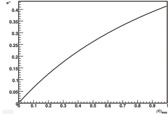
The fit to STAR Collaboration data [17] has been performed with this model and the following values of the parameters were found to best reproduce the observed pion and kaon spectra in central AuAu collisions:τ=8.55 fm,ρmax=8.92 fm,a=−0.5,vT =1.41. The negative value of thea para-meter means that the freeze-out hypersurface has a negative slope (an anti-correlation) in theρ−tplane, or in other words the freeze-out occurs outside-in [4]. The thermodynamic pa-rametersTandµwere the same as in [4]. The velocity profile for these parameters is shown in Fig. 1. The average velocity is 0.31.
max
ρ
/
ρ
0 0.1 0.2 0.3 0.4 0.5 0.6 0.7 0.8 0.9 1
r
v
0 0.05 0.1 0.15 0.2 0.25 0.3 0.35 0.4
FIG. 1: Radial velocity profile for the parameters used in this study.
emission time [fm]
0 10 20 30 40 50
emission probability P(t)
-5
10
-4
10
-3
10
-2
10
-1
10
FIG. 2: (Color online) Probability to emit a pion (green triangles), kaon (blue squares) and proton (red circles) as a function of time.
TABLE I:Average emission times from Therminator
Particle species Average emission time
pion 12.3f m/c
kaon 10.7f m/c
The simulation proceeds as follows. First, using a Monte-Carlo integration procedure as a particle generator, all parti-cles (stable and unstable) are generated according to the emis-sion function (11). Each particle is given an emisemis-sion point on the freeze-out hypersurface and a momentum. Then, all unstable particles decay after some random time dependent on their width. They propagate to the decay point, and this point is then taken as the space-time origin of the daughter particles. Two- and three-particle decays are implemented. The process is repeated for cascade decays, until only stable particles remain. While each particle has its emission point either on the freeze-out hypersurface (we call such particles primordial) or at the decay point of the heavier resonance, the full history of decays can be reconstructed from the output files. This treatment of resonance propagation and decay is of crucial importance for non-identical particle correlations. It introduces delays in emission time, which are different for different particle species. It depends on the number of res-onances that decay into the particle of interest, their widths and velocities. An illustration can be seen on Fig. 2. The Monte-Carlo procedure we used is the most efficient way of studying it, more precise results can only be obtained by us-ing a full-fledged hadronic rescatterus-ing model. In our work hadronic rescattering is not taken into account, which is one of the simplifications assumed in the single freeze-out model.
A. Calculating the correlation function
It is possible to use Eq. 2 to obtain the model correlation function. The integral is calculated numerically. One takes particles generated by Therminator. Then one combines them into pairs and creates two histograms - in one of them one stores the|Ψ|2of the pair (4), in the other - unity for each pair. The result of the division of the two histograms is the average correlation effect in each bin, which is the correlation func-tion per Eq. (2). This is the so-called “two-particle weight” method of calculating the correlation function from models. It is the only one which takes into account the two-particle Coulomb interaction exactly, a feature which is necessary for our study. In this procedure each pair is treated separately, as one goes to the pair rest frame (different for each pair) as the calculation of theΨis done most naturally in this system.
V. ASYMMETRY ANALYSIS
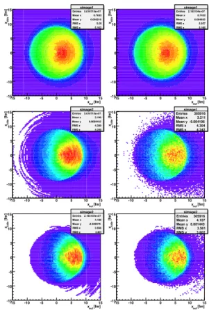
In section III it was shown that non-identical particle cor-relations are sensitive to the shifts between average emission points of different particle species. However, we have not dis-cussed if and how such asymmetries could arise. In Fig. 3 the average emission points of pions, kaons and protons from THERMINATOR where shown for pairs which have similar velocity, pointing horizontally to the right. One sees that the average emission points of pions, kaons and protons isnotthe same in theoutdirection, while it is 0 for the side direction for all of them. One can also see that the average size of the emis-sion region is decreasing with particle mass, a known effect of
[fm] out x -15 -10 -5 0 5 10 15
[fm] side x -15 -10 -5 0 5 10
15 Entries 5.016718e+07simage1 Mean x 0.7633 Mean y 0.005216 RMS x 5.05 RMS y 5.162 simage1 Entries 5.016718e+07 Mean x 0.7633 Mean y 0.005216 RMS x 5.05 RMS y 5.162
[fm] out x -15 -10 -5 0 5 10 15
[fm] side x -15 -10 -5 0 5 10
15 Entries 2.193154e+07simage1 Mean x 0.7422 Mean y 0.004935 RMS x 5.057 RMS y 5.166 simage1 Entries 2.193154e+07 Mean x 0.7422 Mean y 0.004935 RMS x 5.057 RMS y 5.166
[fm] out x -15 -10 -5 0 5 10 15
[fm] side x -15 -10 -5 0 5 10
15 Entries 5.016718e+07simage2 Mean x 3.199 Mean y 0.0009162 RMS x 4.309 RMS y 4.349 simage2 Entries 5.016718e+07 Mean x 3.199 Mean y 0.0009162 RMS x 4.309 RMS y 4.349
[fm] out x -15 -10 -5 0 5 10 15
[fm] side x -15 -10 -5 0 5 10
15 Entries simage1305916 Mean x 3.211 Mean y -0.004106 RMS x 4.304 RMS y 4.342 simage1 Entries 305916 Mean x 3.211 Mean y -0.004106 RMS x 4.304 RMS y 4.342
[fm] out x -15 -10 -5 0 5 10 15
[fm] side x -15 -10 -5 0 5 10
15 Entries 2.193154e+07simage2 Mean x 4.108 Mean y -0.009375 RMS x 3.556 RMS y 3.801 simage2 Entries 2.193154e+07 Mean x 4.108 Mean y -0.009375 RMS x 3.556 RMS y 3.801
[fm] out x -15 -10 -5 0 5 10 15
[fm] side x -15 -10 -5 0 5 10
15 Entries simage2305916 Mean x 4.107 Mean y 0.001443 RMS x 3.561 RMS y 3.802 simage2 Entries 305916 Mean x 4.107 Mean y 0.001443 RMS x 3.561 RMS y 3.802
FIG. 3: (Color online) Distribution of emission points of pions (up-per plots), kaons (center plots) and protons (lower plots) versus pair-wise out and side directions. Left and right side are emission points of the same particle from different system, but for the same pair ve-locity range (for pions: left -πK, right -πp, for kaons: left -πK, right -K p, for protons: left -πp, right -K p.
radial flow, usually referred to as “mT scaling” of HBT radii.
The shift that we observe is also a direct but distinctly dif-ferent consequence of radial flow present in our simulation. The mt dependence of the average emission point has been
discussed in detail in [5] and the formula for the longitudinal boost-invariant hydrodynamic model (similar to the one used in this work) has been given:
x=r0
β0βt β2
0+T/mt
(12)
wherer0is the radius of the system,βtis the transverse
so the emission points will tend to be concentrated near the edge of the system, in the direction of emission. For pions on the other hand, there is almost no correlation between the two directions, so they are emitted from the whole source. The ef-fect is clearly seen in the figure, as a difference between mean emission points in the “out” direction:
routπp=xπout−xoutp (13) This is the spatial shift between particles in the source frame. Measuring it is the main goal of non-identical particle fem-toscopy. Observing such a shift in the experiment would be direct evidence of the collective behavior of matter, which is one of the necessary conditions to claim the discovery of the quark-gluon plasma.
One must remember that the asymmetries measured in the correlation function are averaged over the source. Therefore, the connection between a shift in the laboratory frame and in the pair rest frame is:
rout∗ =γ(rout−β∆t) (14)
TABLE II:Average space shifts from Therminator
βtof the pair rπK rπp rK p
0.35 - 0.5 -1.9 fm -2.5 fm -0.6 fm
0.5 - 0.65 -2.4 fm -3.4 fm -0.9 fm 0.65 - 0.8 -2.9 fm -3.9 fm -1.1 fm 0.8 - 0.95 -3.0 fm -4.3 fm -1.2 fm
TABLE III:Average time shifts from Therminator
βtof the pair ∆tπK ∆tπp ∆tK p
0.35 - 0.5 3.8 fm/c 6.2 fm/c 2.3 fm/c 0.5 - 0.65 3.6 fm/c 5.7 fm/c 2.1 fm/c 0.65 - 0.8 3.2 fm/c 5.1 fm/c 1.9 fm/c
0.8 - 0.95 2.6 fm/c 4.2 fm/c 1.5 fm/c
From Eq. (9) one sees that the measurable shiftr∗out is a combination of the spatial shiftrout, and the emission time shift∆t. The former effect is of special interest and has been studied in detail in [8]. However, the effect of time differ-ence has not been adequately studied so far. The Therminator model has been chosen to perform this task, because it in-cludes both effects in the same calculation in a self-consistent way. Fig. 2 shows the probability to emit a pion, a kaon or a proton at a given time. One sees that the average emission times of this particle species, listed in Tab. I, are different in the laboratory frame. This will affect the observed asymme-tries.
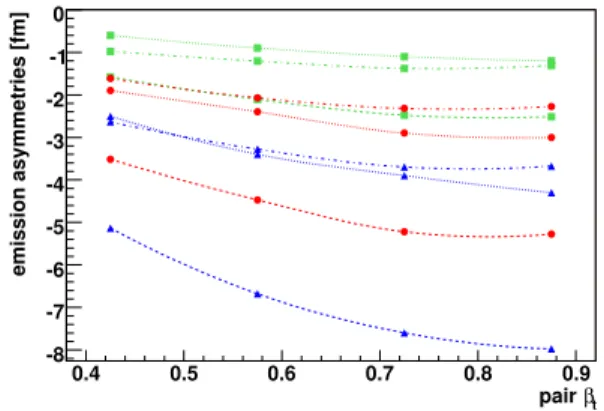
In Fig. 4 one can see the components of the emission asym-metries in the laboratory frame, obtained directly from the emission functionsS1,2. The time and space components for all considered systems are compared. They are of the same or-der for all systems. The overall asymmetry is the combination of the two.
t β pair
0.4 0.5 0.6 0.7 0.8 0.9
emission asymmetries [fm]
-8 -7 -6 -5 -4 -3 -2 -1 0
FIG. 4: (Color online) Components of the average shift between particle species in the laboratory frame. The dotted line is the space component, the dash-dotted line is the time component, and the dashed line is the full asymmetry. Red circles are for theπK sys-tem, blue triangles are forπp, green squares are forK p.
A. Obtaining femtoscopic information
The correlation function for non-identical particles is given by Eq. (2). In order to obtain femtoscopic information from the experimental correlation function one needs to perform a fit procedure. In traditional HBT measurement the integral analog to Eq. (2) can be performed analytically to obtain a simple fit function. It is not possible for the general case of non-identical particles, where the following procedure must be applied. Usually it is assumed that the emission function factorizes into space and momentum components. A form of the spatial emission function is then postulated:
S(r)≈exp
−(rout−µout) 2+r2
side+rlong2 2R2
(15)
B. Sum rule for shifts between different particle species
If we have three different particle species, we have three average emission point shifts that we can measure: µπK,µπp andµK p. However, if we take the same group of e.g. pions forπ−K correlations and π−p correlations (and similarly the same group of kaons and protons), we might expect that a simple sum rule holds:
µπp=µπK+µK p (16) and only two of the shifts are independent.
Non-identical particles are correlated if they have close ve-locities. If we select pairs of particles with some pair velocity, we expect that the correlated particles themselves also have velocities in this range. Therefore if we compare pions that form theπ−K correlation in the pair βt range between 0.5 and 0.65, and pions from theπ−p correlation in the same pairβt range we may assume that these are the same pions (providing that we construct the correlation functions from the same events). That shows that pairβtis the correct variable to select on, when studying momentum dependence of the fem-toscopic parameters from non-identical particle correlations. It also shows that we should indeed expect the sum rule (16) to hold separately in eachβtbin.
C. Two-particle versus single particle sizes
The size of the two-particle source is a combination of the individual single-particle source sizes:
σπK =
σ2
π+σ2K
σπp =
σ2
π+σ2p
σK p = σ2
K+σ2p (17)
whereσis a width of a gaussian fitted to the corresponding emission function (either single- or two-particle). One can immediately see that the sizes are not independent, similar to the shifts. One can also use the combination of the measured two-particle source sizes to obtain the single particle sizes:
σπ =
σ2
πK+σ2πp−σ2K p 2
σK =
σ2
πK−σ2πp+σ2K p 2
σp =
−σ2
πK+σ2πp+σ2K p
2 (18)
They can then be compared to single-particle source sizes obtained from regular identical particle interferometry to see whether the size of the system is described self-consistently.
) * k* [GeV/c] out sign(k* -0.08 -0.06 -0.04 -0.02 0 0.02 0.04 0.06 0.08
C(k*)
0.82 0.84 0.86 0.88 0.9 0.92 0.94 0.96 0.98 1
FIG. 5: (Color online) Correlation functions for pion-kaon (red), pion-proton (yellow) and kaon-proton (blue) for pairs with velocity between 0.5 and 0.65. The lines are fits to the correlation function.
VI. RESULTS AND DISCUSSION
The analysis of the correlation functions for pion-kaon, pion-proton and kaon-proton systems has been performed based on the Therminator model and the two particle weight method, described in the previous paragraphs. Examples of the obtained correlation functions are shown in Fig. 5. As ex-pected for like-sign pairs they go below unity at lowk∗. The correlation effect is the smallest for pion-kaon and largest for kaon-proton due to the difference in the Bohr radii of the pairs. It is a fortunate coincidence, as for kaon-proton one expects to have the smallest statistics in the experiment, but due to a large correlation effect the measurement should be doable for a data sample similar to the one in which pion-kaon measure-ment is possible.
k* [GeV/c] 0 0.01 0.02 0.03 0.04 0.05 0.06 0.07 0.08
C+/C-0.85 0.9 0.95 1 1.05 1.1 1.15
FIG. 6: (Color online) Double ratios for kaon (red), pion-proton (yellow) and kaon-pion-proton (blue) for pairs with velocity be-tween 0.5 and 0.65. The lines are double ratios calculated from the fits to the correlation function.
shown in Fig. 3, and with emission time differences coming from resonance decays, shown in Fig. 2 and Tab. III.
The correlation functions have been fitted using the numer-ical Monte-Carlo procedure described in Sect. IV. Fig. 5 shows the resulting best-fit functions as solid lines. The fit is performed simultaneously to the positivekout∗ and negative k∗out part of the correlation function. The lines in Fig. 6 are simply the two parts of the fit function from Fig. 5 divided by each other, they are not fit independently.
β pair
0.4 0.5 0.6 0.7 0.8 0.9
[fm]
σ
R,
5 6 7 8 9 10
β pair
0.4 0.5 0.6 0.7 0.8 0.9
, <r> [fm]
µ
-10 -8 -6 -4 -2 0
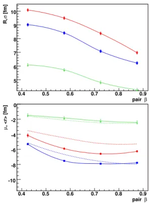
FIG. 7: (Color online) Parameters of the non-identical particle sources from fits. In the upper panel source size is shown, in the lower - shift between mean emission points in the direction of pair transverse momentum. Red circles are for pion-kaon, blue squares for pion-proton, green triangles for kaon-proton. Dashed lines are input overall asymmetries from Fig. 4.
The results of the fit are shown in Fig. 7. We find that the size of the emitting system decreases with pair velocity for all considered pair types. This is consistent with the “mT
scaling” of the HBT radii observed in the identical particle femtoscopy calculations. The shifts between various particle species have an expected ordering - the larger the mass dif-ference, the larger the shift. This means that for all observed systems the lighter particle is emitted, on the average, closer to the center and/or later than the heavier one. It also means that time differences do not change the qualitative behavior of the observed asymmetries. However, consulting Tab. III and Fig. 4, one can see that they do contribute to the ob-served asymmetry. The dashed lines in Fig. 7 show the overall asymmetry from Fig. 4 as predicted directly from the emission functionsS1,2(r)from the model. The agreement in absolute values and in the general trends between them and the final fit values is within 1.0f m.
This is of crucial importance for the experiment. It means that by performing an advanced fit of all three combinations of non-identical particle correlation functions one can indeed infer the properties of the underlying two-particle emission functions, and therefore obtain a new, unique piece of infor-mation about the dynamics of the collision.
t β pair
0.4 0.5 0.6 0.7 0.8 0.9
[fm]
K p
µ
-
K
π
µ
- p
π
µ
-1.5 -1 -0.5 0 0.5 1 1.5
FIG. 8: (Color online) Test of the sum rule of mean shifts between various particle types.
One can also test the validity of the sum rule (16). The test using the fit values from Fig. 7 is shown in Fig. 8. One can see that the rule is valid for smaller pair velocity and holds only approximately for larger velocities. This should be com-pared to results in Tab. II, where the shifts obtained from the separation distributions themselves follow the sum rule with the accuracy of 0.1f m. Also, one can expect deviations on the order of the differences between the input and fitted val-ues of the shift shown in Fig. 7. One can see that within these systematic limits the agreement is acceptable. This is another important conclusion for the experiment. If shifts between all three combinations are measured in the comparable pair ve-locity window one expects the sum rule for the shifts (16) to hold. It can be used as a quality check on the data.
particle m
0 0.2 0.4 0.6 0.8 1 1.2 1.4 1.6 1.8 2
Source size [fm]
0 1 2 3 4 5 6 7 8
FIG. 9: (Color online) Single particle source sizes obtained from non-identical particle correlation fits, according to (18). Red circles are pions sizes, blue squares - kaon, green triangles - proton. Open circles are sizes obtained from identical-particleπcorrelations.
the expected “mT scaling” for all particle species. Therefore an experiment can extract the information not only about the asymmetries of emission but also about the size of the system. The comparison between the size estimates obtained from non-identical particle correlations and “HBT radii” obtained from identical pion interferometry was done. Both sizes for pions are consistent with each other. One must remember that in the case of Therminator model, the obtained source func-tions exhibit large long-range non-gaussian tails [4]. On the other hand, both identical and non-identical femtoscopic sizes were obtained assuming a perfect gaussian source. Both of these measures can be sensitive to long-range tails in a differ-ent way, so the comparison must be done with caution.
VII. SUMMARY
We have presented the first complete set of calculations of non-identical particle correlations from the single freeze-out models with complete treatment of resonances. Non-identical particle femtoscopy method was shown to be sensitive to both the size and emission asymmetries in the system. The ob-served effects have been shown to be under control both quali-tatively and quantiquali-tatively. The method to extract femtoscopic information from such correlation functions have been pre-sented and employed to the “pseudo-experimental” functions obtained from the model. The results of the fit have been shown to be in agreement with the characteristics of the input
source. Several consistency checks on the experimental data have been proposed and their validity tested. A method to test the consistency of identical and non-identical femtoscopy results has also been proposed.
The femtoscopic analysis of non-identical particle correla-tions has shown that the emission asymmetries between pions, kaons and protons are expected to occur in heavy-ion colli-sions. Spatial asymmetry coming from radial flow was ob-served. Time asymmetry coming from resonance propagation and decay was also estimated and found to be on the order of the space asymmetry in the laboratory frame and in the same direction for all tested systems. Therefore a realistic and self-consistent estimate of the two effects has been given for the first time. Consistency between identical and non-identical femtoscopic sizes was tested and found to be within 1.0 fm.
Predictions for both the size of the system as well as emis-sion asymmetry have been given for central AuAu colliemis-sions for pion-kaon, pion-proton and kaon-proton correlations.
Acknowledgements
This work was supported by Polish Ministry of Science and Higher Education, grants no. 0395/P03/2005/29 and 134/E-365/SPB/CERN/P-03/DWM 97/2004-2007. I would like to thank Prof. W. Broniowski and Prof. W. Florkowski for very fruitful discussions.
[1] W. Florkowski, W. Broniowski, and M. Michalec, Acta Phys. Polon. B33, 761 (2002) [arXiv:nucl-th/0106009].
[2] W. Broniowski and W. Florkowski, Phys. Rev. Lett.87, 272302 (2001) [arXiv:nucl-th/0106050].
[3] W. Broniowski, A. Baran, and W. Florkowski, AIP Conf. Proc.
660, 185 (2003) [arXiv:nucl-th/0212053].
[4] A. Kisiel, W. Florkowski, and W. Broniowski, Phys. Rev. C73, 064902 (2006) [arXiv:nucl-th/0602039].
[5] R. Lednicky, Proc. CIPPQG’01, Palaiseau, France, Phys. Atom. Nucl.67, 72 (2004) [arXiv:nucl-th/0112011].
[6] C. Blume et al., Nucl. Phys. A 715, 55 (2003) [arXiv:nucl-ex/0208020].
[7] J. Adams et al. [STAR Collaboration], Phys. Rev. Lett. 91, 262302 (2003) [arXiv:nucl-ex/0307025].
[8] F. Retiere and M. A. Lisa, Phys. Rev. C70, 044907 (2004) [arXiv:nucl-th/0312024].
[9] R. Lednicky, V.L. Lyuboshitz, Yad. Fiz.35, 1316 (1982) (Sov. J. Nucl. Phys.35, 770 (1982); Proc. Int. Workshop on Paricle Cor-relations and Interferometry in Nuclear Collisions, CORINNE 90, Nantes, France 1990 (ed. D. Ardouin, World Scientific 1990) p. 42; Heavy Ion Physics3, 1 (1996).
[10] R. Lednicky, V. L. Lyuboshits, B. Erazmus, and D. Nouais,
Phys. Lett. B373, 30 (1996).
[11] S. Voloshin, R. Lednicky, S. Panitkin, and N. Xu, Phys. Rev. Lett.79, 4766 (1997) [arXiv:nucl-th/9708044].
[12] R. Lednicky, “Finite-size effects on two-particle production in continuous and discrete spectrum”, arXiv:nucl-th/0501065. [13] A. Kisiel, “Non-identical particle femtoscopy in heavy-ion
col-lisions,” AIP Conf. Proc.828, 603 (2006).
[14] A. Kisiel, “Studies of non-identical meson-meson correlation at low relative velocities in relativistic heavy-ion collisions regis-tered in the STAR experiment”, PhD Thesis, Warsaw Univeristy of Technology (2004).
[15] A. Kisiel, T. Taluc, W. Broniowski, and W. Florkowski, Com-put. Phys. Commun.174, 669 (2006) [arXiv:nucl-th/0504047]. [16] S. Eidelmanet al.[Particle Data Group], “Review of particle
physics,” Phys. Lett. B592, 1 (2004).
[17] J. Adams et al.[STAR Collaboration], Phys. Lett. B 616, 8 (2005) [arXiv:nucl-ex/0309012].