Bol. Ciênc. Geod. vol.18 número3

(1)

Bol. Ciênc. Geod., sec. Artigos, Curitiba, v. 18, no_{3, p.378-396, jul-set, 2012.}

APPLICATIONS OF VORONOI AND DELAUNAY

DIAGRAMS IN THE SOLUTION OF THE GEODETIC

BOUNDARY VALUE PROBLEM

Aplicações de Diagramas de Voronoi e Delaunay na Solução do Problema Geodésico do Valor de Contorno

C. A. B. QUINTERO1 I. P. ESCOBAR2 C. F. Ponte-NETO1

1

Observatório Nacional, Ministério da Ciência e Tecnologia, Rio de Janeiro, Brazil

2

Departamento de Engenharia Cartográfica, Universidade do Estado do Rio de Janeiro, Rio de Janeiro, Brazil

bonilla@on.br; irisescobar@gmail.com; cosme@on.br

ABSTRACT

Voronoi and Delaunay structures are presented as discretization tools to be used in numerical surface integration aiming the computation of geodetic problems solutions, when under the integral there is a non-analytical function (e. g., gravity anomaly and height). In the Voronoi approach, the target area is partitioned into polygons which contain the observed point and no interpolation is necessary, only the original data is used. In the Delaunay approach, the observed points are vertices of triangular cells and the value for a cell is interpolated for its barycenter. If the amount and distribution of the observed points are adequate, gridding operation is not required and the numerical surface integration is carried out by point-wise. Even when the amount and distribution of the observed points are not enough, the structures of Voronoi and Delaunay can combine grid with observed points in order to preserve the integrity of the original information. Both schemes are applied to the computation of the Stokes’ integral, the terrain correction, the indirect effect and the gradient of the gravity anomaly, in the State of Rio de Janeiro, Brazil area.

Keywords: 2-D tessellation; Delaunay Triangulation; Voronoi Cells; Geodesy;

(2)

Quintero, C. A. B. et al.

3 7 9

RESUMO

Este trabalho apresenta as estruturas de Voronoi e Delaunay como ferramentas de discretização a serem usadas na integração numérica de superfícies com o objetivo de resolver problemas computacionais geodésicos, quando no integrando a função não é analítica. No enfoque de Voronoi, a região de trabalho é particionada em polígonos, os quais contêm um ponto por polígono o que faz desnecessária a interpolação. No enfoque de Delaunay, os pontos observados são os vértices de um triangulo, e o valor da célula é o resultado da interpolação sobre o triangulo pelo seu baricentro. Se a quantidade de pontos observados e a sua distribuição são adequadas, a interpolação em grade não é necessária, e a integração é levada a cabo ponto a ponto. Mesmo quando a quantidade e distribuição dos pontos observados não são suficientes, as estruturas de Voronoi e Delaunay podem combinar grade com pontos observados a fim de preservar a integridade da informação original. Ambos os enfoques são aplicados ao cálculo da integral de Stokes, da correção de terreno, do efeito indireto, e do gradiente da anomalia da gravidade na região do estado de Rio de Janeiro, no Brasil.

Palavras-chave: Tesselação 2-D; Triangulação de Delaunay; Celulas de Voronoi;

Geodésia; Integral de Stokes.

1. INTRODUCTION

(3)

Applications of Voronoi and Delaunay diagrams in the solution of...

3 8 0

‘nodes’ separation, which are inherent to the spatial data distribution (e.g., GOLDEN SOFTWARE, 1999). In the worst case, it may produce spurious data that may lead to an inaccurate geoid. Also, different gridding methods provide different interpretations of the data because the grid node values are computed by different algorithms.

In this work, the discretization by means of Voronoi and Delaunay structures (AURENHAMMER, 1991; WATSON, 1981) is used to the computation of the Stokes’ integral, terrain correction, indirect effect and gradient of the Helmert anomaly. Both approaches are reported in Santos and Escobar (2006, 2010). Genuine data are used and preserved if they have such a spatial distribution that does not require filling blank areas with interpolated data. In spite of a natural “smoothing” due to the data distribution, Voronoi and Delaunay schemes avoid the “synthetic” smoothing due to an interpolation step. Alternatively, if the original data are not sufficient, they can still be preserved in combination with a grid used to fill the blank areas. In Voronoi scheme, the target area is subdivided into a unique set of convex and adjacent polygonal cells, in which each one holds an original data point. In Delaunay scheme, the area is tessellated into contiguous triangular cells (triangulated irregular network - TIN). Mean values are locally interpolated for the barycenter (centroid) from respective triangles’ vertices and remains enclosed to each cell (GOLDEN SOFTWARE, 1999).

2. THE TESSELLATION METHOD

Several authors have investigated Voronoi and Delaunay structures, their properties and applications in many different scientific fields. Those structures are used in the analysis of elements that have to be partitioned into contiguous domains called “natural neighbors”. This term was coined by mathematicians, when noticing the frequent instances of those relationships found in the nature. Many geometric natural shapes tend to be organized into Voronoi-like figures, such as the formed surface layer of mud that has dried and contracted, or the tessellated bony shell of some turtles and tortoises.

In gravimetry, Delaunay triangulation has been used to model the topography for terrain corrections computation, in which the relief is represented by triangular prisms (RUPERT, 1988). Lehmann (1997) used a triangulation structure to model equilateral spherical triangles for the evaluation of geodetic surface integrals.

A Voronoi diagram is also referred to as the Dirichlet tessellation, and might be viewed as a geometric complement (a duality) to Delaunay triangulation (AURENHAMMER, 1991; TSAI, 1993). The polygon vertices are associated with Delaunay triangles by the same construction rule – the circumcircle criterion or the Delaunay criterion (TSAI, 1993).

2.1. Construction of Delaunay Triangulation and Voronoi Diagram

(4)

3 8 1 1b). Given a set of n distinct points in S, so that

n

>

m

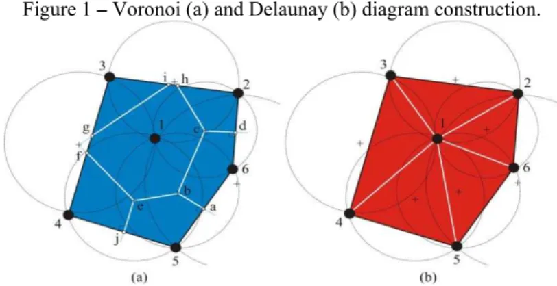
, every circumcircle associated with the triangles must contain no other points inside it. Whereas k points belonging to the perimeter of the area (peripheral points), the number of triangles generated is equal to 2(n - 1)- k. The interesting property of this structure (the approximated equiangular form) indicates that minimum angles are maximized and maximum angles are not minimized, which is an advantage over any triangulation of the same set of points. By Delaunay criteria, any triangulation with no obtuse angles has to be a Delaunay triangulation. According to Aurenhammer (1991), a triangulation without extreme angles (or "compact") is desirable, especially in methods of data interpolation. Additionally, in graphical computation the equiangular property is a need that provides the best visualization for displaying figures.

The vertices in Delaunay triangulation are all and only the n points of S, and its circumcenters are the actual Voronoi polygon vertices, or Voronoi polytopes (Figure 1a). The remaining circumcenters not satisfying the ‘empty circumcircle criterion’ are discarded from the construction.

The automatic contouring of the points is according to the triangulation algorithm by D.F. Watson (RUPERT, 1988), which was modified to include the Voronoi polygons’ computation, in which the topological data structures set up the relations between data points, edges and Delaunay triangles. The algorithm implicitly ensures a closed bounding area perimeter (the convex hull), but it does not preserve its outer limits because this information is not required for the triangulation.

Figure 1 – Voronoi (a) and Delaunay (b) diagram construction.

A Voronoi diagram is a partition

π

i of space S into n polygons, so that each

(5)

Bol. Ciê 3 8 2

{

i

=

π

where T halfwa rise t (AURE and an of the space i T the sam vertice in the constru same. 3. APP A as the in Gui compu de Jan betwee applied Helme

ênc. Geod., sec. A

{

x

∈

S

,

i

=

1

d is the point The Voronoi s

ay between ea to convex ENHAMMER ny vertex is eq region. By is partitioned The topologica

me as in Del es and polygo

Delaunay tria uctions is per

PLICATION

A comprehens main Bounda marães and B ute the Stokes neiro State (an

en 0 – 2,600 d to the comp ert gravity ano

App

Artigos, Curitiba,

i

x

d

n

(

,

K

-to-vertex Euc structure is un ach pair of site polygons, e R, 1991). Als quidistant to e

construction, into exactly i al data structu launay triang ns edges is ne angulation. Ad rformed to ve

N OF VORON

sive approach ary Value Prob Blitzkow (2011 ’ integral for t nd nearby reg 0 m (Figure 2

putation of ter omaly.

Figure 2 – Re

plications of Voro

v. 18, no_{3, p.398}

j

x

d

i

)

≤

(

,

)

clidean distan nique in a sen es in S. For t each of wh so, any point o each three site no polygon c polygons. ures for Voro gulation, but i ecessary to en dditionally, a c

rify if the sum

NOI AND DE

of Stokes' an blem of Geod 1). Voronoi an the local gravi ions), Brazil. 2). In the sam rrain correctio

elief of theRio

onoi and Delauna

8-396, jul-set, 201

}

i

S

j

∈

−

∀

,

nce function. nse that each

this reason, th hich have a on an edge is es, thus formi can be empty

onoi diagram in Voronoi d nsure the same

check for both m of plane ar

ELAUNAY T

nd Molodensk esy (BVPG) a nd Delaunay d imetric geoid

The relief is me area Dela on, indirect ef

o de Janeiro S

ay diagrams in th

12.

polygon edge he

i

−

1

half p at most

i

−

equidistant to ing a polygon y, and as a co

construction iagram the se e area of com h Voronoi and reas of the fig

ECHNIQUE ky's formulatio alternatives ca diagrams were determination very rugged, aunay triangu ffect and the

State.

e solution of... (1)

e is exactly planes give

1 −

edges o two sites, nal partition onsequence, are almost equence of mputation as d Delaunay gures is the

ES

(6)

Q 5 r t V o 7 o c

Quintero, C. A. B The data 5-arcmin reso roads and a kr the roads to a Figures 4 Voronoi schem of radius 2000 744 points for of Voronoi ce cells, whose v

Figure 3 –

longitude, lat

Figure 4 -te -45° -23.5° -23° -22.5° -22° -21.5° -21° -20.5°

B. et al.

Bol. C aset includes 1 olution gravity riging interpo

5-arcmin reso 4 and 5 depic mes, respectiv 0 m, in order t r both the sch ells were prod vertices are the

– Distribution titude and heig

interpolated

-State of Rio ssellation. Poi

-44.5° -44°

Ciênc. Geod., sec 1940 terrestria y anomalies (F

lation was use olution grid, a ct the goal are vely. The pro to avoid rather hemes, remain duced. Delaun e data points.

of data points ght, on State o grid points (5

de Janeiro are ints (triangles

-43.5° -43

. Artigos, Curitib al gravity stati Figure 3). The ed to fill in m amounting to 3

a tessellated a ocess removes r irregular cel ning 3229 data

nay tessellatio

s (in blue), wit of Rio de Jane 5’x5’) used to

ea partitioned s’ vertices) rep

3° -42.5° -4

ba, v. 18, no_{3, p.3}

ions filled out e data on land most of the blan 3973 data poin according to t s clustered da lls. These clus a points, and on gave rise to

th known grav eiro area. Red

fill blank area

according to t present data po

42° -41.5°

Atla ntic

O

378-396, jul-set, 2 3 t with 491 Geo d are along so nk areas betw nts.

the Delaunay ata inside a ci sters accounte the same amo o 6278 triangu

(7)

Bol. Ciê 3 8 4

Fi 3.1 Th In of the geodet the pla is the g field, materi extend engine S the ge surface distrib where norma azimut

ênc. Geod., sec. A igure 5 -State

he Stokes’ Int

n general, the Earth. The de tic sciences. O animetric refe

geoid, which i the closest o alized, and m ded through th eering applicat Stokes’ establi eoid, consider e. Stokes’ for ution over the

N

g

Δ

is the g al gravity valu

th (

χ

) are p

App

Artigos, Curitiba, e of Rio de Jan

diagrams.

tegral Compu

geodesists de etermination o One is a theor erential for geo

is the most im of the Earth's may be approxi he continents.

tions. ished the theo ring the varia

rmula solves t e Earth, and is

∫

=

π

γ

π

2 0

4 R

N

gravity anoma ue on the ell polar co-ordin

plications of Voro

v. 18, no_{3, p.398}

neiro area par Points represe

utation

eal with two d of the distance retical surface odetic and ge mportant equip physical sur imately viewe The geoid is

oretical basis ation of gravi

the problem a s given by (ST

∫

Δ

π π

ψ

0

g

S

(

aly, R is the r lipsoid surfac

nates of a sp

onoi and Delauna

8-396, jul-set, 201 titioned accor ent data point

distinct surface e between them e - the referenc

ophysical app potential surfa

rface. It is a ed as the mean

s used as the

for the gravi ity at differen assuming a glo TOKES, 1849)

ψ

)

sin

d

radius of a sp e. The sphe pecific point

ay diagrams in th

12.

rding to the Vo s.

es to represen m is the main ce ellipsoid -plications. The ace of the Eart

real surface, n sea surface,

altimetric ref

imetric determ nt points on t obal and conti

)

χ

ψ

d

,

pherical Earth erical distance

referring to t

e solution of... oronoi

nt the figure goal of the adopted as e other one th’s gravity , might be supposedly ferential for mination of the Earth’s inuous data (2)

(8)

Q s g F S e i s s c d

Quintero, C. A. B station, and geometrical re

A

d

on the sp

From Figure 1

Substitution o elemental area

In practi impossibility solves the dis subdivides th contains an i discrete evalu

B. et al.

Bol. C

)

(

ψ

S

is th elationship be

pherical surfac

Fig

1, we get the r

of Eq. (2) in E a

d

A

.

N

ice, Stokes’ in of an ideal da scretization pr he studied are interpolated m uation. The geo

N

Ciênc. Geod., sec he spherical etween polar c

ce.

gure 6 - A sph

relationship

si

d

A

=

R

2

Eq. (1) yields t

∫

=

A

R

N

4

1 γ

π

ntegral is rep ata distribution

roblem in ord ea into a regu mean gravity oidal undulati

∑

=

i

R

4

1 γ

π

. Artigos, Curitib Stokes’ func co-ordinates

(

herical Earth m

χ

ψ

d

n

.

the geoidal un

∫

Δ

A

S

g

(

ψ

)

d

placed by a di n. A method der to determ

ular geograph anomaly tha ion might be w

∑

=

Δ

n i

S

g

1

)

(

ψ

ba, v. 18, no_{3, p.3}

ction. Figure

)

,

(

ψ

χ

and a

model.

ndulation N as

A

d

.

iscrete summ proposed by mine the geoid hical grid, an at represents written as

i

a

,

378-396, jul-set, 2 3 e 6 outlines an elemental a

a function of

ation, due to Hirvonen (19 d undulations. nd each grid that cell for

2012. 3 8 5

the area (3) f the (4) the 956) . It cell the

(9)

3 8 6

where

Δ

g

_i is the Helmert anomaly, the free-air anomaly corrected for the

topographic and atmospheric attraction effects (e.g., MORITZ, 1984), and

a

_i is an individual area corresponding to the i-th cell.

In Scheme Voronoi the actual values observed in the data points are assigned to polygons, and the calculation point coincides with a point of integration (i.e.,

ψ = 0), leading the indetermination of S(ψ). To avoid the indetermination, in this case, the Eq. (4) is replaced by (HEISKANEN & MORITZ, 1967),

0 0

0

_γ

ψ

g

N

=

Δ

, (6)

where

Δ

g0 is the gravity anomaly at the point, and ψ0 is the mean

spherical distance between the point and the respective edges of the Voronoi polygon.

In Delaunay scheme, as the computation is performed for the triangles’ vertices (data points), and the value for the cell is computed for its barycenter, Stokes’ function singularity has gone (SANTOS and ESCOBAR, 2010).

The geoidal height computation at point P(φ,λ) is split into three components (e.g., STRANG VAN HEES, 1986; DENKER and WENZEL, 1987; RAPP and BASÍC, 1992)

)

,

(

)

,

(

)

,

(

)

,

(

φ

λ

N

_MODEL

φ

λ

N

_EFFECT

φ

λ

N

_STOKES

φ

λ

N

=

+

. (7)

The

N

_MODEL

(

φ

,

λ

)

represents the contribution of long-wavelength components computed using geopotential model coefficients (e.g., RAPP et al., 1991). The primary indirect effect term,

N

_EFFECT

(

φ

,

λ

)

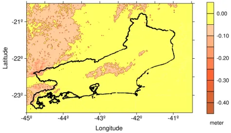
, is computed by means of Helmert’s second condensation method (Lambert 1930) from the elevation data file (Fig. 2). Finally, the

N

_STOKES

(

φ

,

λ

)

component is computed from Eq. (4) with the residual free-air anomalies (free-air anomalies minus anomalies derived from model), corrected for the topographic relief and atmospheric attraction effects.

Both Delaunay and Voronoi schemes were used to compute

N

STOKES

(

φ

,

λ

)

(10)

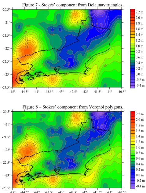
3 8 7 Figure 7 - Stokes’ component from Delaunay triangles.

Figure 8 – Stokes’ component from Voronoi polygons.

Involving almost the double of discretization cells, the Delaunay scheme

provides a more smoothed aspect in

N

STOKES

(

φ

,

λ

)

_{component than the Voronoi}

scheme, what leads to a residual difference (Voronoi minus Delaunay) as is -45° -44.5° -44° -43.5° -43° -42.5° -42° -41.5° -41° -40.5°

-23.5° -23° -22.5° -22° -21.5° -21° -20.5°

-0.4 m -0.2 m 0.0 m 0.2 m 0.4 m 0.6 m 0.8 m 1.0 m 1.2 m 1.4 m 1.6 m 1.8 m 2.0 m 2.2 m

-45° -44.5° -44° -43.5° -43° -42.5° -42° -41.5° -41° -40.5° -23.5°

-23° -22.5° -22° -21.5° -21° -20.5°

(11)

3 8 8

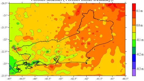
indicated in figure 9. The discrepancies range from -35 cm to 14 cm, with mean value of -2 cm and standard deviation of 4 cm.

Figure 9 – Differences between geoidal heights computed with Delaunay and Voronoi schemes (Voronoi minus Delaunay).

A comparison between the application of Delaunay and Voronoi schemes and the classical technic in geoidal heights computation was done. As the first two terms in Eq. (6) are independent of the used method to compute Stokes’ integral, because they do not depend on the way as the discretization is carried out, to examine the differences it is sufficient to consider only the term

N

_STOKES

(

φ

,

λ

)

.

Table 1 presents the statistics of those differences for the Rio de Janeiro dataset. The RMS differences indicate an almost perfect agreement (99%) between the Voronoi and Delaunay schemes. Only one point in the Voronoi scheme is outside the 99% confidence interval for the RMS difference, which the maximum difference is less than 10 cm. With the exception of the area of Corcovado peak, results are statistically the same for the two methods.

Table 1 - Differences (metres) between the classical numerical integration technique and Voronoi Delaunay.

Statistics Voronoi Delaunay

RMS difference 0.022 0.024

Minimum -0.028 -0.013 Maximum 0.080 0.085 -45° -44.5° -44° -43.5° -43° -42.5° -42° -41.5° -41° -40.5°

-23.5° -23° -22.5° -22° -21.5° -21° -20.5°

(12)

3 8 9

3.2 The Terrain Correction Computation

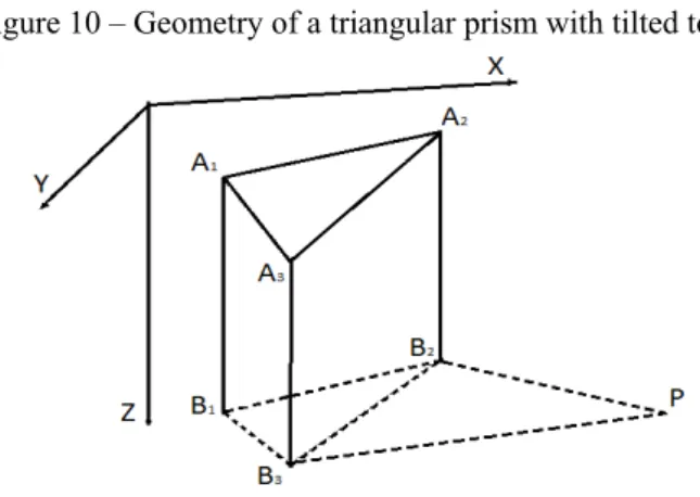
The terrain correction takes into account the attraction effect of the irregularities of the topography in the vicinity of the gravity station and is always added to the observed value. Since the terrain correction can take values larger than other corrections to gravity (Earth's tide, free-air, Bouguer) it is very important, mainly in regions of rugged topography. The gravitational attraction of a vertical triangular prism is the mathematical model used here for the terrain correction computation (WOODWARD, 1975, RUPERT, 1988). The terrain is geometrically represented by vertical prisms of triangular base (B1, B2, B3) in horizontal plane at the altitude of the gravity point (P) and tilted top (A1, A2, A3) modeling the topography (Figure 10). Vertices of the triangular base are determined according to the Delaunay structures and the density is assumed to be constant. Within a given radial distance from each gravity point, the calculation of the vertical component of attraction of the prisms is computed.

Figure 10 – Geometry of a triangular prism with tilted top.

(13)

3 9 0

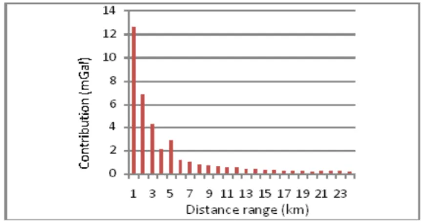
contribution, in mGal, per distance range, in km, up to 24 km from the point of maximum value of terrain correction (37.22 mGal), it is possible observe that, for distances larger than 24 km, the contribution to terrain correction tends to zero. The Figure 12 shows the map of the terrain correction in Rio de Janeiro State area, computed using Delaunay triangulation (Figure 4) and the dataset presented in Figure 3.

Figure 11 – Contribution per distance range in the terrain correction at the point of maximum value, up to 24 km from the point.

Figure 12 – Terrain correction on State of Rio de Janeiro area, with the curve of 2 mGal in highlight, as it was computed using Delaunay triangulation.

-45º -44º -43º -42º -41º

Longitude -23º

-22º -21º

Lat

it

ude

0 10 20 30 40

(14)

3 9 1

3.3 The Indirect Effect Correction

As gravity reductions deal with topographic mass displacement, the resulting indirect effect on the geoidal height must be computed (HEISKANEN & MORITZ, 1967). The Helmert's second method of condensation involves generally small indirect effects, given by (SIDERIS and SHE, 1995):

)

(

1

6

3 3 1

3 2

i P N

i i i P

EFFECT

H

s

a

G

H

G

N

=

−

+

∑

−

=

γ

ρ

γ

ρ

π

(8)

where si is the Euclidean distance from computation point P, with elevation HP, to

generic integration cells i, with elevation Hi and area ai.

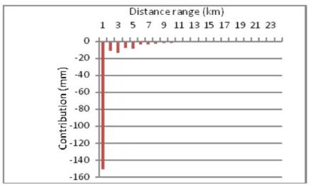
Using the same process applied to the terrain correction, with the same Delaunay scheme, dataset and scanned distance, the indirect effect for Helmert’s second method of condensation was computed. The values range between -0.424 m and 0 m. The mean value and standard deviation are, respectively, of -0.025 m and 0.032 m.

Figure 13 – Contribution per distance range in the indirect effect correction at the point of minumum value, up to 24 km from the point.

(15)

3 9 2

Figure 14 – Indirect effect for the Helmert’s second condensation method, with the curve of -0.05 meter in highlight, as it was computed using Delaunay triangulation.

3.4 THE GRADIENT OF THE HELMERT GRAVITY ANOMALY

For the solution of some geodetic problems, involving downward or upward continuation of the gravity, it is useful to know the gradient of the gravity anomaly,

∂Δg/∂H, which can be derived, assuming H and the radius vector, r, in the same direction (HEISKANEN and MORITZ, 1967, page 115, Eq. 2-217):

P

_g

R

d

l

g

R

r

g

₌

Δ

−

Δ

₋

_Δ

∂

Δ

∂

∫∫

2

3

2

σ

π

_σ , (9)

where

Δ

gP isreferred to a fixed point P on which ∂Δg/∂r is to be computed; R is the

mean radius of the earth; l is the spatial distance between the fixed point P and the variable surface element R2 dσ, expressed in terms of the angular distance ψ by

2 ψ

2 Rsin

l

=

. (10)

The Eq. (24) can be written as

P

_g

R

d

l

g

R

H

g

Δ

−

Δ

−

Δ

=

∂

Δ

∂

∫∫

2

3

2

σ

π

_σ , (11)

without error larger than 0.0006 %.

-45º -44º -43º -42º -41º

Longitude -23º

-22º -21º

La

ti

tud

e

-0.40 -0.30 -0.20 -0.10 0.00

(16)

3 9 3 Since the gravity anomaly is not known as a continuous function, a numerical integration, based on Eq. (10), may be used for computing its vertical gradient, by discretizing the earth surface in cells, that is:

(

i P

)

n

i i i

P

g

l

a

g

R

H

g

₌

₋

_Δ

₊

_Δ

₋

_Δ

∂

Δ

∂

∑

=1 3

2

1

2 π

(12)

where n is the number of cells over the integrating area around the point P, i is the order of a generic cell with area ai and mean gravity anomaly value

Δ

gi. As the

summation decreases very rapidly with increasing distance, it is sufficient to extend the numerical integration over the immediate neighborhood of the point P.

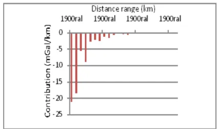
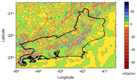
Vertical gradients of the Helmert gravity anomaly were computed for State of Rio de Janeiro area in a 1.5-arcmin grid, using Delaunay triangulation (Figure 4) and the dataset presented in Figure 3. A grid of 1.5-arcmin horizontal resolution was used to fill in the blank areas. The neighboring area was scanned up to a radial distance of 24 km. The values of the gradient vary from -68.6 mGal/km to 27.2 mGal/km.

Figure 15 – Contribution per distance range in the vertical gradient of Helmert gravity anomaly at the point of minumum value, up to 24 km from the point.

(17)

3 9 4

km, the contribution tends to zero. A map for the vertical gradient of the Helmert gravity anomaly is shown in the Figure 16.

Figure 16 – Vertical gradient of Helmert gravity anomaly with the curve of zero mGal/km in highlight, as it was computed using Delaunay triangulation.

4. CONCLUSIONS

Voronoi and Delaunay structures have been applied as alternative discretization tools to compute numerical surface integration in geodetic problems solutions, when under the integral there is a non-analytical function. Both schemes were used to computing the Stokes’ integral, while terrain correction, indirect effect and vertical gradient of the Helmert gravity anomaly were computed using Delaunay triangulation.

The main advantage of those schemes is to perform the computation without an interpolation grid, when the amount and distribution of data points are enough. Even when this condition is not satisfied, it is possible to merge data points with a grid of interpolated data, used to fill in the blank areas. In both cases, the original data are preserved. However, when merged data are used, it is important to check the consistency between the interpolated data grid and the original data. Any bias or conflict should be eliminated a priori, to avoid artificial effects on results.

Both structures, of simple and efficient geometrical constructions, are useful for the tessellation of a site in order to evaluate the geoidal undulations by means of the Stokes’ technique. The Voronoi approach uses less discretization cells than the Delaunay triangulation, nevertheless, both schemes leads to the same results, which are somewhat more efficient than the classical method.

-45º -44º -43º -42º -41º

Longitude -23º

-22º -21º

La

ti

tude

-60 -40 -20 0 20

(18)

3 9 5 Although a test with Voronoi scheme could have been done to the computation of terrain corrections, indirect effects and vertical gradients of the Helmert gravity anomaly, it was the Delaunay triangulation used here, having in sight the best fit of the triangles to rugged surfaces. For the sake of comparison, a test with Voronoi scheme could have been done.

REFERENCES

AURENHAMMER F. Voronoi diagrams: A survey of a fundamental geometric data structure. ACM Computing Surveys23(3): 345-405,1991.

AYHAN M.E. Updating and computing the geoid using two dimensional fast Hartley transform and fast T transform. Journal of Geodesy 71: 362-369,1997. DENKER H., WENZEL H.G. Local geoid determination and comparison with GPS

results. Bulletin Géodésique 61: 349-366,1987.

FORSBERG R., SIDERIS M.G. Geoid computations by the multi-band spherical FFT approach. Manuscripta Geodaetica 18: 82-90,1993.

GEMAEL C. Introdução à Geodésia Física. 1999. UFPR, Curitiba, Brazil

GOLDEN SOFTWARE Surfer Version 7 User Guide. 1999. Golden Software Inc., Golden, Colorado

GUIMARÃES G. do N., BLITZKOW D. Problema de valor de contorno da Geodésia: uma abordagem conceitual. Boletim de Ciências Geodésicas vol.17 no.4, p. 607-624, Curitiba Oct./Dec., 2011.

HAAGMANS R.R., DE MIN E., VAN GELDEREN M. Fast evaluation of convolution integrals on the sphere using 1D FFT, and a comparison with existing methods for Stokes’ integral. Manuscripta Geodaetica 18: 227-241,1993.

HEISKANEN W.H., MORITZ H. Physical Geodesy. 1967. WH Freeman & Co, San Francisco

HIRVONEN R.A. On the precision of the gravimetric determination of the geoid. Transactions - American Geophysical Union 3 (1): 1-8, 1956.

JIANG Z., DUQUENNE H. On fast integration in geoid determination. Journal of Geodesy 71: 59-69, 1997.

KUROISHI Y. An improved gravimetric geoid for Japan, JGEOID98, and relationships to marine gravity data. Journal of Geodesy 74 (11-12): 745-765, 2001.

LAMBERT W.D. The reduction of observed values of gravity to sea level. Bulletin Géodésique 26: 107-181, 1930.

LEHMANN R. Fast space-domain evaluation of geodetic surface integrals. Journal of Geodesy 71: 533-540, 1997.

LI J., SIDERIS M.G. The fast Hartley transform and its application in physical geodesy. Manuscripta Geodaetica 17: 381-387, 1992.

MORITZ H. Geodetic Reference System 1980, Bulletin Géodésique 58 (3): 388-398, 1984.

(19)

3 9 6

geopotential and sea surface topography harmonic coefficient models. 1991. Rep 410, Department of Geodetic Science and Surveying, The Ohio State Univ, Columbus

RAPP R.H., BASÍC T. Ocean-wide gravity anomalies from GEOS-3, Seasat and Geosat altimeter data. Geophysical Research Letters 19(19): 1979-1982, 1992. RUPERT J. A gravitational terrain correction program for IBM compatible

personal computers. 1988.Vol. 2.21, Geological Survey of Canada, GSC, Open File 1834

SANTOS N.P., ESCOBAR I.P. Gravimetric geoid determination in the municipality of Rio de Janeiro and nearby region. Brazilian Journal of Geophysics 18 (1): 49-62, 2000.

SANTOS N.P. and ESCOBAR I.P.,2010. Use of EGM08 model and Shuttle Radar Topography Mission data for geoid computation in the State of Rio de Janeiro, Brazil: a case of study with Voronoi/Delaunay discretizations. Studia Geophysica et Geodaetica, 54: 239-255

SIDERIS M.G., TZIAVOS I.N. FFT-evaluation and applications of gravity-field convolution integrals with mean and point data. Bulletin Géodésique62: 521-540, 1988.

SIDERIS M.G., SHE B.B. A new high-resolution geoid for Canada and part of the U. S. by the 1D-FFT method. Bulletin Géodésique 69: 92-108, 1995.

SIDERIS M.G. Fourier geoid determination with irregular data. Journal of Geodesy 70: 2-12, 1995.

STOKES G.G.) On the variation of gravity on the surface of the Earth. In: Mathematical and Physical Papers, Vol. II, New York, pp 131-171 (from the

Transactions of the Cambridge Philosophical Society, Vol. VIII, pp 672-695) , 1849.

STRANG VAN HEES G.L. Precision of the geoid, computed from terrestrial gravity measurements. Manuscripta Geodaetica 11: 86-98, 1986.

TSAI V.J.D. (1993) Fast topological construction of Delaunay triangulations and Voronoi diagrams. Computers & Geosciences 19(10): 1463-1474

VINCENTY T. Direct and inverse solutions of geodesics on the ellipsoid with application of nested equations. Survey Review, XXII(176),88–93, 1975. WOODWARD D.J. The gravitational attraction of vertical triangular prisms,

Geophysical Prospecting, 23(3): 526-532, 1975, 1975.