Genome Markers
Gustavo de los Campos*, Yann C. Klimentidis, Ana I. Vazquez, David B. Allison
Section on Statistical Genetics, Department of Biostatistics, University of Alabama at Birmingham, Birmingham, Alabama, United States of America
Abstract
Genetic factors are believed to account for 25% of the interindividual differences in Years of Life (YL) among humans. However, the genetic loci that have thus far been found to be associated with YL explain a very small proportion of the expected genetic variation in this trait, perhaps reflecting the complexity of the trait and the limitations of traditional association studies when applied to traits affected by a large number of small-effect genes. Using data from the Framingham Heart Study and statistical methods borrowed largely from the field of animal genetics (whole-genome prediction, WGP), we developed a WGP model for the study of YL and evaluated the extent to which thousands of genetic variants across the genome examined simultaneously can be used to predict interindividual differences in YL. We find that a sizable proportion of differences in YL—which were unexplained by age at entry, sex, smoking and BMI—can be accounted for and predicted using WGP methods. The contribution of genomic information to prediction accuracy was even higher than that of smoking and body mass index (BMI) combined; two predictors that are considered among the most important life-shortening factors. We evaluated the impacts of familial relationships and population structure (as described by the first two marker-derived principal components) and concluded that in our dataset population structure explained partially, but not fully the gains in prediction accuracy obtained with WGP. Further inspection of prediction accuracies by age at death indicated that most of the gains in predictive ability achieved with WGP were due to the increased accuracy of prediction of early mortality, perhaps reflecting the ability of WGP to capture differences in genetic risk to deadly diseases such as cancer, which are most often responsible for early mortality in our sample.
Citation:de los Campos G, Klimentidis YC, Vazquez AI, Allison DB (2012) Prediction of Expected Years of Life Using Whole-Genome Markers. PLoS ONE 7(7): e40964. doi:10.1371/journal.pone.0040964
Editor:Nicholas John Timpson, University of Bristol, United Kingdom
ReceivedSeptember 8, 2011;AcceptedJune 15, 2012;PublishedJuly 25, 2012
Copyright:ß2012 de los Campos et al. This is an open-access article distributed under the terms of the Creative Commons Attribution License, which permits unrestricted use, distribution, and reproduction in any medium, provided the original author and source are credited.
Funding:This project had funding from National Institutes of Health grants P30CA13148, P30DK056336, R01GM077490, R01DK076771, T32HL105346 and KRAFT-grant ‘‘University of Alabama at Birmingham doctorate Training Program in Obesity and Nutrition Research.’’ The funders had no role in study design, data collection and analysis, decision to publish, or preparation of the manuscript.
Competing Interests:The authors have declared that no competing interests exist. * E-mail: [email protected]
Introduction
Agricultural and biomedical research has shown through controlled experiments and familial studies that many complex traits are highly heritable, suggesting that in principle, such traits could be predicted early in life from knowledge of individuals’ genotypes. Human longevity is not an exception: empirical evidence from twin and familial studies indicate that approxi-mately 25% of inter-individual differences in human lifespan can be attributed to genetic factors [1–3].
Research with model organisms offers several examples of genetic polymorphisms having a sizable effect on lifespan [4]. However, although genome-wide association studies (GWAS) and linkage scans in humans have uncovered several regions signifi-cantly associated with longevity and aging traits [5–9], only a few of these associations have been consistently confirmed, and our ability to predict inter-individual differences in expected Years of Life (YL) remains limited [7].
Several diseases (e.g., cancer, cardiovascular disease) and biological events (e.g., stroke, heart failure) can lead to death, and the genetic architecture (i.e., the set of genes having an effect on the trait and the ways they interact) of each of these mortality-related traits is expected to be disorder-specific. Therefore, the
genetic architecture of YL is likely to include a large number, perhaps thousands, of possibly interacting genes.
Recent articles [10,11] have suggested that the limited advances in our ability to predict complex human traits and diseases using genomic information may partially reflect the limitations of traditional GWAS to detect significant associations with complex genetic architectures. These authors have suggested that Whole Genome Prediction (WGP) may be better suited than traditional GWAS to the prediction of complex traits.
Whole genome prediction exploits multi-locus linkage-disequilibrium (LD) between quantitative trait loci (QTL) and genome-wide markers (e.g., SNPs) to predict inter-individual differences in a quantitative trait that are attributable to genetic factors. Unlike traditional association studies, in which the association between markers and phenotypes is tested one marker at a time, WGP uses all available markers to regress phenotype onto genomic information. This methodology was first proposed in the field of animal breeding by Meuwissen Hayes and Goddard in 2001 [12]. Since then, several simulation [12,13] and empirical studies have demonstrated its predictive power with plant [14,15] and animal [16–19] data.
and, more importantly, that regression using WGP methods can improve the prediction of yet-to-be observed human phenotypes [20]. A next logical question is whether these findings apply to traits of greater medical or practical importance. Here, we: (a) extend WGP methods, which were originally developed for continuous un-censored outcomes, to accommodate censoring, a feature commonly encountered in applications with human data, (b) developed a WGP model for YL and (c) quantified the ability of this model to account for and to predict inter-individual differences in human YL that are not accounted for by major factors such as sex, Body Mass Index (BMI, kg/m2) and smoking.
Materials and Methods
Model
Many outcomes in human-health studies are either binary (e.g., presence/absence of diseases) or are subject to censoring (i.e., bounds of the outcome are known, but the exact value of outcome remains unknown). And it is well established that ignoring censoring yields biased estimates [21]. The linear models commonly used for WGP can be easily extended to accommodate binary or censored outcomes. Here, we present an extension that accommodates censoring. Similar ideas can be used to model binary outcomes as well [22].
In our WGP models, we describe YL (yi,i = 1,…,n) as the sum
of individual-specific means (mi) which, as we explain below, will be a function of genetic and non-genetic factors, and of a model residual (ei) which is assumed to be a normal random variable with
mean zero and variances2; thereforey
i~mizei. For individuals
with known YL, we observeyi; for individuals with censoring at
age equal toti, the observed event isyiwti. In our WGP model, expected YL (mi) was described using a linear regression,
mi~mzXJ
j~1xijcjz XL
l~1zilbl, ð1Þ which had three components:m, an effect common to all subjects; PJ
j~1xijcj, a regression component accounting for the effects of
non genetic covariates (sex, smoking and BMI covariates in our application); andPL
l~1zilbl, a regression on SNP genotypeszij
where zij[f0,1,2g counts the number of copies of the least frequent allele at thejthSNP. By combining (1) with the normal assumptions described above, we derived the likelihood function for censored and un-censored individuals (see Methods S1 for further details).
The Bayesian model is completed by assigning a prior density to the collection of model unknownsfm,c,b,s2g. Here, we structure the prior density using a modified version of the Bayesian LASSO (BL) [23]. This model has been effectively used for WGP in plants [14,15,24], animals [14,18,19,25] and humans [20]. We extend this model to accommodate censoring as well as effects other than those of markers. In our model, we assigned independent vague prior densities to the intercept (m) and to the effects of sex, smoking and BMI (c). This treatment yields estimates of the effects of these non-genetic factors that are similar to those obtained with likelihood-based methods. For the remaining unknowns we adopt the prior-specification of the BL of Park and Casella [23] (see Methods S1 for further details). The joint prior-density (see expression 2 in the Methods S1) is indexed by a set of four hyper-parameters, including the prior degree of freedom and scale assigned to the residual variance (denoted asdfandS, respectively), and the rate and shape parameters (dentoed as d and s, respectively) assigned to the regularization parameter of the BL. A discussion of how these can be chosen is given in Perez et al.
[26]. Here, following those guidelines, we set H~df~5,S~170,d~1|10{4,s~2
. Given the characteris-tics of our data (sample size, number of markers and allele frequencies and observed variability on YL), these values provide priors with small influences on predictions.
Implementation
Models were fitted using a modified version of the BLR package [27] of R [28] which handles censoring (right, left and interval) according to the model described above. In addition to BLR, R-packages bayesm [29], splines [28] and SuppDists [30] were used to implement the sampler.
Data
(N = 5,117) were from the original (N = 1,493) and offspring (N = 3,624) cohorts of the Framingham Heart Study. Data and material distributions from this study are made in accordance with the individual consent history of each participant (see http://www. framinghamheartstudy.org/research/consentfms.html for further details about consent forms). And the current study has been approved by the Internal Review Board of University of Alabama at Birmingham (IRB Protocol Number: X090720002). The criteria for inclusion in the study included being 18 years or older at time of recruitment, having survival information as of 2007, and having complete information for covariates (sex, smoking and BMI).
Average age at entry was 37 with a standard deviation (SD) of 9.0 years. Of the participants, two thirds (N = 3,390) were censored (i.e., at the time at which survival records were defined, these individuals were still alive), 55% were female, and 36% never smoked. Mean BMI at first exam was 25.0 with a SD of 4.1 kg/ m2. Subjects were genotyped using the Affymetrix GeneChip Human Mapping 500K Array Set. For details on the genotyping method, please refer to Framingham SHARe at the NCBI dbGaP website (http://www.ncbi.nlm.nih.gov/projects/gap/cgi-bin/ study.cgi?study_id = phs000007.v3.p2). Other editing and geno-typing quality control and imputation procedures were as described in Makowsky et al. [20].
Primary Data Analysis
Using the specification of equation (3) we generated a sequence of nested models by changing the predictors included in the right-hand side of the linear predictor (mi). Our baseline model (denoted as MA-0) includes an intercept, sex, and age at entry; the latter
modeled nonparametrically using a 4-df natural spline [31] with interior and boundary knots chosen using the default specifications of the natural spline (ns) function of the spline package of R [28]; with 4-df, interior knots were placed at the 25th, 50th and 75th sample percentiles of the predictor variables. We extended this model by adding smoking and BMI (also modeled nonparame-terically using a 4-df natural spline [31]) this model is denoted as MB-0. Subsequently, models MA-0and MB-0were then extended
by adding subsets of evenly spaced SNPs, from 2.5K (K = thou-sand) to 80K; these models were denoted as M(.)-2.5K, M(.)-5K,
M(.)-10K, M(.)-20K, M(.)-40Kand M(.)-80K, where (.) was either A or B.
Models were first fitted to the entire dataset to obtain parameter estimates (estimated posterior means of effects and of variance parameters) and to evaluate the goodness of fit and the Deviance Information Criterion [32]. Subsequently, the prediction accuracy of each of the models was assessed using a 10-fold cross-validation (CV). Prediction accuracy was evaluated using two different metrics: a CV R-squared (R2
CV) and the area under Longitudinal
R2
CV measures the proportion of inter-individual differences in
years of life that can be accounted by CV-predictions, this was
calculated as R2
CV~1{
X
i[U
yi{mm^i,M:
2
X
i[U
yi{^mmi,MA{0
2 where: yi denotes
observed YL of the ith individual, mm^i,M
A{0 is a 10-fold
CV-prediction of YL derived from model M: and mm^i,MA{0 is the
estimated average YL, derived from a model that only included an intercept and the effect of age at entry, which is taken here as our baseline model. This statistic can be evaluated only with subjects that have already died; therefore, in the 10-fold CV, the summation in the formula for R2
CV uses only data from subjects
with an observed age at death. Un-censored subjects do not constitute a random sample of individuals and this may induce bias in our estimate of R-squared. Because of this, we consider a second measure of prediction performance based on longitudinal AUCs [33]. To this end we defined a sequence of thresholds (t= 60, 65, 70, 75, 80, 85, 90, 95 YL) and for each of these thresholds we generated survival indicator variables di,60,di,65,…,di,95 where:di,t~1if individualihad YL,t;di,t~0 if individual i was still alive at time t, and un-determined if individualihad an age at censoring smaller thant. The number of individuals for which di,t was determined (i.e., those that had
known YL or age at censoring greater thant) were 4495, 3836, 3262, 2773, 2366, 2102, 1889 and 1762 for t~65,…, t~95, respectively. Using these survival indicator variables and CV predictions of YL (^mmi,M
:) derived from the models above described we computed the AUC(t) for every threshold using the R-package pROC [34].
Evaluation of the effects of population structure and familial relationships on prediction accuracy
The distribution of genotypes, their allele frequency, levels of LD, etc., can be affected by factors such as population structure, admixture or familial relationships. Therefore, a certain propor-tion of the predicpropor-tion accuracy of WGP could be attributed to those factors. To further explore this, a series of additional analysis were carried out. First, in order to account for population structure, we extended the model including age, sex, smoking and BMI as predictors (MB-0) by adding the effects of the first two
principal components (PCs) derived from the same set of 80K SNPs used in M(.)-80K. Second, to quantify the relative
importance of familial relationships on prediction accuracy we carried out two additional analyses: (a) we extended MB-0 by
adding an effect representing a regression on the pedigree. This was done using the standards of the additive infinitesimal model of quantitative genetics [35], and this model is denoted as MB-PED.
And (b) we fitted models MA-0K, MB-0Kand MB-80K in a 10fold
CV where entire families, as opposed to individuals, were assigned to folds; therefore, in this CV predictions are derived from nominally-unrelated individuals.
Results
Full data analysis
Using MB-0, we estimated an average (6 posterior SD)
difference in YL between females and males of 3.1 (60.42) years and between smokers and nonsmokers of 24.1 (60.44) years. Using estimates from MB-0, we computed the expected YL of
a nonsmoking 35-year-old by sex and BMI; the results are displayed in (Figure S1). Expected YL was greatest within the range BMI[ [20,25]; extreme BMI values, lower than 20 or
higher than 25, were associated with a decrease in YL. Using MB-0
we estimate an expected decrease in YL of 0.43 year per extra unit of BMI in the rangeBMI[[25,40]. Overall, these patterns are in agreement with what has been reported previously for the effect of sex [36–38], smoking [36,39] and BMI [21,36] on YL.
Table 1 shows estimates of residual variance and DIC by model. The intercept-only model (not included in Table 1) yielded an estimate of variance of YL of 135, and the estimated residual variance of MA-0 was 104.1; therefore, approximately 23%,
computed as 100|ð1{(104:1=135)Þ, of observed variability in YL in our dataset can be explained by differences in age at entry and sex. Model MB-0 yielded an estimate of residual variance of
98.7, indicating that BMI and smoking accounted for about 5% of inter-individual differences in YL that were not accounted for by age at entry and sex; this was computed as100|ð1{98:7=104:1Þ. Adding SNPs to MA-0or MB-0resulted in a marked increase in
goodness of fit, and this is reflected in a substantial reduction in the estimated residual variance (Table 1). For instance, MB-80Kyielded
an estimate of the residual variance that was 65% smaller than that of the MB-0K, computed as100|ð1{34:4=98:7Þ.
Due to the curse of dimensionality [40], the increase in goodness of fit achieved by adding SNPs to the model may reflect genetic variability captured by SNPs, over-fitting, or a combina-tion of both. However, DIC, a model comparison criterion that balances goodness of fit and model complexity, decreased monotonically with the number of SNPs, suggesting that information is being added as marker density increases.
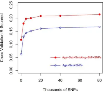
Evaluation of prediction accuracy in cross validation Figure 1 shows estimatedR2
CVversus marker density (from 0 to
80K) by model. TheR2
CV of a model including age at entry and
sex, R2
CVðMA{0Þ, was approximately 6%. The addition of smoking and BMI resulted in a doubling of R2
CV, from
R2
CVðMB{0Þ~6% to R2CVðMB{0Þ~12%; as expected, the addition of smoking and BMI increased prediction accuracy by a sizable amount. Prediction accuracy increased monotonically with the number of markers both in models with and without BMI and smoking covariates. These results confirm that markers are capturing information about expected YL that cannot be predicted using major factors such as age at entry, sex, smoking and BMI. Using 80K markers, we were able to increaseR2
CV from 6% to
11% for the model without smoking and BMI (MA-(.)) and from
12% to 21% for the model including smoking and BMI (MB-(.)).
(Table S1) showsR2
CVfor models MA-0, MB-0and MB-80Kby fold
of the CV. The variability inR2
CV across folds reflects uncertainty
about our estimates due to sampling of training and testing datasets. Although we observed an overall superiority of MB-0over
MA-0 this superiority did not occur in every fold of the CV.
However, MB-80Koutperformed models without SNP information
(MA-0and MB-0) consistently across folds indicating that SNPs are
capturing important and consistent patterns of variability in human lifespan.
The above results indicate that markers can explain a sizable proportion of inter-individual differences in YL that are not accounted for by age at entry, sex, smoking and BMI. To obtain further insights into the source of this improvement in prediction accuracy, we present in Figure 2 the average absolute value of the CV prediction error (from the 10-fold CV) and its SE by range of YL for models MB-0Kand MB-80K. As expected, for both models,
the absolute value prediction error was lowest for people dying around median age (80 YL) and increased for people dying early or late in life. Predictions derived from model MB-80Kwere much
people dying early in life; however, the prediction accuracy of the model with markers was slightly higher than that of MB-80Kfor
subjects dying at intermediate ages. This suggests that the overall higher predictive ability of MB-80Kis due mostly to improvements
in prediction of early mortality.
Figure 3 shows the AUC (vertical axis) for models MA-0, MB-0,
and MB-80Kfor each of the 8 thresholds (horizontal axis). Adding
BMI and smoking information to a model that included sex and age (MB-0vs MA-0) resulted in an increase in AUC(t) of roughly 5– 7%. When 80 thousand SNPs (MB-80K) were added to a model
that included age, sex, smoking and BMI as covariates we observed a substantial increase in classification performance for prediction of early stage survival status (relative to MB-0, MB-80K
yielded an increase in AUC(60) of 18%), a more modest increase in AUC(t) for survival status at ages 65–90 (MB-80Koutperformed MB-0by about 14% for AUC(65) and by 7–10% for AUC(70)–
AUC(90)), and no change in AUC(95). These results are consistent with those observed withR2
CV in that they indicate that genomic
information can increase the prediction accuracy of lifespan, mostly due to an increase in the prediction of early mortality. Table S1 shows estimates of AUC(t) for models MA-0, MB-0and MB-80Kby fold of the CV. Similar to what we observed forR2CV,
although we found an overall superiority in the classification performance of MB-0relative to that of MA-0such superiority was
not consistently observed in every fold. However, for early and intermediate survival status (t#85) model M
B-80Khad a
classifica-tion performance that was consistently higher than that of models without genetic information (MA-0and MB-0). For late mortality
(t.85) such superiority was not consistently observed across folds.
Effects of population structure The estimated R2
CV of model MB-GWPC was 15.77%, this is
roughly half the way from theR2
CV of model MB-0(11.45%) and
Table 1.Estimated posterior mean of residual variance and Deviance Information Criterion (DIC, ‘smaller is better’) by number of SNPs (rows) and nongenetic covariates (columns) included in the model.
Residual Variance* Deviance Information Criterion (DIC)
Thousands of SNPs in the
Model Age+Sex Age+Sex+BMI+Smoking Age+Sex Age+Sex+BMI+Smoking
0 104.1 98.7 14,744 14,625
2.5 79.7 75.5 14,268 14,158
5.0 68.3 64.1 14,130 14,007
10.0 57.1 554.5 13,951 13,845
20.0 48.1 46.2 13,772 13,673
40.0 40.3 39.6 13,540 13,479
80.0 34.6 34.4 13,337 13,289
*: Posterior mean of the residual variance, the estimate of this parameter can be regarded as a proxy of goodness of fit to the data used to train the model. doi:10.1371/journal.pone.0040964.t001
Figure 1. Cross-validation R-squared (R2
CV) by number of markers and model.Circles represent theR2
CVobtained in a 10-fold CV.
doi:10.1371/journal.pone.0040964.g001
Figure 2. Absolute value CV prediction error versus range of YL.Circles represent the average absolute value prediction error for each group of YL (YL#65, 65,YL#70,..,YL.95); and vertical bars represent the 95% confidence interval defined by the average absolute value prediction error61.966SE.
that of model MB-80K(21.40%). Results for AUC showed similar
patterns. This indicates that a sizable proportion of inter-individual differences in YL could be attributed to genetic differences associated to population structure. On the other hand, the fact that theR2
CVof model MB-80Kwas 37% higher than that
of model MB-GWPC suggests that genetic factors beyond those
associated with population structure account for a sizable proportion of inter-individual differences in YL.
Effects of familial relationships
Model MB-PED, which including age at entry, sex, BMI,
smoking and pedigree information showed clear signs of over-fitting (the posterior mean of the residual variance was 11.1, compared to 34.4 for model MB-80K) and, consequently, had a
very poor predictive performance; even worse than our baseline model (MA-0). This is most likely to occur because of two reasons.
First, the pedigree is very sparse, with 37% of nominally un-related individuals and most of the remaining individuals coming from relatively small nuclear families (74% of individuals were in families with 3 or less members). Additionally, in the great majority of nuclear families the offspring have censored YL. Therefore, in this dataset the amount of familial information available for prediction is very limited. To further illustrate this, we counted for every subject in the 10-fold CV where individuals were randomly assigned to folds the number of close-relatives (father, mother, offspring or full-sib) which were used for prediction (i.e., those which were assigned to a different fold). We found that in our CV 41.6 of the observations were predicted without having any direct relative in the training dataset (i.e. in other folds) and 70.75 were predicted without having any un-censored direct relative available for training. Only 10% of individuals had 3 or more direct relatives in the training datasets, and no-one had 3 or more direct relative with observed YL assigned to a different fold.
Our second approach to quantify the relative importance of family relationships on prediction accuracy consisted on fitting models MA-0, MB-0 and MB-80K in a10-fold CV where entire
families, as opposed to individuals, were assigned to folds. Such setting guarantees that no-direct relatives are used for prediction. TheR2
CV obtained in this new CV were very similar (R2CV were
11.9% and 22.3% for MB-0and MB-80K, respectively) to the ones
we obtained when subjects, as opposed to entire families, were assigned to folds (here,R2
CVwere 11.9% and 22.3% for MB-0and
MB-0, respectively). Combining all these results we conclude that in
our analysis familiar relationships were not a major factor explaining the prediction accuracy obtained with WGP.
Prediction accuracy and causes of mortality
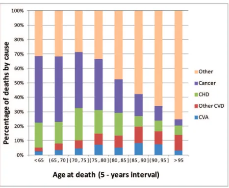
Our results suggest that genomic information can enhance prediction of lifespan, mostly by improving prediction of early mortality. This can be due to several factors, one of which may be that SNPs are capturing genetic risk to certain diseases that are most responsible for early mortality. Figure 4 presents the distribution of death by cause and range of age at death in the Framingham sample. Cancer was the leading cause of death for people dying early in life, and the relative importance of cancer as a cause of death declined with increasing YL. On the other hand, the relative importance of other causes of death was much higher for people dying at older ages.
Discussion
Familial studies suggest that roughly 25% of the inter-individual differences in YL can be attributed to genetic factors [7]. Although linkage and association studies have reported several variants associated with human lifespan and aging-related traits [6,8,9,41], the individual effects of these variants is usually small and our ability to use genetic information to predict human lifespan remains very limited. Recent studies [10,11,20] suggest that WGP is effective at predicting complex traits. Here, we developed a WGP model for the prediction of YL and evaluated its predictive power using data from the Framingham longitudinal study.
When genetic markers were added to a model accounting for age at entry, sex, smoking, and BMI, the increase inR2
CVobtained
by adding 80K SNPs (,9–10% of inter-individual differences in YL) was greater than the increase obtained by adding smoking and BMI (,6% of inter-individual differences in YL), indicating that genetic markers are making a relatively important contribution to predictive ability. Similar results were obtained when prediction accuracy was evaluated using longitudinal AUC’s.
As anticipated, our results suggest that the genetic basis of YL involves a large number of variants. The observation that DIC and prediction accuracy improved with marker density suggests that a large number of markers spread across the genome are needed to account for differences at QTLs affecting YL, and this is consistent with what one would expect for a trait that conforms to an ‘‘infinitesimal’’ model [42,43]. This pattern is also consistent with empirical evidence obtained for traits that conform to the infinitesimal model, such as human height [20] or production traits in dairy cattle [19].
Our results are also consistent with those of Yashin et al. [44] who, using a subset of the dataset used here (1,173 individuals of the original cohort), found that a sizable proportion of inter-individual differences in YL (20% in the training dataset) can be explained by the joint influence of 168 small-effect genetic variants which were pre-selected usingp-valuesderived from single-marker regressions. Although the study by Yashin et al. [44] and the one presented here both suggest that a large number of variants is needed to account for interindividual differences in YL, the two studies differ in many respects: (a) our study uses a larger sample size (N = 5,117, versus N = 1,173) and incorporates both
sored and censored observations, (b) unlike the Yashin study, where markers were pre-selected using statistics derived from single marker regression, here we used a much larger number of markers (up to 80K), spread along the whole genome, (c) although the two studies used an additive linear score to predict YL, the two scores are different. In the Yashin study the score consist of a sum of so-called ‘‘longevity alleles’’, while in our study the predictive score is a weighted sum of allele dosage, with weights given by estimates of marker effects, (d) in some of our models we account for the effects of BMI and smoking, while these covariates were not accounted for in the Yashin study. Finally (d) in our study we focused on prediction accuracy of yet-to be observed outcomes, while the study by Yashin et al. reports the proportion of interindividual differences in YL that could be accounted for in the same dataset that was used to derive the predictive score. Nevertheless, despite the differences in the datasets and methods used, both studies provide consistent evidence that an important proportion of differences in YL can be predicted using genomic information and that capturing those patterns requires considering a large number of small-effects variants.
In addition to demonstrating that a sizable proportion differences in YL can be predicted using genomic information, we found that most of the gains in prediction accuracy obtained with use of genetic information came from increased accuracy of prediction of early mortality. Further examination of the distribution of causes of death by age at death reveled that cancer was the leading cause of death for people dying early in life. Therefore, a possible explanation of our results is that the ability of our WGP to capture cancer risk (indirectly through YL) was higher than for other death-related disorders. Further studies, using disorder-specific responses (e.g., presence/absence or onset of cancer) and case-control datasets will be needed to confirm this conjecture.
The Framingham dataset has a familial design and exhibits some level of population structure, much of which can be
described through PCA of genome-wide SNPs. Whole-Genome Prediction exploits multi-locus LD between markers and QTL. These patterns of LD are likely to change across sub-groups in the population and because of this, models fitted using WGP cannot be regarded as ‘universal equations’. The validity across sub-groups of the patterns captured by a WGP model will depend on the extent to which genetic features (e.g., stratification) present in training samples are also present in those used for validation.
Including the first two marker-derived PCs increased prediction accuracy markedly, indicating that YL covariates with ancestry, as described by the first 2 PCs. However, the level of prediction accuracy attained by models using the first two marker-derived PCs was substantially lower than that of the model using 80K genome-wide SNPs, suggesting that the genetic factors affecting YL cannot be fully described by features such as population structure. The effects of familial relationships on the prediction accuracy of WGP are well established [13,20]. However, in our study, the pedigree is relatively sparse and when families with more than one subject exist the offspring are highly likely to be censored; therefore, familiar relationships are not very informative to begin with, explaining why in this study familial relationships did not show a strong effect on the prediction accuracy of WGP.
Supporting Information
Methods S1 Describes the Bayesian model used.
(DOCX)
Figure S1 Estimated expected years of life versus Body
Mass Index (BMI) by sex (estimates derived from a model which included sex, age at entry, smoking and BMI as predictors).
(TIFF)
Figure 4. Proportion of deaths by cause, and range of age at death.Causes included cancer, coronary heart disease (CHD), cardio-vascular accident (CVA), other cardio-vascular diseases (Other CVD) and other causes.
Table S1 Cross-validation R-squared and Area Under Longitudinal Receiver Operating Characteristic Curves by model and fold of a 10-fold cross-validation.
(DOC)
Acknowledgments
The authors would like to thank the participants and organizers of the Framingham Heart Study, Sir David Cox and Drs. Henry Robertson and Emily Dhurandhar for comments and suggestions provided on an early
draft of the manuscript and Vinodh Srinivasasainagendra for assistance in downloading the dataset. Insightful suggestions made by the associate editor and two anonymous reviewers are gratefully acknowledged.
Author Contributions
Conceived and designed the experiments: GDLC YCK AIV DBA. Analyzed the data: GDLC AIV. Wrote the paper: GDLC YCK AIV DBA. Designed the software used in the analysis: GDLC.
References
1. Hjelmborg JB, Iachine I, Skytthe A, Vaupel JW, McGue M, et al. (2006) Genetic influence on human lifespan and longevity. Human genetics 119: 312–321. 2. Herskind AM, McGue M, Holm NV, S\o¨rensen TI., Harvald B, et al. (1996)
The heritability of human longevity: a population-based study of 2872 Danish twin pairs born 1870–1900. Human Genetics 97: 319–323.
3. Iachine IA, Holm NV, Harris JR, Begun AZ, Iachina MK, et al. (1998) How heritable is individual susceptibility to death? The results of an analysis of survival data on Danish, Swedish and Finnish twins. Twin research 1: 196–205. 4. Braeckman BP, Vanfleteren JR (2007) Genetic control of longevity in C. elegans. Experimental Gerontology 42: 90–98. doi:doi: DOI: 10.1016/j. exger.2006.04.010
5. Puca AA, Daly MJ, Brewster SJ, Matise TC, Barrett J, et al. (2001) A genome-wide scan for linkage to human exceptional longevity identifies a locus on chromosome 4. Proceedings of the National Academy of Sciences of the United States of America 98: 10505–10508.
6. Newman AB, Walter S, Lunetta KL, Garcia ME, Slagboom PE, et al. (2010) A meta-analysis of four genome-wide association studies of survival to age 90 years or older: the Cohorts for Heart and Aging Research in Genomic Epidemiology Consortium. The Journals of Gerontology Series A: Biological Sciences and Medical Sciences 65: 478–487.
7. Christensen K, Johnson TE, Vaupel JW (2006) The quest for genetic determinants of human longevity: challenges and insights. Nat Rev Genet 7: 436–448. doi:10.1038/nrg1871
8. Sebastiani P, Solovieff N, Puca A, Hartley SW, Melista E, et al. (2010) Genetic signatures of exceptional longevity in humans. Science.
9. Lunetta K, D’Agostino R, Karasik D, Benjamin E, Guo CY, et al. (2007) Genetic correlates of longevity and selected age-related phenotypes: a genome-wide association study in the Framingham Study. BMC medical genetics 8: S13. 10. de los Campos G, Gianola D, Allison DB (2010) Predicting genetic predisposition in humans: the promise of whole-genome markers. Nat Rev Genet 11: 880–886. doi:10.1038/nrg2898
11. Yang J, Benyamin B, McEvoy BP, Gordon S, Henders AK, et al. (2010) Common SNPs explain a large proportion of the heritability for human height. Nature genetics 42: 565–569.
12. Meuwissen TH, Hayes BJ, Goddard ME (2001) Prediction of total genetic value using genome-wide dense marker maps. Genetics 157: 1819–1829.
13. Habier D, Fernando RL, Dekkers JCM (2007) The impact of genetic relationship information on genome-assisted breeding values. Genetics 177: 2389–2397.
14. de los Campos G, Naya H, Gianola D, Crossa J, Legarra A, et al. (2009) Predicting quantitative traits with regression models for dense molecular markers and pedigree. Genetics 182: 375–385.
15. Crossa J, de los Campos G, Perez P, Gianola D, Burguen˜o J, et al. (2010) Prediction of genetic values of quantitative traits in plant breeding using pedigree and molecular markers. Genetics 186: 713–724.
16. VanRaden PM, Van Tassell CP, Wiggans GR, Sonstegard TS, Schnabel RD, et al. (2009) Invited review: reliability of genomic predictions for North American Holstein bulls. Journal of Dairy Science 92: 16–24.
17. Hayes BJ, Bowman PJ, Chamberlain AJ, Goddard ME (2009) Invited review: Genomic selection in dairy cattle: Progress and challenges. Journal of Dairy Science 92: 433–443.
18. Weigel KA, de Los Campos G, Vazquez AI, Rosa GJM, Gianola D, et al. (2010) Accuracy of direct genomic values derived from imputed single nucleotide polymorphism genotypes in Jersey cattle. J Dairy Sci 93: 5423–5435. doi:10.3168/jds.2010-3149
19. Vazquez AI, Rosa GJM, Weigel KA, de Los Campos G, Gianola D, et al. (2010) Predictive ability of subsets of single nucleotide polymorphisms with and without parent average in US Holsteins. Journal of dairy science 93: 5942–5949. 20. Makowsky R, Pajewski NM, Klimentidis YC, Vazquez AI, Duarte CW, et al.
(2011) Beyond Missing Heritability: Prediction of Complex Traits. PLoS Genet 7: e1002051.
21. Fontaine KR, Redden DT, Wang C, Westfall AO, Allison DB (2003) Years of life lost due to obesity. JAMA: The Journal of the American Medical Association 289: 187–193.
22. Lee SH, Wray NR, Goddard ME, Visscher PM (2011) Estimating missing heritability for disease from genome-wide association studies. The American Journal of Human Genetics.
23. Park T, Casella G (2008) The bayesian lasso. Journal of the American Statistical Association 103: 681–686.
24. de los Campos G, Gianola D, Rosa GJM, Weigel KA, Crossa J (2010) Semi-parametric genomic-enabled prediction of genetic values using reproducing kernel Hilbert spaces methods. Genetics Research 92: 295–308.
25. Weigel KA, De Los Campos G, Gonza´lez-Recio O, Naya H, Wu XL, et al. (2009) Predictive ability of direct genomic values for lifetime net merit of Holstein sires using selected subsets of single nucleotide polymorphism markers. Journal of dairy science 92: 5248–5257.
26. Pe´rez P, de los Campos G, Crossa J, Gianola D (2010) Genomic-Enabled Prediction Based on Molecular Markers and Pedigree Using the Bayesian Linear Regression Package in R. The Plant Genome Journal 3: 106–116. doi:10.3835/ plantgenome2010.04.0005
27. de los Campos G, Pe´rez P (2010) BLR: Bayesian linear regression. R package version 1.2. R-project, available at: http://cran.r-project.org/web/packages/ BLR/index.html. Accessed 2012 June 28th.
28. R Development Core Team (2010) R: A language and environment for statistical computing. R Foundation for Statistical Computing, Vienna, Austria. R Foundation for Statistical Computing. R-project, available at: http://www. R-project.org. Accessed 2012 June 28th
.
29. Rossi P, McCulloch R (2010) bayesm: Bayesian inference for marketing/micro-econometrics. R package version: 2–2.
30. Wheeler B (2008) SuppDists: Supplementary distributions. R package version: 1–1.
31. Hastie TJ, Tibshirani RJ (1990) Generalized additive models. Chapman & Hall/ CRC.
32. Spiegelhalter DJ, Best NG, Carlin BP, Linde A van der (2002) Bayesian Measures of Model Complexity and Fit. Journal of the Royal Statistical Society. Series B (Statistical Methodology) 64: 583–639.
33. Heagerty PJ, Zheng Y (2005) Survival Model Predictive Accuracy and ROC Curves. Biometrics 61: 92–105. doi:10.1111/j.0006-341X.2005.030814.x 34. Robin X, Turck N, Hainard A, Tiberti N, Lisacek F, et al. (2011) pROC: an
open-source package for R and S+to analyze and compare ROC curves. BMC Bioinformatics 12: 77. doi:10.1186/1471-2105-12-77
35. Henderson CR (1975) Best linear unbiased estimation and prediction under a selection model. Biometrics 31: 423–447.
36. Peeters A, Barendregt JJ, Willekens F, Mackenbach JP, Mamun AA, et al. (2003) Obesity in adulthood and its consequences for life expectancy: a life-table analysis. Annals of internal medicine 138: 24–32.
37. Finkelstein EA, Brown DS, Wrage LA, Allaire BT, Hoerger TJ (2009) Individual and aggregate years-of-life-lost associated with overweight and obesity. Obesity 18: 333–339.
38. Arias E, Rostron BL, Tejada-Vera B (2010) National vital statistics reports. National Vital Statistics Reports 58.
39. Mamun AA, Peeters A, Barendregt J, Willekens F, Nusselder W, et al. (2004) Smoking decreases the duration of life lived with and without cardiovascular disease: a life course analysis of the Framingham Heart Study. European heart journal 25: 409–415.
40. Drineas P, Lewis J, Paschou P (2010) Inferring Geographic Coordinates of Origin for Europeans Using Small Panels of Ancestry Informative Markers. PLoS ONE 5: e11892. doi:10.1371/journal.pone.0011892
41. Poduslo SE, Huang R, Spiro A (2010) A genome screen of successful aging without cognitive decline identifies LRP1B by haplotype analysis. Am J Med Genet. 153B: 114–119. doi:10.1002/ajmg.b.30963
42. Goddard M (2009) Genomic selection: prediction of accuracy and maximisation of long term response. Genetica 136: 245–257.
43. Goddard ME, Hayes BJ (2009) Mapping genes for complex traits in domestic animals and their use in breeding programmes. Nature Reviews Genetics 10: 381–391.