Applications of Structural Health Monitoring and Field Testing
Techniques to Probabilistic Based Life-Cycle Evaluation of
Reinforced Concrete Bridges
Applications of Structural Health Monitoring and Field Testing
Techniques to Probabilistic Based Life-Cycle Evaluation of
Reinforced Concrete Bridges
Thesis presented to the Polytechnic School of the University of São Paulo in candidacy for the Degree of Doctor of Science
Applications of Structural Health Monitoring and Field Testing
Techniques to Probabilistic Based Life-Cycle Evaluation of
Reinforced Concrete Bridges
Thesis presented to the Polytechnic School of the University of São Paulo in candidacy for the Degree of Doctor of Science
Area of Concentration: Structural Engineering
Advisor: Prof. Dr. Túlio Nogueira Bittencourt
responsabilidade única do autor e com a anuência de seu orientador. São Paulo, ______ de ____________________ de __________
Assinatura do autor: ________________________
Assinatura do orientador: ________________________
Catalogação-na-publicação
Colombo, Alberto B.
Applications of Structural Health Monitoring and Field Testing Techniques to Probabilistic Based Life-Cycle Evaluation of Reinforced Concrete Bridges / A. B. Colombo -- versão corr. -- São Paulo, 2016. 127 p.
Tese (Doutorado) - Escola Politécnica da Universidade de São Paulo. Departamento de Engenharia de Estruturas e Geotécnica.
Acknowledgments
I would like to thank my research advisor, Prof. Túlio Nogueira Bittencourt, for the opportunity and guidance that he provided during these years. Without his support this work would not have been possible.
I would also like to express my immense gratitude to Prof. Dan M. Frangopol, for hosting me at Lehigh University. The experiences gathered during that period are priceless and the time spent there was fundamental to the development of this work. I’m also very grateful for his counsel and company during that period.
I’d like to acknowledge CAPES for the financial support during this doctorate. Also, without the support of VALE and Arteris in their research projects, this work would not have been possible.
The never ending support of my parents was also essential during this stage and without it nothing could have been accomplished.
Special thanks goes to my brother for his free consultations and friendship during these not so easy years.
I’d also like to thank my colleagues and friends from the University of São Paulo who endured the hard days of field work and helped in keeping me sane with a couple of beers after each job. A special mention must be made to Alfredo for his endless patience and wise words.
To the friends, colleagues, and many housemates from Bethlehem. Who welcomed me into their lives and made the long periods away from home pass by so fast.
Abstract
This work presents methodologies for the integration of field testing and Structural Health Monitoring SHM in the assessment of reinforced concrete bridges. The methodologies are demonstrated through the use of data collected during the testing of reinforced concrete railway bridges and long-term monitoring of a highway bridge.
A probabilistic life-cycle prediction model based on sectional analysis is proposed for rein-forced concrete structures. The updating of the model parameters is done using a Bayesian updating approach in which the problem is defined as a reliability one. An algorithm that uses subset simulation is used to sample points from the updated parameter distribu-tions. Testing data from a reinforced concrete railway bridge is used to demonstrate the methodology and its results.
The description of a SHM system that was installed in the Jaguari River Bridge is also presented. During the stages of preparation for the installation of this system the bridge was inspected, had NDT performed, and field testing was conducted using a test truck. The results of these tests are also presented.
Analysis of the collected data from the live-load response of the Jaguari River Bridge is used to demonstrate methodologies for obtaining live-load response distributions from monitoring data. The use of this live-load response data is also used for the life-cycle analysis of one of the bridge’s cross-sections.
Resumo
Este trabalho apresenta metodologias de integração de ensaios estruturais e Structural Health Monitoring (SHM) para a avaliação de pontes de concreto armado. O SHM diz respeito a um conjunto de praticas com o objetivo de acompanhar o comportamento es-trutural através de sensores com o objetivo de acompanhar o comportamento da estrutura e determinar ações de manutenção de maneira proativa. As metodologias são apresenta-das através do uso de dados coletados durante ensaios de pontes ferroviárias em concreto armado e do monitoramento continuo de uma ponte rodoviária.
Um modelo para o ciclo de vida de estruturas de concreto armado baseado no método das lamelas é proposto. Os parâmetros deste modelo, que são considerados de maneira probabilística, são atualizados através de um método Bayesiano. Dados de ensaios de uma ponte ferroviária são utilizados nesta analise.
A descrição de um sistema de monitoramento contínuo instalado na Ponte do Rio Ja-guari também é feita. Durante as etapas de desenvolvimento do sistema a ponte foi inspecionada, ensaios não destrutivos foram feitos e ensaios com um veículo teste foram conduzidos. Os resultados e analises destes também são apresentados.
Os dados coletados por este sistema foram utilizados para demonstrar metodologias de caracterização dos modelos de resposta devido a cargas moveis. A utilização destes mode-los na avaliação de confiabilidade ao longo do tempo de uma das seções da ponte também é apresentada.
List of Figures
2.1. Illustration of the layer-by-layer discretization of RC cross section including
the strain and, corresponding stress field across the section depth. . . 20
2.2. Stress-strain curves for steel (left) and for concrete (right). . . 22
2.3. Bridge geometry and sensor positioning. . . 31
2.4. Use of measured wheel loads to determine train loading on the bridge. . . . 32
2.5. Bayesian updating results based on the measured displacement data. . . . 35
2.6. Predicted ultimate bending moment of the cross section considering updat-ing with different information. . . 37
2.7. Curves showing: the mean values of the ultimate bending moment (Mu) and the relative damage (Mu/M u(initial)) at different ages. . . 40
3.1. Location of the Jaguari River Bridge. . . 44
3.2. Plan view of the Jaguari River Bridge. . . 45
3.3. Elevation view of the Jaguari River Bridge. . . 45
3.4. Typical cross-sections of the Jaguari River Bridge. . . 46
3.5. Class 45 live loading pattern for the Brazilian standard NBR 7188. . . 47
3.6. Shrinkage cracks detected in the longitudinal girders. . . 48
3.7. Flexural cracks found in the longitudinal girders. . . 48
3.8. View beneath the deck slab between columns P5 and P6. . . 49
3.9. Crack with infiltration close to column P4 (São Paulo side). . . 49
3.10. Crack with infiltration close to column P4 (Belo Horizonte side): (a) overview, (b) zoomed in. . . 50
3.11. Visual inspection of the laminated elastomeric bearing pads showing crack-ing (a) and distortion (b). . . 50
3.12. Longitudinal view of the short-term instrumentation plan including the displacement sensor and accelerometers. . . 51
3.13. Displacement sensors installed at the midspans (a), supports (b), cracks in the girders (c), and crack in the slab (d). . . 52
3.14. Installation technique for measuring displacements at the midspan. . . 53
3.15. Accelerometer installed at the side of the longitudinal girder. . . 53
strain gauge application (a); asphalt removal at the top surface for gauge
installation (b). . . 55
3.18. Installed strain gauge in the bottom reinforcement (a), and installation of strain gauge at the top of the girder (b). . . 55
3.19. Images showing the data acquisition setup. . . 55
3.20. Test vehicle that was used (a); and its axle load configuration (b). . . 56
3.21. Picture showing the truck position for the series of static tests. . . 57
3.22. Aligned strain time-histories, of selected sensors in the girder, for the three static tests. . . 57
3.23. Aligned strain time-histories, of selected sensors in the transverse direction of the deck, for the three static tests. . . 58
3.24. Aligned strain time-histories, of selected sensors in the girders, for the dynamic tests. . . 59
3.25. Aligned strain time-histories, of sensor in the transverse direction of the deck, for the dynamic tests. . . 59
3.26. Example of collected data in the short-term monitoring. . . 60
3.27. Histograms of maximum strains obtained in the trigger channels for the collected short-term data. . . 62
3.28. Longitudinal view of the long-term monitoring system for the Jaguari River Bridge. . . 64
3.29. Images showing details of the displacement transducers that were installed at the bridge site: (a) different displacement transducers used; (b) mea-surement scheme used to take meamea-surements in three directions. . . 65
3.30. Location of the crackmeters installed in the sides of the longitudinal girders. 66 3.31. Location of the crackmeters installed in the deck slab. . . 66
3.32. Strain transducers installed in section S1. . . 67
3.33. Details showing the installation of the strain transducers in the reinforce-ment (a); and, on the concrete surface (b). . . 67
3.34. Arrangement of the data acquisition systems used in the long-term moni-toring of the Jaguari River Bridge. . . 69
3.35. Web interface for data visualization of the vibrating wire sensor data. . . 70
3.36. Java based web interface for visualization of the recorded live-load data. . . 71
3.37. Histograms of the maximum recorded strain for live-loading events in the bottom reinforcement of the girders. . . 72
3.38. Histograms of the maximum recorded strain for live-loading events in the bottom reinforcement of the deck slab. . . 73 3.39. Histograms and probability density plots comparing results for short and
long-term monitoring of bottom reinforcement of outer girder in section S1. 75 3.41. Histograms and probability density plots comparing results for short and
long-term monitoring of bottom reinforcement of inner girder in section S3. 75 3.42. Histograms and probability density plots comparing results for short and
long-term monitoring of bottom reinforcement of outer girder in section S3. 76 3.43. Histograms and probability density plots comparing results for short and
long-term monitoring of bottom reinforcement of inner girder in section S5. 76 3.44. Histograms and probability density plots comparing results for short and
long-term monitoring of bottom reinforcement of outer girder in section S5. 77 3.45. Histograms and probability density plots comparing results for short and
long-term monitoring of transverse bottom reinforcement of deck slab. . . . 77 4.1. Mean and standard deviation of the number of daily loading events sorted
by: (a) day of the week; and (b) month of the year. . . 86 4.2. Plots showing the behavior of the mean and standard deviation of the
means and standard deviations of the maximum strain per loading event relative to: (a) day of the week and; (b) month of the year. . . 87 4.3. Mean and standard deviation of the number of daily loading events sorted
by: (a) day of the week; and (b) month of the year. . . 87 4.4. Probability density plots (solid lines) of the Gumbel MLE, for the different
timeframes considered, and, respective, shifted yearly maximum distribu-tion (dashed lines). . . 89 4.5. Probability density plots (solid lines) of the Gumbel MLE for the censored
data (only business days), for the different timeframes considered, and, respective, shifted yearly maximum distribution (dashed lines). . . 90 4.6. Rolling mean and standard deviation of the collected data samples; in these
plots, the parameters are calculated for an increasing number of samples to check convergence. . . 91 4.7. Rolling mean and standard deviation for the censored data (weekends and
holidays removed). . . 92 4.8. Kernel density estimation of the maximum strain for the registered loading
events for strain gauge E16. . . 93 4.9. Transformed 1-day EVD showing the empirical results, the exact
trans-formation from the kernel density estimate, and the corresponding fitted Gumbel distribution for strain gauge E16. . . 95 4.10. Resulting PDF’s and CDF’s for yearly maximum strain distribution
4.12. Simulated corrosion initiation time along with the fitted PDF. . . 98
4.13. Plots showing: (a) annual reliability indices; (b) time-dependent reliability indices. . . 98
A.1. Recorded strains in the static load test in section S1. . . 115
A.2. Recorded strains in the static load test in section S2. . . 116
A.3. Recorded strains in the static load test in section S3. . . 117
A.4. Recorded strains in the static load test in section S5. . . 118
A.5. Recorded strains in the static load test at the deck (transverse direction at section S3). . . 119
A.6. Temperatures and strains recorded at Section S1. . . 120
A.7. Temperatures and strains recorded at Section S3. . . 121
A.8. Temperatures and strains recorded at Section S5. . . 122
A.9. Temperatures and crack opening at the girders. . . 123
A.10.Temperatures and slab crack meter displacements. . . 124
A.11.Temperatures and midspan displacements. . . 125
A.12.Temperatures and vertical displacements at supports. . . 126
A.13.Temperatures and longitudinal displacements at supports. . . 126
List of Tables
2.1. List of random variables representing the parameters for the ultimate bend-ing moment model. . . 33 2.2. Mean and coefficient of variation of the distribution parameters for the
random variables obtained in the ten runs of the updating algorithm for the three considered cases. . . 37 2.3. Scenarios considered for updating using three points in time. . . 38 2.4. Mean values and coefficient of variation of the random variable parameters
obtained in the ten runs of the updating procedure for the four considered scenarios. . . 40 3.1. Concrete strength test results for fresh concrete samples collected . . . 46 3.2. Maximum and minimum recorded strains during the short-term monitoring. 61 4.1. Results of the MLE of Gumbel distribution for the 1, 3, 7, 14, and 30-day
maximum strain, along with the, respective, transformation to the yearly maximum strain distribution. . . 88 4.2. Results of the MLE of Gumbel distribution for the 1, 3, 5, 10, and 20-day
Contents
1. Introduction 15
1.1. Motivation . . . 15
1.2. Research Objectives and Scope . . . 16
1.3. Document Outline . . . 16
2. Updating Life-Cycle Behavior of Reinforced Concrete Girders Using Field Testing Data 18 2.1. Introduction . . . 18
2.2. Behavioral Model for Reinforced Concrete Girders . . . 19
2.2.1. Modeling Reinforcement Corrosion . . . 23
2.3. Updating Using the Bayesian Statistical Theory . . . 24
2.3.1. Basic Concepts and General Formulation . . . 24
2.3.2. Bayesian Updating of Mechanical Models . . . 26
2.3.3. Bayesian Updating Using Structural Reliability Methods . . . 27
2.3.4. Bayesian Updating Using Subset Sampling . . . 28
2.3.5. Likelihood of Observations . . . 29
2.4. Updating Strength Prediction Using Field Testing Data . . . 30
2.4.1. Model Updating Using Data from a Single Test . . . 32
2.4.2. Model Updating Using Data from Multiple Tests . . . 38
2.5. Final Considerations . . . 41
3. Structural Health Monitoring of the Jaguari River Bridge 43 3.1. Description of the Structure . . . 43
3.1.1. Location and Bridge Layout . . . 43
3.1.2. Superstructure . . . 43
3.1.3. Substructure . . . 45
3.1.4. Foundations and Abutments . . . 45
3.1.5. Load Rating . . . 46
3.2. Visual Inspection, Testing, and Short-Term Monitoring . . . 47
3.2.1. Visual Inspections . . . 47
3.2.1.1. Longitudinal Girders . . . 47
3.2.1.4. Deck Slab and Pavement . . . 48
3.2.1.5. Elastomeric Bearings . . . 49
3.2.2. Semi and Non-Destructive Testing . . . 49
3.2.3. Bridge Field Testing and Short-Term Monitoring . . . 50
3.2.3.1. Instrumentation . . . 50
3.2.3.2. Short-Term Monitoring and Load Testing . . . 56
3.2.4. Results from Short-Term Monitoring and Testing . . . 57
3.2.4.1. Static and Dynamic Testing . . . 57
3.2.4.2. Short-Term Monitoring Results . . . 59
3.3. Long-Term Monitoring System . . . 62
3.3.1. Sensors . . . 63
3.3.2. Data Acquisition and Logging Systems . . . 68
3.3.3. Data Management and Visualization . . . 69
3.4. Overview of the Collected Data . . . 70
3.4.1. Histograms of Live-Load Response . . . 71
3.4.2. Comparison between Short-Term and Long-Term Monitoring . . . . 73
3.4.3. Vibrating Wire System . . . 78
3.5. Final Remarks . . . 78
4. Probabilistic Life-Cycle Assessment Using Structural Health Monitoring 79 4.1. Introduction . . . 79
4.1.1. General Overview of the Literature . . . 79
4.2. Live-Load Effect Characterization Using SHM Data . . . 82
4.2.1. Concepts of the Extreme Value Theory . . . 82
4.2.1.1. Type I – Gumbel Distribution for Live-Load Data . . . 83
4.2.2. Application to the Jaguari River SHM Data . . . 85
4.2.2.1. Homogeneity of the Collected Live-Load Data . . . 85
4.2.2.2. Transformation assuming Gumbel Distribution . . . 88
4.2.2.3. Transformation using Underlying Phenomenon Distribution 93 4.3. Life-Cycle Assessment of the Jaguari River Bridge Using SHM Data . . . . 96
4.4. Final Considerations . . . 99
5. Conclusion and Future Works 101 5.1. Field Testing and Life-Cycle Assessment . . . 101
5.2. Structural Health Monitoring of the Jaguari River Bridge . . . 102
5.3. Use of SHM Data in the Life-Cycle Assessment . . . 102
A. Collected Data from the Monitoring of the Jaguari River Bridge 114
1. Introduction
1.1. Motivation
The challenges that most developing and developed nations are facing in regard to its deteriorating infrastructure are well known. This issue is specially delicate for developing nations such as Brazil because, while it is important that investments be made to expand the existing infrastructure in order to support a growing economy, it is, at the same time, essential that investments be made in order to maintain its current infrastructure. Something that further aggravates this issue is the lack of a maintenance culture in some of these countries, which often leads to costly reactive maintenance practices. In this context, adequate state assessment and asset management techniques can considerably improve the decision making process.
In recent years, several novel approaches that apply probabilistic methods in the life-cycle management of civil infrastructure have been proposed [29, 44, 47, 66, 31, 71, 72, 77, 8]. These approaches use the reliability theory to create life-cycle models that integrate the uncertainties that are present in the problem and apply optimization techniques to ob-tain infrastructure management plans. An important aspect that must be taken into consideration in any infrastructure management system is how to incorporate newly ob-tained information. Towards this end, some frameworks have been proposed that optimize inspection and maintenance planing and integrate inspection data [43, 85]. These frame-works have the potential to be powerful tools for the cost-effective and rational decision making in the management of civil infrastructure. However, in order for the optimization frameworks to yield satisfactory results, it must be based on adequate life-cycle perfor-mance evaluation and prediction [28]. Therefore, attention must be given to the life-cycle performance assessment and prediction aspect of this field.
few successful cases of integration of field observations with life-cycle performance mod-els, specially with data from structural testing and SHM. By taking into consideration these facts, it is clear that there is a strong need for further study of integration tech-niques of structural testing and SHM data into life-cycle performance analysis. This is further motivated by the data and experience obtained through two research projects in-volving structural testing and SHM of railway and highway bridges in which the author participated.
1.2. Research Objectives and Scope
The main objective of the present research is to investigate and develop procedures for integrating Structural Health Monitoring and structural testing data into life-cycle anal-ysis and management of bridge structures. The specific goals of this research are listed below:
• Investigate monitoring and testing techniques used in the assessment of existing
structures;
• Study of life-cycle reliability analysis and the performance metrics used in the
inte-gration with monitoring data of bridge structures;
• Development of frameworks for bridge structural life-cycle analysis with the
inclu-sion of monitoring and testing data;
• Application of the frameworks to real-world problems.
Test results from railway bridges and data from a long-term monitoring system of a reinforced concrete highway bridge are used in this work. The collected data includes design and as-built drawings and documents, inspection documentation, measured strain and displacement data, and semi-destructive testing.
1.3. Document Outline
• Chapter 1 - Introduction: in this chapter a general introduction to the motivation
and objectives of this research is presented, as well as the contents of this document.
• Chapter 2 - Updating Life-Cycle Behavior of Reinforced Concrete Girders Using Field Testing Data: the use of testing data to update parameters of a prediction
model for reinforced concrete structures is explored in this chapter.
• Chapter 3 - Structural Health Monitoring of the Jaguari River Bridge: the
• Chapter 4 - Probabilistic Life-Cycle Assessment Using Structural Health Monitoring:
the integration of SHM data in the life-cycle assessment of structures is studied in this chapter.
• Chapter 5 - Conclusions and Future Works: This chapter presents some final
re-marks and conclusions on the topics considered in this work.
2. Updating Life-Cycle Behavior of
Reinforced Concrete Girders Using
Field Testing Data
2.1. Introduction
Proper structural assessment is a key aspect of modeling the life-cycle behavior of any structure. Among the countless approaches for assessing existing structures, field-testing has shown to be of significant importance. In particular, applications of field-testing to the structural assessment of bridges have shown that this technique can yield significant im-provements in the understanding of actual structural behavior and, has therefore, become a generally accepted practice [7, 64, 75]. This methodology usually consists in capturing the structural response through the measured output of sensors while applying a con-trolled load that, for the case of bridges, is usually done using a test vehicle with known axle loads. The measured output is, in most cases, obtained using strain, displacement, rotation, acceleration sensors, or a combination of these sensors.
Statistical inference is the method by which properties of an underlying distribution can be determined through data analysis. There are two main approaches to this problem, the frequentist approach and the Bayesian approach. During the last few decades, the Bayesian approach has found wide acceptance in the scientific community and has been applied to a fairly large scope of areas. Its application to structural engineering problems includes, but are not limited to, areas such as: updating of structural models for dynamic behavior [10], fracture mechanics [81], long-term creep deformations in concrete [80], corrosion in reinforced concrete [24, 50], and updating of load models [101].
using the actual load distribution factors obtained from testing [68, 76, 98], the truncation of the resistance distribution [68], or the calculation of a conditional probability of failure given the survival of the testing event [34, 23, 26]. These approaches use the structural response to update the analytical model and obtain new load distributions factors and use the loading data to update the probabilistic information. However, the response data can also be used, in some cases, to update the probabilistic information [50].
In the case of reinforced concrete structures, it is a known fact that strength and stiffness are highly correlated, however, there is a considerable level of uncertainty on the corre-lation between these factors. Therefore it is necessary to adopt a probabilistic approach when modeling the behavior of these structures. Over the last two decades the use of the Bayesian approach towards structural model updating has shown significant progress [10, 96, 11, 99, 17]. However, most of the work done focused on using acceleration mea-surements and the resulting frequency spectrums for updating the structural models and detecting damage.
With this in mind, this work establishes a comprehensive structural model that takes into consideration the nonlinear behavior, characteristics of reinforced concrete, and the degradation mechanism, which, in this case, considers only reinforcement corrosion. This model is then updated considering in-site displacement measurements under a controlled load. A Bayesian updating method presented by [90], which allows for the use of structural reliability methods was used. Model updating is carried out considering the flexural stiffness information and also carbonation depth measurements, which are used to update the parameters of the degradation model. Another approach in which tests are carried out in 5 to 10-year intervals is also implemented to study the applicability of the model updating procedure to life-cycle problems.
2.2. Behavioral Model for Reinforced Concrete Girders
as shown in eq. (2.1) below
N =Pnc
i=1hibiσc(εci)+
ns
P
i=1Asiσs(εsi)
M =Pnc
i=1{[hibiσc(εci)] (yi−ycg)}+
ns
P
i=1{[Asiσs(εsi)] (ysi−ycg)}
(2.1)
where, hi and bi are, respectively, the heights and widths of the individual cross section
layers (fig. 2.1),Asj is the area of each reinforcement layer,σc(·) andσs(·) are the stresses
obtained with constitutive models for the concrete and steel, respectively,εci andεsj are,
respectively, the strains in the concrete and steel layers, yi and ysi are, respectively, the
depths of the cross section and reinforcement layers (Fig.2.1),ycgis the depth of the center
of gravity of the cross section (fig. 2.1), and nc and ns are the number of cross section
and reinforcement layers, respectively.
y
h
iy
iy
s jb
iConcrete Layer:
A
s jReinforcement Layer:
ϕy
cg ε0σ
s( )
εc i
εs j
σ
c(
)
y
n.a. εs j εc iStrains
Stresses
Figure 2.1.: Illustration of the layer-by-layer discretization of RC cross section including the strain and, corresponding stress field across the section depth.
Trough the use of adequate constitutive models for the materials, the stresses in each layer can be determined given a strain profile for the cross section. In this case, the hypothesis that a plane section remains plane during flexure is assumed. This approach allows for the characterization of the strain profile in the cross section by two variables which define a linear strain profile running trough the cross section height. For convenience these two variables were chosen as the strain in the center of gravity of the cross section, ε0, and
the curvature,φ, which allows for determining the strain at each layer by using eq. (2.2).
εci =ε0+φ(yi−ycg) εsi =ε0+φ(ysi−ycg)
An elastic-plastic stress-strain curve was used for the reinforcement layers:
σs(ε) =
−fsy ε <−εsy Esε −εsy ≤ε≤εsy
fsy ε > εsy
(2.3)
where,fsy and Es are the yield strain and the Young’s modulus of the steel, respectively,
and εsy =fsy/Es.
For the compression behavior of the concrete the stress-strain curved adopted in the fib
Model Code 2010 [15] was used:
σc,comp(ε) =−fcm
kη−η2
1 + (k−2)η εc,lim< ε <0 (2.4)
where,η= εεc1, the plasticity number k = Eci
Ec1, εc1 is the strain at peak stress given by eq.
(2.5),Eci is the modulus of elasticity of concrete at age of 28 days given by eq. (2.6), and Ec1 is the secant stiffness at the peak stress (see Fig. (2.2)). In the equations below, Ec0
is usually taken as 20.5×10³MPa and α
E has the value of 1.0 for quartzitic aggregates
(for other types of aggregates one may refer to Table 5.1-6 in the Model Code).
εc1 = −
1.60 (fcm/10)0.25
1000 (2.5)
Eci =Ec0αE fcm
10
!1/3
(2.6)
As shown in Fig. (2.2), the tensile behavior of concrete was separated into two parts, pre and post-cracking. As shown in eq. (2.7), the concrete is assumed to have linear behavior up to cracking and tension stiffening effects after cracking. This tension stiffening equation was originally proposed by Vecchio and Collins [97] and later adapted by Collins and Mitchell [18].
σc,tens(ε) =
Eciε 0< ε≤εct α1α2fct
1+√500ε ε > εct
-f
cmε
c1
ε
c,1imE
c1
E
ciε
ctf
ctE
ciσ
cε
f
syε
sy-f
sy-ε
syσ
sε
Figure 2.2.: Stress-strain curves for steel (left) and for concrete (right).
In the above equation, the factor α1 accounts for the bond characteristics of the
rein-forcement (1.0 for deformed bars, 0.7 for plain bars, wires, or bonded strands, and 0.0 for unbonded reinforcement) and α2 accounts for the loading condition (1.0 for short-term
monotonic loading and 0.7 for permanent or repeated loads). For the tensile strength of concrete, fct, the following equation was adopted:
fct =fctmo fcm
10
!0.56
(2.8)
where,fctmo = 1.61MPa.
Using the equations above it is possible to determine, for any strain field (characterized by φ and ε0) on the cross-section, the corresponding acting forces N and M. For the
case of beams subjected to flexure without normal forces, a M −φ relationship can be
obtained for this situation by setting φ values and determining theε0 value which yields
N = 0. The maximum value from this relationship is the ultimate bending moment, Mu,
for this cross section.
Stiffness information for the beam can also be obtained from the M −φ relationship,
considering the equation below:
d2v(s)
ds2 =−φ=−
M(s)
EI(s) (2.9)
and,EI(s) is the flexural stiffness parameters for the beam. It is possible to obtain from
the M −φ relationship the stiffness parameter values, EI(s), that correspond to M(s).
These stiffness values can be used in an analytical model to compute the displacements considering the nonlinear behavior of concrete.
2.2.1. Modeling Reinforcement Corrosion
An essential aspect of life-cycle analysis lies in determining the degradation mechanisms that are present. Although there are many causes of degradation in reinforced concrete structures, reinforcement corrosion is considered as being one of the most critical ones [84, 63, 100]. Therefore, in this study, the effects of this type of damage on the response of these structures is considered.
Corrosion initiates due to the depassivation of the reinforcement within the concrete which can, typically, be induced by either carbonation or chlorides. In the first case, the carbon dioxide, present in the atmosphere, reacts with the concrete, reducing its alkalinity. Once the carbonation depth reaches the reinforcement it destroys the protective oxide layer of the reinforcement and corrosion is initiated. The second case occurs due to chloride ions, generally present in the atmosphere in costal regions or in the de-icing salts used in cold regions. These ions penetrate the concrete by diffusion and, once a critical concentration is reached at the reinforcement depth, depassivation occurs.
In the case study presented in this work only carbonation induced corrosion was considered since there was no significant presence of chloride ions. Therefore, the reinforcement corrosion model shown here will only take into consideration initiation due to carbonation. However the methodology shown here can be easily adapted to chloride induced corrosion. The progress of the carbonation front may be modeled as a diffusion process of carbon dioxide through the concrete as shown in eq. 2.10, wherexc(t) is the carbonation depth, tis the time (usually in years), and K is the diffusion coefficient (also called carbonation constant throughout this thesis).
xc(t) =K √
t (2.10)
An inherent hypothesis, in this equation, is that the diffusion coefficient is a constant material property. As can be seen, for example, in the fib Model Code for Service Life
Once the carbonation depth reaches the reinforcement, the corrosion propagation stage starts. For this work, uniform corrosion of the rebar was considered [93, 30] and the rebar area was calculated using eq. 2.11, whereDb is the rebar diameter,tiis the initiation time,
and ν is the corrosion rate. In the implementation of the layer-by-layer discretization,
adopted here, the rebars are separated into groups with the same cover and depth. The corrosion initiation time, ti, for each group can be determined using eq. 2.10 based on
the groups concrete cover.
As(t) =
πD2 b
4 t ≤ti
π
4[Db−2ν(t−ti)] t > ti
(2.11)
Using the layered cross section model associated with a time-dependent reinforcement area it is possible to estimate the lifetime behavior of the reinforced concrete girder. In the following sections a procedure is shown in which some of the model parameters will be considered as random variables. Testing data is then used to update these variables and improve the prediction model.
2.3. Updating Using the Bayesian Statistical Theory
2.3.1. Basic Concepts and General Formulation
In the Bayesian approach to parameter estimation, the parameters themselves are treated as random variables, which is one of the main differences between this and the frequentist approach. To demonstrate its basic principles, consider an eventA and a set of mutually exclusive and collectively exhaustive events θ1, θ2, ..., θn, regarding these events, Bayes’
theorem in its general form states the following.
P(θi |A) =
P(θi)P(A|θi) n
P
j=1 P(A|θj)P(θj)
. (2.12)
The event of interest is θi and P(θi) is the prior knowledge for its occurrence
probabil-ity. The probability of event θi occurring given that event A has been observed can be
interpreted as the posterior probability of occurrence of θi, P(θi | A). Also in this case,
the term P(A | θi) can be interpreted as the likelihood of event A being observed given
of hypotheses, in which case P(θi) will represent the prior knowledge about the
proba-bility of hypothesis θi being true, P(θi |A) the posterior knowledge about hypothesis θi
given that A has been observed, and P(A | θi) the likelihood of observing A given that
hypothesisθi is true.
When dealing with parameter estimation, this set of hypotheses,θi, can be possible values
of a parameter,θ, that one wishes to estimate. In this case, considering a continuum of possible values for θ, as opposed to a set of discrete values, is very practical. Assuming that the random variable Θ represents this parameter,θ which is to be estimated, with a
prior PDF f′(θ), the posterior distribution, f′′(θ), after observing A can be obtained by
equation 2.13 [5].
f′′(θ) = ´∞f′(θ)P(A |θ) −∞P(A|θ)f′(θ)dθ
(2.13)
Equation 2.13 is usually also expressed as,
f′′(θ) = kL(θ)f′(θ) (2.14)
in which L(θ) = P(A | θ) is the likelihood function that represents the probability of
observingAgiven the parameter valueθandk = ´∞ 1 −∞L(θ)f
′
(θ)dθ is the normalizing constant.
The expected value of θ can be used as a point estimator of the parameter and can be
obtained through equation 2.15 [5].
ˆ
θ′′ =E(Θ |A) =
ˆ ∞
−∞
θf′′(θ)dθ (2.15)
If the observed outcome A is substituted for a set of observations (x1, x2,...,xn) from the
population of the underling random variableX, equation 2.14 can be generalized as[5],
f′′(θ) = kL(θ)f′(θ) (2.16)
with k= 1
´∞ −∞
n
Q
i
fX(xi|θ)
f′(θ)dθ
and L(θ) =Qn
i=1 fX(xi |θ).
based on the type of distribution of the underlying variable random variable. This pairing is sometimes calledconjugate pairs orconjugate distributions, a collection of these can be
found in [27]. For the cases where no closed form can be obtained, there exists numerical alternatives, such as Markov chain Monte Carlo, Metropolis-Hastings algorithm, and slice sampling algorithm, that allow for sampling of the posterior distribution. These methods are of interest since they do not require the calculation of the integral in the normalizing constantk which can be computationally difficult and time consuming.
The formulation above shows that the Bayes’ theorem can be interpreted as a formula for obtaining the posterior distribution from a prior distribution using observed information and therefore is the basis for any Bayesian updating procedure. When direct observations from the underlying random variable are available, equation (2.16) can be applied directly in the updating process.
Bayesian updating can also be carried out in cases where the data is not directly avail-able from the random variavail-ables themselves, but from a property that can be calculated through a prediction model that is dependent on these random variables. This updating methodology will be presented in the following subsection.
2.3.2. Bayesian Updating of Mechanical Models
In Bayesian updating of mechanical models, the model parameters are considered as random variables and the initial distribution can be updated given the observed data through the Bayes’ theorem. Therefore, considering the random variablesX representing the model parameters with a prior distribution f′(x) and a set of observed data θ, the
posterior distribution for the random variables can be obtained through eq. (2.17).
f′′(x) = ´ L(θ|X=x)f′(x)
XL(θ|X=x)f′(x)dx
(2.17)
WhereL(θ|X =x) is called the likelihood function and is associated with the probability
of occurrence of the observed data θ given x. For simplicity, this function is commonly
represented asL(x).
In most practical applications it is difficult to use eq. (2.17) due to difficulties in calculat-ing the multidimensional integral. However, uscalculat-ing the direct proportionality between the posterior,f′′(x), and L(x)f′(x), sampling methods can be applied to determine the
2.3.3. Bayesian Updating Using Structural Reliability Methods
This method is composed on considering an augmented space consisting of the random variables X and P, where X is the random variables for the model parameters and P is a standard uniform variable in [0,1]. In this augmented space [x, p] the following domain
can be defined using the likelihood function
Ω = [p≤cL(x)] (2.18)
where c is a constant that guarantees thatcL(x)≤1 for allx. This domain describes the
observed event(s) in the augmented space.
It can be demonstrated (see [90]) that the posterior distribution in eq. (2.17) can be rewritten as eq. (2.19).
f′′(x) = ´
p∈Ωf′(x)dp ´
[x,p]∈Ωf′(x)dpdx
(2.19)
The denominator in eq. (2.19) corresponds to a structural reliability problem with the domain Ω being the event of interest. From this equation it follows that the samples generated from the prior distribution, f′(x), that fall into the domain Ω are distributed
according to the posterior distributionf′′(x). A simple rejection sampling algorithm may
be used to sample fromf′′(x). However, as the amount of new information increases, and
the likelihood function values decreases, the use of rejection sampling becomes inefficient. Through the use of structural reliability methods it is possible to increase the acceptance rate of the sampling.
When dealing with structural reliability problems it is often useful to transform the orig-inal augmented space of X ∈ Rn and P ∈ R into a space with independent standard normal variables Z = h Z0; Z1; . . . ;Zn
i
∈ Rn+1. The transformation of X and P
intoZ can be done separately due to their independence. Usual transformation methods that are used in structural reliability, such as the Nataf or the Rosenblatt[56], can be used to transform X as shown in eq. (2.20)
X =T ([Z1, Z2, . . . , Zn]) (2.20)
using the standard normal cumulative distribution function (CDF), Φ, as shown in eq. (2.21).
P = Φ(Z0) (2.21)
Using these transformations it is possible to obtain ΩZ which is equivalent to the domain
Ω in the space of the variables Z.
ΩZ ={Φ(Z0)≤cL[T(Z1, . . . Zn)]} (2.22)
The observation domain can be stated in terms of the limit state function presented in eq. (2.23) so that ΩZ ={H(z)≤0}.
H(z) = z0−Φ−1{cL[T(z1, . . . , zn)]} (2.23)
Thus by determining the points that fall into the failure domain, defined by this limit state equation, and transforming these points back to the original spaceX, one obtains samples from the posterior distribution. Many structural reliability methods can be applied for this purpose with varying degrees of success based on their capability of sampling adequately from the failure domain. Among the available methods, the subset sampling method [6] has shown to be adequate in evaluating small failure probabilities. The application of this method with Bayesian updating is shown in the next section.
2.3.4. Bayesian Updating Using Subset Sampling
In the subset sampling method proposed by [6], the calculation of a low probability event is substituted by the calculation of a series of more probable events. Assuming that F
represents a failure event and its corresponding failure region, it is possible to define a decreasing sequence of failure events that are nested F1 ⊃ F2 ⊃ . . . ⊃ Fm in which Fm =F. The probability of occurrence of event F, P(F) can then be expressed in terms
of these intermediate failure events, as shown in eq.(2.24), by calculating P(F1) and the
sequence of conditional probabilities P(Fi+1|Fi) , i= 1, ..., m−1.
P(F) =P(Fm) = P m
\
i=1
Fi
!
=P(F1)·
m−1 Y
i=1
The simulation method consists on using Monte Carlo Simulation (MCS) to determine
P(F1), following this step, a Markov chain MCS is used to obtain samples that fall into
the regionF1, with these samplesP(F2|F1) is calculated. During each step of the process,
samples are taken from the regionFi to estimateP(Fi+1|Fi), this process is repeated until P(Fm|Fm−1) is obtained andP(F) can be calculated. For each step, the samples that fall
into the next intermediate event region are used as seeds to the Markov chain MCS of the following step, which makes the algorithm more efficient since this Markov chain does not require the burn-in period[102, 79]. Here the modified Metropolis algorithm originally presented by [6] was used.
Considering the limit state equation for the observation data given by eq. (2.23), the intermediate events regions can be defined asFi ={H(z)≤yi}, where i = 1, . . . , m and y1 > y2 > . . . > ym = 0. The values of yi are chosen adaptively so that the conditional
probabilityP(Fi+1|Fi) in each step is approximately p0 as suggested by [6].
Essentially the same algorithm used for the calculation of the probability associated with the event of interest can be used for the updating problem. The exception being that, in the last step, instead of calculating the final probability, the samples from Fm−1 that
fall intoFm are used to sample from Fm which is the domain of the observation data. By
transforming these samples from the Z variable space to the X variable space, samples from the posteriorf′′(x) are obtained.
2.3.5. Likelihood of Observations
In the preceding sections the Bayesian updating problem was formulated in terms of a structural reliability problem and a solution method was presented. This section presents some considerations regarding the definition of the likelihood of the observation.
Generally observations can be separated into two types: equality information and inequal-ity information [21, 89]. Observations that are made up of survival or failure events can be modeled through Hi(x) in order to define the observation domain in eq. (2.25).
Ωi = [x∈Rn:Hi(x)≤0] (2.25)
For this type of observation Mi(x) is, from the reliability point of view, a limit state
function and the likelihood can be stated as
where,I is the indicator function.
When the type of observation is of the equality type, the likelihood function can be stated in terms of the probability density function, fεi, of the error between the measurement, di, and the predicted result, Mi(x). The error may be considered to follow the
Nor-mal distribution which, as mentioned in [96], is justified by the Principle of Maximum Entropy[38]. If this error is of the additive type, the likelihood function may be stated as in eq. (2.27); if, however, the error is of the multiplicative type, the likelihood can then be stated according to eq. (2.28).
Li(x) = fεi[di−Mi(x)] =
1
σε,i √
2πexp
( −2σ12
ε,i
[(Mi(x)−di)−µε,i]2
)
(2.27)
Li(x) = fεi
"
di Mi(x)
#
= 1
σε,i √
2πexp
−
1 2σ2
ε,i di Mi(x) −
µε,i
!2
(2.28)
When a set of measurements is available and it may be assumed that each reading is statistically independent, a combined likelihood can determined trough eq. 2.29.
L(x) =
m
Y
i=1
Li(x) (2.29)
2.4. Updating Strength Prediction Using Field Testing
Data
To better illustrate the integration and effects of field testing data, a practical example will be used. The reinforced concrete railway bridge built in 1973, shown in Fig. 2.3, was studied in 2011 by a research team from the University of São Paulo. This structure was instrumented with strain gauges and displacement sensors to measure the in-service structural response. The rails near one of the abutments of the bridge were instrumented with strain gauges in a shear-bridge configuration that allowed for measuring the vertical forces applied by the train wheels on the rails. Results from concrete core testing and carbonation depth were also carried out during the field work.
18.67 m 2 .3 5 m D1,D2 Q1,Q2 Displacement Sensors Shear Bridge D1 D2 0.30 m 0 .1 5 m 4.7 m 1 .2 5 m 0 .4 0 m 0.50 m 0 .3 0 m
Figure 2.3.: Bridge geometry and sensor positioning.
the updating problem. The distributions associated with each of the parameters shown in Table 2.1 were determined by consulting some of the relevant references in this field [62, 60, 61, 69, 30]. For the concrete strength, steel yield strength, and the concrete covers the mean values were based on the nominal values from the original design documents. Since the model considers the nonlinear behavior of concrete it is important to estimate the dead loads acting on the structure at the time of the test. The load contribution from the self-weight of the structure, ballast, track, and guard-rails and other accessories were quantified using the available design documents. Due to uncertainties involved in the estimation of the present dead loads an uncertainty factor, γDL, was adopted with
the distribution parameters shown in Table 2.1, which were obtained through simulation by considering the variability of all load components. In the simulation, the measured live loads are applied together with the dead loads and the change in response due to the live loads is the output used in the updating procedure (since this was the measured response).
determination of the vehicle weight. However, in this case the train passage was done at low speed and, therefore, no dynamic effect were expected.
Train Position
L 1
L 2
L 3 L
4 L
1 L2 L3 L4 ...
M LIVE
Figure 2.4.: Use of measured wheel loads to determine train loading on the bridge.
2.4.1. Model Updating Using Data from a Single Test
As shown in fig. 2.3, two displacement sensors were installed at the midspan of the bridge under each of the longitudinal girders. For simplicity, the analysis was carried out considering a single girder with the cross section shown in fig. 2.3. Therefore, the measured displacement,d, considered in the analysis, is the average reading between the
two displacement sensors and the individual wheel loads were summed to obtain the axle loads to be applied to the model. For this specific case, the error was considered as multiplicative with c.o.v. of 10%, and a bias factor of 0.85 was also considered in the error function. This bias factor was adopted because the structure may present increased stiffness due to rotational stiffness in the bearings and contribution of the track which are effects that were not captured by the model. Not considering this bias factor can potentially lead to unconservative strength predictions in the case where the structure is stiffer because of factors that are not considered in the model parameters. The likelihood in eq. 2.28 was used since the error was considered as multiplicative.
Model Distribution
Unit Description
Parameter Type Parameters
fc Lognormal
µ 24.6 MPa Concrete strength
σ 6
fctmo Lognormal
µ 1.61
MPa See eq. (2.8)
σ 0.322
Ec0 Normal µ 2.05×10 4
MPa See eq. (2.6)
σ 1.64×10³
fsy Lognormal µ 560 MPa Steel yield strength
σ 28.0
Es Normal µ 2.1×10
5
MPa Modulus of elasticity of steel
σ 6.93×10³
As/As
nom Normal
µ 1.00 - Reinforcement area
σ 0.025
cbot Lognormal µσ 208 mm Bottom reinforcement cover
ctop Lognormal µσ 1510 mm Top reinforcement cover
clat Lognormal
µ 15 mm Lateral reinforcement cover
σ 8
K Lognormal µ 4 mm·yr−1/2 Carbonation front constant σ 1.6
ν Lognormal µ 8.9×10⁻³ cm·yr−1 Corrosion rate
σ 2.5×10⁻³
γDL Normal µ 1.05 - Dead load uncertainty
σ 0.105
Table 2.1.: List of random variables representing the parameters for the ultimate bending moment model.
The choice, made for this application, was based on a study of different number of obser-vations which yielded satisfactory results with a reasonable processing time. Techniques to improve the acceptance rates when dealing with problems with higher number of ob-servations have been the focus of recent studies [12, 90]. However, these techniques were not tested in this application.
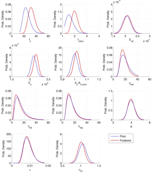
For consistency ten sequential runs of the updating algorithm were carried out, the re-sulting updated PDFs, along with the the prior PDFs, of these runs are shown in fig. 2.5. Significant changes in the parameters that influence the concrete tensile strength, namely fc and fctmo, can be noticed. This was expected since the displacement behavior
for reinforced concrete girders are strongly dependent on the tension stiffening behavior and, consequently, on the tensile behavior of the concrete. Also, when viewing these re-sults, it can be noticed that the random variable representing the yield strength was not updated in this process. Simulations were carried out considering this variable, however no noticeable changes were found. This was attributed to the fact that it is highly un-likely that the yield strength has any effect on the girder response for the measured load intensities. Table 2.2 summarizes the results of the simulations; it shows that, for most of the analyzed parameters, there was good repeatability in the updating procedure. Some subtle changes were found in the updated distributions for the random variables which control the degradation mechanisms, K and ν. With regard to these results it
this is that, simply put, the response of reinforced concrete structures are dependent on two main components: the concrete and the reinforcement. So the updating procedure is capable, at best, of determining the concrete and reinforcement properties for the concrete girder at the time of the test. If the degradation model consists on reinforcement corrosion, as is the case considered here, it is very difficult to infer if the reinforcement suffered corrosion or if its area is different from the specified nominal area. Furthermore, with a degradation model that considers a corrosion initiation time it is even more difficult to estimate the parameters based on a single point in time. For instance, given that one knows the initial reinforcement area and, through testing, determines the reinforcement area for a point in time, there still would be no way of knowing if this was the result of the initiation time being lower than expected or if the corrosion rate is higher than anticipated. Therefore, if the objective behind the testing is determining the occurrence and/or progress of the degradation mechanisms then, testing should be carried out at different ages of the structure.
In the present case study, in which test data is only available at one age of the structure, there is the possibility of improving these results by taking measurements of the carbon-ation front and using this informcarbon-ation to update the random variable K. By having a
better identifiedK it is easier to obtain an estimate for the corrosion rate ν through the
Figure 2.5.: Bayesian updating results based on the measured displacement data.
These two updating cases were, again, repeated ten times. Table 2.2 shows the mean and c.o.v’s of the random variables’ parameters (mean and standard deviation) for the three updating cases. The integration of the carbonation depth information results in significant changes in the distribution for the random variableK. However, during the different runs
of the updating algorithm with this data, the corrosion rate and reinforcement cover distributions showed significant variability. This is most likely attributed to difficulties in sampling algorithm when dealing with variables with low influence on the response in low likelihood cases. Also, even though we have data that better identifies theK random
Model Displacement Displacement & Phenolphthalein Displacement & No Degradation
Parameters Mean C.O.V. Mean C.O.V. Mean C.O.V.
fc(MPa) µ 34.12 5.7% 32.76 9.5% 32.85 3.6%
σ 6.07 16.8% 4.46 19.5% 5.79 8.4%
fctmo(MPa) µ 2.00 4.5% 1.97 10.3% 2.02 4.5%
σ 0.27 16.6% 0.20 34.5% 0.26 8.3%
Ec0(MPa) µ 2.13×10
4 2.8% 2.14
×104 3.7% 2.08
×104 2.7%
σ 1.74×10³ 16.0% 1.17
×103 20.8% 1.61
×103 9.5%
Es(MPa) µ 2.17×10
5 1.2% 2.17
×105 2.1% 2.16
×105 0.7%
σ 6.02×10³ 10.7% 5.19×10³ 14.5% 6.45×10³ 13.7%
As/Asnom µ 1.02 0.9% 1.03 1.1% 1.02 0.4%
σ 0.024 7.3% 0.018 24.7% 0.023 8.4%
cbot (mm) µ 19.53 9.3% 17.78 15.3% 17.98 6.1%
σ 6.51 16.1% 4.69 17.9% 6.15 12.1%
ctop(mm) µ 14.92 19.5% 14.39 27.0% 13.44 17.3%
σ 8.80 19.9% 6.25 30.1% 9.96 15.3%
clat(mm) µ 18.87 10.7% 16.70 34.5% 14.24 10.6%
σ 7.67 20.8% 6.02 34.4% 7.33 18.4%
K (mm·yr−1/2) µ 3.92 3.7% 1.84 7.7% -
-σ 0.35 12.2% 0.06 41.0% -
-ν(cm·yr−1) µ 8.82×10⁻³ 7.8% 8.68×10⁻³ 25.7% -
-σ 2.32×10⁻³ 10.4% 1.78
×10−3 35.7% -
-γDL µ 1.01 2.9% 1.02 6.8% 1.01 3.5%
σ 0.09 7.3% 0.07 18.4% 0.09 6.5%
Table 2.2.: Mean and coefficient of variation of the distribution parameters for the ran-dom variables obtained in the ten runs of the updating algorithm for the three consid-ered cases.
Age: 38 years
Prior
μ = 33540 kN.m σ = 3164 kN.m Updated w/ Displacements μ = 36875 kN.m
σ = 2778 kN.m
Updated w/ Displacements & No Degradation μ = 37547 kN.m σ = 2579 kN.m Updated w/ Displacements
& Phenolphthalein Tests μ = 37841 kN.m σ = 2514 kN.m
2.4.2. Model Updating Using Data from Multiple Tests
As commented earlier, the degradation mechanism based on reinforcement corrosion re-quires at least three points in time to be determined. With this objective, a set of testing scenarios were used to explore the potential of using testing data for change in structural response detection and updating of damage mechanism parameters. The testing scenar-ios, shown in Table 2.3, consider that testing is carried out∆tyears after the original test
and that a change in response, when compared to the original test, was recorded.
In the first scenario, no change in response was detected in the future tests carried out in five year intervals. This scenario does not allow to make any inference regarding the corrosion rate, however it does give some information regarding the carbonation coefficient (corrosion did not initiate for at least 10 years after the original test). Scenario II has tests carried out every ten years with no change in the first test and a 10% increase in the last test. For scenario III, the tests are carried out every five years, with displacements, respectively, 5 and 10% higher than the original. Comparing these two scenarios, it may be inferred that the corrosion initiation times are different, with corrosion initiating first in scenario III, and the corrosion rates are similar (10% change in response in a 10 year period). Finally, for scenario IV, testing is done ten year intervals with changes of 5 and 10% which implies a lower corrosion rate than scenarios II and III and an initiation time close to scenario III.
∆t(years) 5 10 20
Scenario Change in Response
I 0% 0%
II 0% +10%
III +5% +10%
IV +5% +10%
Table 2.3.: Scenarios considered for updating using three points in time.
The updating routine for each scenario used the combined likelihood of the data obtained in the three tests, resulting in a set of 30 observations. For simplicity and, also, taking into consideration the results obtained in the previous section, the uncertainty of the concrete cover was not considered. Therefore the nominal values were used in this analysis, which allowed for a better characterization of theK (carbonation coefficient) parameter.
Similarly as in the previous updating procedure, for each scenario, ten consecutive runs of the algorithm were carried out.
Table 2.4 shows the mean and c.o.v.’s of the distribution parameters for the updated random variables. From these results it can be seen that the model parameters, fc, fctmo, Ec0, Es, AS/Asnom, and γDL, do not show significant changes in the four considered
scenarios. For the carbonation constant,K, the results show, the lower values associated
Considering a reinforcement cover of 20 mm the initiation times for the four scenarios would, respectively, be 30.2, 28.5, 26.4, and 27.8 years. This shows that for this cover depth, changes in initiation time vary from 2 to 4 years, since the cross section has reinforcement layers with larger covers, it is reasonable to assume that changes of 5 years in the initiation time would not generate significant changes in theK values.
With regard to the corrosion rate,ν, scenarios II and III presented similar values, scenario IV showed lower values than the aforementioned scenarios. This is consistent with the information from the scenarios, since scenario IV showed only 5% increase in displacement in a 10 year period as opposed to a 10% increase in the two other scenarios for the same period. As already mentioned, scenario I does not allow to make any inferences on the corrosion rate.
To better evaluate the effects of this variable and of the updating process in the lifetime flexural behavior of the girder, a Monte Carlo simulation was run using the mean values for the distribution parameters shown in Table 2.4. For comparison, a simulation using the prior distribution information was also carried out.
Figure 2.7 shows the evolution, in terms of mean values of the ultimate bending moment,
Mu, during a timespan of 100 years. A relative damage was calculated by dividing the
obtained mean values of Mu at the different times by the initial value (t = 0 years),
Model Scenario I Scenario II Scenario III Scenario IV
Parameters Mean C.O.V. Mean C.O.V. Mean C.O.V. Mean C.O.V.
fc (MPa) µ 36.32 8.3% 34.43 7.5% 35.74 5.6% 34.31 11.6%
σ 5.34 19.0% 5.13 19.7% 5.37 14.1% 5.16 13.0%
fctmo(MPa) µ 1.80 8.1% 1.81 5.6% 1.75 5.0% 1.84 7.9%
σ 0.23 20.3% 0.25 20.3% 0.22 10.9% 0.22 15.5%
Ec0(MPa) µ 2.18×10
4 5.2% 2.20
×104 2.9% 2.18
×104 3.0% 2.11
×104 2.0%
σ 1.44×10³ 15.7% 1.36
×103 21.4% 1.49
×103 17.4% 1.45
×103 16.9%
Es(MPa) µ 2.25×10
5 1.3% 2.25
×105 0.6% 2.23
×105 1.0% 2.25
×105 1.4%
σ 5.36×10³ 11.7% 5.65
×103 23.9% 5.58
×103 22.1% 5.51
×103 15.9%
As/Asnom µ 1.04 1.3% 1.04 0.9% 1.03 0.9% 1.03 2.0%
σ 0.021 20.9% 0.021 16.9% 0.020 25.5% 0.021 15.1%
K (mm·yr−1/2) µ 3.64 1.8% 3.75 2.8% 3.89 2.3% 3.79 2.7%
σ 0.21 10.6% 0.20 21.2% 0.25 20.0% 0.26 19.2%
ν(cm·yr−1) µ 8.38×10⁻³ 15.2% 8.88×10⁻³ 10.1% 8.76×10⁻³ 6.4% 7.84×10⁻³ 15.9%
σ 2.43×10⁻³ 43.3% 1.86
×10−3 14.9% 2.07
×10−3 22.7% 1.91
×10−3 20.2%
γDL µσ 1.050.08 13.0%1.8% 0.081.03 27.8%5.1% 1.040.08 9.9%2.0% 0.091.07 17.1%4.7%
Table 2.4.: Mean values and coefficient of variation of the random variable parameters obtained in the ten runs of the updating procedure for the four considered scenarios.
Figure 2.7.: Curves showing: the mean values of the ultimate bending moment (Mu)
and the relative damage (Mu/M