Abs tract
Being motivated by the technological applications of bioabsorbable
polymeric materials in the fields of biomechanics and medicine,
this paper presents a simple but efficient extension of Lemaitre’s
elastoplastic damage model by incorporating a chemical-based (hydrolysis) degradation term. The aim is to allow the simulation of devices subjected to both mechanical and chemical enviro n-ments. The model applicability is tested by a set of numerical
finite-element examples. The encouraging results show expected
adequate coupling between the elastoplastic and chemical damag-es. Although the model is presently restricted to linear kinematics, the basic idea can be extended to finite strains.
Key words
Bioabsorbable polymers, elastoplastic damage, hydrolytic degrad a-tion
Simple extension of Lemaitre's elastoplastic damage
model to account for hydrolytic degradation
1 IN T R O D U C T IO N
Medical implants made of bioabsorbable polymeric materials have been comprehensively investi-gated as efficient substitutes for their metallic counterparts. Costs, mechanical behavior, and their ability of being absorbed by the body once their mechanical function has ceased are the main features that motivate the use of these polymers. Among the most used bioabsorbable polymers developed for surgical procedures, the most common are polyglycolic acid (PGA) and polylactic acid (PLA) copolymers.
The process of degradation of bioabsorbable implants is represented by the irreversible phe-nomenon called hydrolysis that comprises the progressive breakage of the chemical bonds of the polymeric net due to its contact with bodily fluids. During this process, an initial decrease in the molecular weight is observed, followed by a loss in mechanical performance; finally, a loss of mass is observed. Due to this sequential degradation, as the mechanical properties of the bioabsorbable devices worsen, stresses are progressively transferred to the healed new tissue formed around them. In this way, they are designed to abandon their mechanical functions before being fully
Ed uard o A . Fan cel l o a , b, * L e and ro P. Li n de nm e ye r a C arlo s R. M. Ro es l er a G e an V . S alm ori a c , b
aGRANTE—Group of Analysis and Mech. Design; Mech. Engineering Department bLEBm—Lab. of Biomechanical. Eng.; University Hospital
cCIMJECT—Plastic Molding Lab.; Mechanical Engineering Department Federal Univ. of Santa Catarina, Brazil. Received in 12 May 2013
In revised form 30 Jul 2013
Latin American Journal of Solids and Structures 11 (2014) 884-996
absorbed. This final absorption is the last step in the degradation process, which is found in bio-chemical reactions.
The hydrolytic degradation of the polymer depends on the intrinsic properties of the material, and it is related to the diffusion coefficient of water, degradation rate, body size, degree of crys-tallinity, and mechanical stress state.
Degradation can occur in the following two ways (Chen et al., 2011). In the polymer medium, if the diffusion of water is slower than the degradation, rate, then surface degradation is observed, which progresses from the surface to the core. Conversely, when the water diffusivity allows for a rapid soaking of the entire device, then bulk degradation is observed, which acts on all the mate-rial points almost simultaneously. In the context of the present work, we assume that the latter functions as the primary agent of degradation for the PGA and PLA polymers.
Several studies have been performed to investigate the behavior of bioabsorbable polymers considering the effects of hydrolysis and mechanical stresses. Not aiming to present a systematic review, we cite some examples below.
An early study by Miller and Williams (1984) revealed that the virgin material of PLA poly-mers used in surgical sutures was subjected to strain values between 25%and 50%of their rupture strain values. The stress relaxation after 14–21 days was evaluated, revealing that the rate of hydrolysis clearly increased with the magnitude of the applied strain. Chu (1985) reported a rela-tionship between the applied strain and the degradation rate of PLA fibers immersed in a solu-tion. When pre-stress was applied to the material in an aqueous medium, microvoids appeared, which increased the water penetration and accelerated the degradation process. Zhong et al. (1993) analyzed the influence of a strain value of 4%on the degradation parameters when using PGA and PLA suture fiberssoaked in a solution of water and hydrogen peroxide. After two weeks of immersion, they concluded that the degradation rate was considerably higher in the presence of strain than its absence. Smit et al. (2008) evaluated the effect of axial compressive loading on the degradation of a spine cage made of 70/30 poly(l,dl-lactic acid)(PLDLLA). The results showed that the mechanical resistance of the material was dependent on the load, temperature, and hu-midity. Soares et al.(2008, 2009, 2010) presented constitutive models for bioabsorbable polymers that underwent degradation under applied strain. They proposed a scalar field that described the local state of degradation (isotropic damage). This field is related to an evolution law that de-pends on the state of the strain/stress. Muliana et al. (2009) and Muliana and Rajagopal (2011,2012) analyzed the different relationships between hydrolytic degradation, viscoelastic be-havior, and water diffusion. Basic hypotheses suggest that the Young’s modulus of the material decreases with degradation. In a very recent paper, Khan and El-Sayed (2013) includes a damage-type internal variable within a variational viscoelastic model to account for degradation phenom-enon in stents. It is interesting to note that none of the above mentioned works consider the combined influence of the damages induced by mechanical and chemical sources. For example, it is possible to find this coupling in vascular stents, because these devices are subjected to severe mechanical action (plastic diametral expansion) during the implantation procedure.
Latin American Journal of Solids and Structures 11 (2014) 884-906
that this term depends on the stress state. The model combines the effects of elastic and plastic strains, mechanical damage, and chemical (hydrolytic) damage. Although this model is restricted to infinitesimal kinematics, it can be extended to finite deformations.
Section 2 presents a short but self-contained mathematical formulation of the model. The no-tation used in this section is obtained from the book by de Souza Neto et al. (2008) where certain details about the technical operations can be found.
Section 3 illustrates the behavior of the proposed model. To this end, a set of numerical tests are conducted to evaluate the single constitutive equation as well as its inclusion in finite-element examples. It is worth mentioning, however, that the results do not represent any particular iden-tified material, and the intention of these results is to demonstrate the capabilities of the pro-posed model. A final section is added to summarize the obtained results.
2 H Y D R O LY T IC -P LA ST IC D A M A G E M O D EL
Let us consider an isotropic damage variable that is split into two terms: the first is the classical ductile damage of the Lemaitre’s model and the other is called hydrolytic damage. While the evo-lution of the former is directly related to the existence of plastic strains, the latter is dependent on time (chemical action) and stress state. Now, let us define the conventional external and in-ternal state variables, namely, the total strain ε, plastic strain εp, equivalent plastic strainep, plastic damage dp, and hydrolytic damage dh. The elastic strain and total damage can be
de-fined as
εe =ε−εp, d =dp +dh, (1)
For simplicity, we assume that both plasticity and damage phenomena are isotropic in nature. In this case, the free energy can be additively decomposed into two contributions: the elastic po-tential e
y , depending on the elastic strain and scalar damage, and the plastic one ψp, depending
on the accumulated plastic strain εp
only:
ψ=ψ ε,ε p
,ε p
,d p
,d h
(
)
=ψe εe,d
(
)
+ψp( )
εp(2)
The elastic potential is related to the linear isotropic material and is dependent on the bulk modulus K and shear modulus G:
ρψe = 1−d
(
)
2
εe : D : εe =
(
1−d)
Gεde : εde+92 Kε
v 2 ⎛
⎝ ⎜⎜ ⎜
⎞
⎠ ⎟⎟
⎟⎟ (3)
In (3), D is the isotropic elasticity tensor, ε
v =tr[ε e
], the volumetric strain, and
ε
d e
=εe−εv
3 I, the deviatoric elastic strain. Considering the linear constitutive relationship it is
Latin American Journal of Solids and Structures 11 (2014) 884-996
ρψe = 1
2 1
(
−d)
σ : D −1: σ = 1
1−d
(
)
q2
6G+ p2 2K ⎛ ⎝ ⎜⎜ ⎜⎜ ⎞ ⎠ ⎟⎟
⎟⎟⎟=
(
1−d)
q 26G+ p2 2K ⎛ ⎝ ⎜⎜ ⎜⎜ ⎞ ⎠ ⎟⎟ ⎟⎟⎟ (4)
where p=1
3tr⎡⎣σ⎤⎦ is the hydrostatic pressure, s=σ −pI is the deviatoric stress, and q = 3J2(s)= 3
2s:s is the equivalent von Mises stress. Their relationships with the correspond-ing effective values are
σ = σ
1−d
(
)
=, s=s
1−d
(
)
, p=p
1−d
(
)
, q=q
1−d
(
)
(5)On the basis of thermodynamical principles, the conjugated forces can be obtained from the derivative of
ψ
with respect to the state variables:σ =ρ∂ψ
∂εe =(1
−d)D : εe,
χ =ρ ∂ψ
∂εp =
−σ, k=ρ∂ψ ∂εp =k(ε
p)
(6)
Yp =ρ∂ψ ∂dp =
−q
2
6G − p
2
2K, Y
h =ρ ∂ψ
∂dh =Y
p (7)
Yp is the energy release rate due to an increment in the plastic damage. The new conjugate force
Yh results in exactly the same conjugate value of Yp; however, this value is now related to the hydrolytic damage. Despite the fact that Yh and Yp share the same value by definition, both these variables are expressed separately.
The von Mises yield function is given by
Φ
(
σ,k,d)
= q 1−d(
)
−σy( )
k ≤0 (8)where σ
y(k) is the hardening law.
To define the evolution rules of the internal variables, a common formalism can be used to as-sume the existence of a dissipative potential Ψ which ensures the automatic satisfaction of the Clausius–Planck inequality (non-negative dissipation process) on the basis of its convexity proper-ties. In the present case, the potential Ψ is exactly the same as that of the Lemaitre’s damage model along with a new term Ψh:
Latin American Journal of Solids and Structures 11 (2014) 884-906
In (9), we distinguish the yield function Φ,plastic potential Ψ
p, and the (new) hydrolytic poten-tial Ψh. Since Ψ ≠ Φ, the flow model is nonassociative.
In our case, we use the simplified Lemaitre and Chaboche plastic potential (de Souza Neto et al., 2008):
Ψp(Yp)=H ε p−ε
D p
(
)
r(1−d)(1+s)
−Yp r ⎛ ⎝ ⎜⎜ ⎜⎜ ⎞ ⎠ ⎟⎟ ⎟⎟⎟
s+1
, H
( )
a = 1 if a>0 0 if a≤0⎧ ⎨ ⎪ ⎪ ⎩ ⎪ ⎪ (10)
where r and s denote the material constants. The Heaviside step function
H is used to incorpo-rate a plastic threshold ε
D
p for the accumulated plastic strain εp below which no plastic damage rate is allowed.
The evolution of the internal variables εp, εp, and
dp are intrinsically related to the plastic flow phenomenon and can be defined based on the dissipation potential Ψ as follows:
εp =γN, N =∂Ψ ∂σ =
∂Φ
∂σ = 1 (1−d)
3 2
s
s (11)
εp =γH, H =−∂Ψ
∂k =
−∂Φ
∂k =1 (12)
dp =γV, V =−∂Ψ
∂Yp =− ∂Ψp
∂Yp =
H
(
εp−εDp)
) (1−d)−Yp r ⎛ ⎝ ⎜⎜ ⎜⎜ ⎞ ⎠ ⎟⎟ ⎟⎟⎟ s (13)
The N, H, and V values defined in (11), (12), and(13), respectively, are associated with the direction of evolution of the internal variables, while the Lagrange multiplier rate γ accounts for their amplitudes.
In the present proposition, the hydrolytic damage is not dependent on the plastic flow, unless it is indirectly related through the stress state. Therefore, dh
is independent of γ. Moreover, the hydrolytic damage is a time-dependent process driven by the kinetics of the chemical reactions. In chemical kinetics, a classical expression that accounts for the degradation rate is given below (de Paula & Atkins, 2011, pp.1328):
d =k(1−d)n
k=Aexp −Ea
RT ⎛ ⎝ ⎜⎜ ⎜⎜ ⎞ ⎠ ⎟⎟ ⎟⎟ (14)
where k is a rate constant depending on the temperature T , activation energy E
Latin American Journal of Solids and Structures 11 (2014) 884-996
we assume that the value of k depends on the strain energy Yh. Then, following the structure of
(14), we define the evolution of dh as follows:
dh =−∂Ψ ∂Yh
=−∂Ψ
h
∂Yh = −Y
h
l +g
⎛ ⎝ ⎜⎜ ⎜⎜ ⎞ ⎠ ⎟⎟ ⎟⎟⎟ m
(d−1)n (15)
The hydrolytic dissipative potential consistent with (15) is then expressed as
Ψh(Yh)= l
(m+1)
−Yh
l +g ⎛ ⎝ ⎜⎜ ⎜⎜ ⎞ ⎠ ⎟⎟ ⎟⎟⎟ m+1
(1−d)n (16)
where l,m,g are material constants. The first simple expression arises when taking n=1, i.e., a first-order chemical reaction, which provides an evolution that is conceptually similar to that of Soares et al. (2009). An important value in (15) isgthat guarantees the existence of the degrada-tion rate even in the case of absence of stresses.
Although similar, the expressions in (13) and (15) behave significantly differently; in the case of the former, the damage rate increases when the damage itself increases, which is the opposite behavior of the latter. In (13), the damage evolution is a time-independent process since it follows the plastic multiplier γ; in (15), the hydrolytic damage is essentially dependent on the time scale of the chemical process.
2.1 Increm ental updating
The time integration of the previous equations over the time step t n,tn+1 ⎡
⎣ ⎤⎦ defines the correspond-ing incremental constitutive algorithm. Here, we use the standard full implicit elastic predictor– plastic corrector technique, and the presentation is similar to the procedures shown in de Souza Neto et al. (2008) and Simo and Hughes (1998). We consider the set of state variables
ε
n,εn
p
,εn
p
,dn
p
,dn
h
{
}
at time tn(which is completely known) as well as the total strainε
n+1 =εn+Δε at time tn+1. The increment of the plastic deformation and damage comes from (11–15) and Δγ=Δt γ:
ε
n+1 p =ε
n p+
ΔγN
n+1, Nn+1 = 1
1−dn+1
(
)
3
2 s
n+1 s
n+1
(17)
dn+1 =dnp+1+dnh+1 =dn+Δdp +Δdh (18)
Δdp = Δγ
(1−dn+1)
−Ynp+1
Latin American Journal of Solids and Structures 11 (2014) 884-906
Δdh =Δt(1−d n+1)
−Ynh+1
l +g ⎛ ⎝ ⎜⎜ ⎜⎜⎜ ⎞ ⎠ ⎟⎟ ⎟⎟ ⎟ m (20)
In (20), the evolution law of (15) was substituted after consideringn =1. The computation of the
elastic strain and corresponding effective stresses is given by ε
dn+1
e =ε
dn+1− εn p +
ΔγN n+1
(
)
, εvn+1
e =ε
vn+1 (21)
s
n+1 =2G εdn+1− εdn p
+ΔγN n+1
(
)
(
)
, sn+1=(1−dn+1)sn+1 (22)
pn+1 =Kεevn+1 =Kεvn+1, pn+1 =(1−dn+1)pn+1 (23)
The consistence condition in (8) at t
n+1 takes the form
Φn+1 =q
n+1−σy k(εn p +Δγ)
(
)
≤0 Δγ≥0, Φn+1Δγ=0 (24)2.2 Elastic predictor
(
Φn+1≤0)
In this step, we assume that the strain increment is purely elastic, i.e., Δγ=0. In this case, the so-called trial quantities can be defined as
ε n+1 etr =ε
n+1−εn p, ε
n+1 ptr =ε
n
p (25)
s
n+1 tr =2Gε
dn+1 etr , p
n+1 tr =Kε
vn+1 etr , q
n+1 tr = 3
2
s
n+1 tr : s
n+1
tr (26)
−Y n+1
ptr = qn+1 tr
(
)
26G +
pn+1
tr
(
)
22K
(27)
Since Δγ=0, the damage increment, if it exists, can be attributed only to the hydrolysis
phe-nomenon. Therefore,
dn+1 tr =d
n p+d
n+1
htr (28)
dnhtr+1=dnh+Δt (1−dnp−dnhtr+1) −Yn+1 ptr
Latin American Journal of Solids and Structures 11 (2014) 884-996
Isolating d
n+1 htr
from (29), we get
dnhtr+1=
dnh +Δt(1−dnp) −Yn+ptr1
l +g
(
)
m1+ −Yn+1 ptr
l +g
(
)
mΔt(30)
which allows the computation of s n+1 tr
, pntr+1, and qntr+1 as follows:
s n+1
tr =(1−d n+1
tr )s n+1
tr , p n+1
tr =(1−d n+1
tr )p n+1
tr , q n+1
tr =(1−d n+1
tr )q n+1
tr (31)
Finally, the yield function can be evaluated for the trial values as follows:
Φn+1
tr :=q n+1
tr
−σ
y k(εn+1
tr )
(
)
(32)If the condition Φn+1tr
≤0 is satisfied, then the step is purely (damage) elastic
(
Δγ=0)
and thevariables are updated using the corresponding trial values:
⋅
( )
n+1 :=( )
⋅n+1 trOtherwise, Φn+1
tr >0; then, a plastic increment
Δγ>0 exists. In this case, the new updated
variables are determined to satisfy the condition Φn+1 =0, which corresponds to the plastic
cor-rector step.
2.3 Plastic corrector
(
Δγ>0)
In this step, the following set of equations is solved:
εdn
+1 e
=εdn
+1 etr
− Δγ (1−dn
+1) 3 2 s n+1 sn +1 (33)
εnp+1=ε n
p +
Δγ (34)
dn+1 =dn+ Δγ
(1−dn+1)
−Ynp+1
r ⎛ ⎝ ⎜⎜ ⎜⎜⎜ ⎞ ⎠ ⎟⎟ ⎟⎟ ⎟ s
+Δt(1−d n+1)
−Ynh+1
l +g ⎛ ⎝ ⎜⎜ ⎜⎜⎜ ⎞ ⎠ ⎟⎟ ⎟⎟ ⎟ m (35)
Φ=q
n+1−σy k(εn+1 p
Latin American Journal of Solids and Structures 11 (2014) 884-906
From (33), it is possible to write
qn+1 =q
n+1
tr
− 3GΔγ
(1−dn+1) (37)
which may be substituted in (35). Similarly, replacing (34) in (36), the system is reduced to the following pair of equations:
Φ=q
n+1 tr
− 3GΔγ
(1−dn+1)−σy k(εn p +
Δγ)
(
)
=0 (38)dn+1 =dn+
Δγ (1−dn+1)
−Ynp+1
r ⎛ ⎝ ⎜⎜ ⎜⎜⎜ ⎞ ⎠ ⎟⎟ ⎟⎟ ⎟ s
+Δt(1−d n+1)
−Ynh+1
l +g ⎛ ⎝ ⎜⎜ ⎜⎜⎜ ⎞ ⎠ ⎟⎟ ⎟⎟ ⎟ m (39) where
−Ynp+1 =−Ynh+1 = 1 6G
qntr+1− 3GΔγ (1−dn+1)
⎡ ⎣ ⎢ ⎢⎢ ⎤ ⎦ ⎥ ⎥⎥ 2 +
pn2+1
2K (40)
Isolating wn
+1=1−dn+1 from (38) and introducing it in (39), a single nonlinear equation in Δγ can be obtained:
F(Δγ)=wn+1(Δγ)−wn + Δγ wn+1(Δγ)
−Yn+p 1 r ⎛ ⎝ ⎜⎜ ⎜⎜⎜ ⎞ ⎠ ⎟⎟ ⎟⎟ ⎟ s (41)
+wn+1(Δγ) −Yn+1 h
l +g ⎛ ⎝ ⎜⎜ ⎜⎜⎜ ⎞ ⎠ ⎟⎟ ⎟⎟ ⎟ m ⎡ ⎣ ⎢ ⎢ ⎢ ⎢ ⎤ ⎦ ⎥ ⎥ ⎥ ⎥
Δt =0, (42)
Note that this expression differs from the classical Lemaitre’s model in the last term of (41). The solution of this single nonlinear equation is obtained by using the Newton–Raphson method. In de Souza Neto et al. (2008), a convenient initial value Δγ(0) is proposed as follows:
Δγ(0)=
qn+tr1−σy
( )
εnp ⎡⎣⎢ ⎤⎦⎥wn
3G
Latin American Journal of Solids and Structures 11 (2014) 884-996
εn+p 1 =εnp +Δγ,
pn+1 =wn+1(Δγ) pn+tr1, qn+1=wn+1(Δγ) qn+tr1−3GΔγ
s
n+1 = wn+1(Δγ)−
3GΔγ
qn+tr1
⎡ ⎣ ⎢ ⎢ ⎢ ⎤ ⎦ ⎥ ⎥ ⎥ s n+1
tr , σ
n+1 =sn+1+pn+1I
ε n+1
p =ε
n
p + Δγ
1−dn+1
(
)
3 2 s n+1 s n+1Finally, the above algorithm σ
n+1 =σˆ εn+1,εn,εn p,d
n
(
)
of the incremental constitutive problem yields the derivative.D=
∂σ
n+1
∂ε
n+1
providing the consistent tangent elastoplastic tensor. Clearly, a closed expression of this deriva-tive is obtainable, but not included in this paper.
3 N U M ER IC A L EX A M P LES
In this section, we present a set of examples aiming to demonstrate the behavior and applicability of the proposed model. The material parameters used, however, do not correspond to any specific material and are taken just as examples. It is worth mentioning that the parameters related to the hydrolytic damage are clearly dependent on the unit of time, since it is a phenomenon that is significantly influenced by the time scale in which the chemical phenomenon occurs. Here, since no identification process was considered, the time unit used will be generically called a “day.” The values shown in Table 1 were used for all the further studied cases and are intended to resemble those of a polymeric material.
3.1 U niaxial tensile test
3.1.1 Strain-controlled tensile test: Case 1
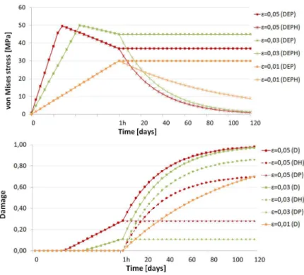
In this case, we consider a single material point subjected to an axial tensile test controlled by axial strain. Three loads are applied that are linearly varied from zero to the maximum strain values of 0.05, 0.03, and0.01 during a time interval of [0,120] days. Figure 1 shows the curves of the von Mises stress versus time and damage versus time for all the load conditions, which can be used to compare the behavior of the proposed plastic-hydrolytic damage model (DEPH) with a purely plastic damage (DEP) model. As expected, the hydrolytic damage curves exhibit higher values in the cases with higher stress values. In the case of the maximum strain of 0.01, no
Latin American Journal of Solids and Structures 11 (2014) 884-906
Figure 1 von Mises stress versus time and damage (D: total; DH: hydrolytic; DP: plastic) versus time (Case 1).
Latin American Journal of Solids and Structures 11 (2014) 884-996
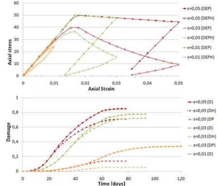
3.1.2 Strain-controlled tensile test: Case 2
In this example, a similar tensile test is conducted; however, we consider that the maximum strain is applied for a short interval of 1/24 day and then maintained constant for up to 120 days. Figure 2 shows the curves of the von Mises stress versus time and damage versus time for all the load conditions. Again, the higher the load, the higher is the initial damage rate. During the initial loading (1/24 day), the hydrolytic damage is imperceptible and only plastic damage is visible.
3.1.3 Strain-controlled tensile test: Case 3
The same maximum strains are linearly applied during the first 60 days and then linearly un-loaded during the next 60 days. Figure 3 shows the stress component (σ
x) versus strain curve and damage versus time curve.
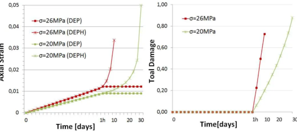
3.1.4 Stress-controlled tensile test: Case 4
Similarly to the previous cases, in this case, the tensile test is controlled by the applied axial stresses with maximum values of 20MPa and 26MPa that are linearly applied during a short time step of 1/24 day and then maintained constant. Figure 4 shows the curves of strain versus time and damage versus time. Note that in both these instances, the applied loads are less than the plastic yield value of 50MPa. However, due to hydrolytic damage, plasticity is finally
achieved, thereafter driving the material point to collapse.
Latin American Journal of Solids and Structures 11 (2014) 884-906
3.1.5 Stress-controlled tensile test: Case 5
In this case, the stress values of 18MPa and 20MPa are linearly applied for 60 days and unload-ed in the next 60 days. Figure 5 shows the curves of the von Mises stress versus time and damage versus time. Again, in both these instances, the applied loads are less than the plastic yield value of 50MPa. For the load of 20MPa, hydrolytic damage occurs before the unloading and collapse.
For the load of 18MPa, despite the increasing damage, unloading is faster and the material point
is able to withstand the load.
Figure 4 Axial strain versus time and damageversus time (Case 4).
Figure 5 Axial strain versus time and damage versus time (Case 5).
3.2 A xisym m etric sam ple
3.2.1 D isplacem ent-controlled test: Case 6
Latin American Journal of Solids and Structures 11 (2014) 884-996
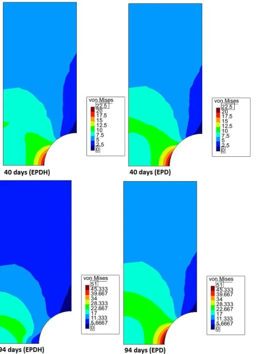
The prescribed displacement increases linearly from zero to 0.15mm within the time interval
of [0,120] days. Figures 7 and 8 show the von Mises stress distribution and damage distribution for the two instances: 40 and 94 days, respectively. From Figure7, it is evident that strong re-laxation occurs in the instance when hydrolysis is taken into account. Further, the stress distribu-tion changes significantly; the maximum value emanates from the notch and appears in the inte-rior of the domain.
Fi
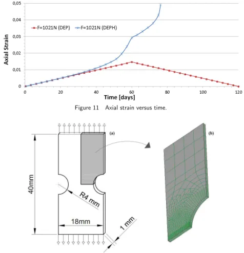
Fi Figure 6 Axial tensile specimen and simulated mesh.
3.2.2 Force-controlled test: Case 7
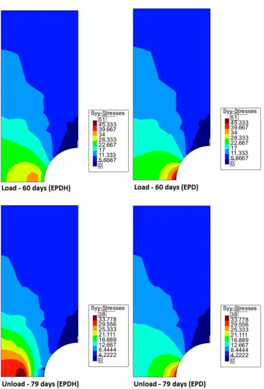
The same sample as that used in Case 6 is subjected to a controlled axial force that grows linear-ly from zero to 1021N within the time interval of [0,120] days. After that, progressive unloading is undertaken at the same rate, reaching (theoretically) zero value at 120 days. This maximum force value was set up so that the virgin material could reach the maximum stress value of 50 MPa. Figures 9 and 10 show the von Mises stress distribution and damage distribution for two different times: 60 and 79 days, respectively. A behavior similar to that in the previous case is evident; due to the presence of hydrolysis, the stresses at the notch relax and the maximum von Mises stress value is found to exist in the interior of the domain.
It is noteworthy that since this is a force-controlled test, the sample cannot withstand the load if hydrolysis is considered. Figure 11 shows the axial strain at the notch in the sample. The un-loading at 60days for both the instances is clearly visible; however, since hydrolysis keeps
damag-ing the sample, plastic collapse is achieved at 79 days (Figure 15, loss of convergence).
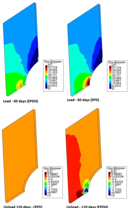
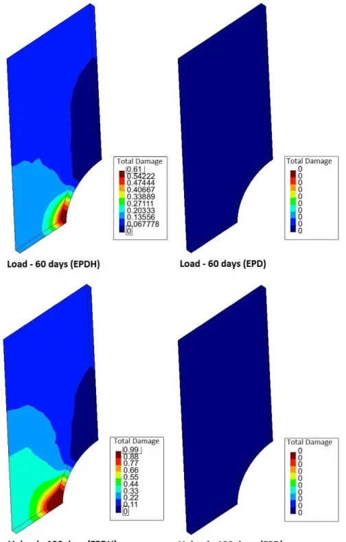
3.2.3 Plate Sam ple: Case 8
In this case, we simulate a plate sample using the 8-node Lagrangian brick elements (Figure 12), which can be used to represent a 3D sample discretized with solid elements. In this case, a dis-tributed force is progressively applied on the top surface of the plate; the maximum value of
Latin American Journal of Solids and Structures 11 (2014) 884-906
load value at 120 days. Figures 13 and 14 show the distribution of the axial stress component
σ
yand the damage at two times: 60 and 120 days. As expected, the behavior is similar to that in the cylindrical case; the damage due to hydrolysis significantly modifies the stress distribution at the notch. During the unloading phase, it is possible to visualize the competition between the remaining resistance of the specimen and the unloading tensile force. At the end of the process, the local compressive forces remain near the notch region for the hydrolytic model.
Latin American Journal of Solids and Structures 11 (2014) 884-906
Latin American Journal of Solids and Structures 11 (2014) 884-906
Figure 11 Axial strain versus time.
Figure 12 Tensile specimen and simulated mesh.
4 FIN A L R E M A R K S
Being motivated by the technological applications of bioabsorbable polymeric materials, the ob-jective of this paper is the proposal of a simple extension of the classical Lemaitre’s elastoplastic damage model that includes the representation of damage induced by chemical phenomena (such as hydrolytic degradation). In a simple and efficient manner, this model demonstrates the rela-tionship between the damage evolution due to mechanical and chemical actions. The applicability of the model is analyzed by undertaking a set of numerical tests. Although the model is presently restricted to linear kinematics, the idea can be extended to finite strains.
A set of specific technical remarks are highlighted below:
• Hydrolytic damage interferes with all the state variables at all the material points subjected to chemical activity. Moreover, this damage appears even in the absence of stresses due to the material parameter g.
Latin American Journal of Solids and Structures 11 (2014) 884-996
• Mechanical damage is independent of time since it undergoes plastic evolution. Hydrolytic damage is essentially dependent on the time scale of the chemical process.
• The results of the investigated examples are consistent with the expectations for different situations. At the beginning of the load, the evolution of the damage is driven only by the hydrolysis process. When the material reaches the plastic flow, the degradation rate increases significantly due to the coupled action between both the hydrolytic- and plasticity-driven damages.
Latin American Journal of Solids and Structures 11 (2014) 884-906
Latin American Journal of Solids and Structures 11 (2014) 884-996
• In the cases when the material point is subjected to a strain-controlled process, the expected stress relaxation depends on the degradation rate. On the other hand, when the material is subjected to a stress-controlled process, the degradation forces the material to undergo plastic flow followed by collapse.
• In all the investigated cases, hydrolytic damage increased faster than elastoplastic damage. This, however, should be attributed to the arbitrary choice of the material parameters in the examples.
• The proposition in (2) regarding free energy decoupling, although conventional, cannot be considered a unique alternative. For example, in the studies of Brünig (2002, 2004) and the references therein, the damage follows a kinematic description similar to that of plastic strains and the free energy is additively decoupled in elastic (reversible) and inelastic (damage and plastic) contributions. This approach would certainly modify the definitions of the conjugate forces Yh and Ypin (7). In spite of these alternatives, the present work has aimed to main-tain the same structure of the original Lemaitre’s elastoplastic damage proposition (Lemaitre, 1985).
Summarily, it is worth mentioning that the actual representation of a bioabsorbable material deserves attention in several aspects that have not been considered here. Among others, one such aspect is the modification of the material properties due to the chemical actions: in the present simple damage model, the yield limit and elastic modulus of the virgin material decrease as long as the damage increases. The process of aging due to chemical actions may produce embrittle-ment and/or stiffening of the elastic behavior instead of the softening action observed in the pre-sent case.
Acknowledgm ents
The authors would like to thank the Brazilian agencies CNPq, CAPES and FINEP for the fi-nancial support offered for this research.
References
Y. Chen, S. Zhou, and Q. Li(2011). Mathematical modeling of degradation for bulk-erosive polymers: Applica-tions in tissue engineering scaffolds and drug delivery systems. ActaBiomaterialia, 7:1140-1149.
C.C. Chu (1985).Strain-accelerated hydrolytic degradation of synthetic absorbable sutures. Surgical research, recent developments. Proceedings of the First Annual Scientific Session of the Academy of Surgical Research, 111-115.
M. Brünig (2002). Numerical analysis and elastic-plastic deformation behavior of anisotropically damaged sol-ids. International Journal of Plasticity, 18:1237-1270.
M. Brünig (2004) An isotropic continuum damage model: Theory, and numerical analyses. Latin American Journal of Solid and Structures, 1: 185-218.
E. A. de Souza Neto, D. Peric, and D. R. J. Owen (2008). Computational methods for plasticity: Theory and applications. WILEY.
Latin American Journal of Solids and Structures 11 (2014) 884-906
J. Lemaitre (1985). Coupled Elasto-plasticity and damage constitutive equations. Com. Meth. Appl. Mech. Engng, 51:31-49.
N.D. Miller and D.F. Williams (1984). The in vivo and in vitro degradation of poly(glycolicacid) suture mate-rial as a function of applied strain. Biomatemate-rials, 5:365-368.
A. Muliana, K.R. Rajagopal, and S.C. Subramanian (2009). Degradation of an elastic composite cylinder due to the diffusion of a fluid. Journal of Composite Materials, 43(11):1225-1249.
A.H. Muliana and K.R. Rajagopal (2011).Changes in the response of viscoelastic solids to changes in their in-ternal structure. Acta Mechanica, 217(3-4):297-316.
A. Muliana and K.R. Rajagopal (2012). Modeling the response of nonlinear viscoelastic biodegradable poly-meric stents. International Journal of Solids and Structures, 49(7-8):989-1000.
J. V. Simo and T. J. R. Hughes (1998). Computational Inelasticity. Springer.
T. H.Smit, T A P Engels, P I J M Wuisman, and L E Govaert (2008). Time-dependent mechanical strength of 70/30 poly(L,DL-Lactide) shedding light on the premature failure of degradable spinal cages. Spine, 33:14-18.
J. S. Soares, J. E. Moore, JR., and K. R. Rajagopal (2008).Constitutive framework for biodegradable polymers with applications to biodegradable stents. ASAIO Journal, 295-301.
J. S.Soares, K. R. Rajagopal, and J. E. Moore Jr. (2010).Deformation-induced hydrolysis of a degradable pol-ymeric cylindrical annulus. Biomechanics and Modeling in Mechanobiology, 9:177-186.