Penetrance rate estimation in autosomal dominant conditions
Paulo A. Otto
1and Andréa R.V.R. Horimoto
21
Departamento de Genética e Biologia Evolutiva, Instituto de Biociências, Universidade de São Paulo,
São Paulo, SP, Brazil.
2
Laboratório de Genética e Cardiologia Molecular, Faculdade de Medicina, Instituto do Coração,
Universidade de São Paulo, São Paulo, SP, Brazil.
Abstract
Accurate estimates of the penetrance rate of autosomal dominant conditions are important, among other issues, for optimizing recurrence risks in genetic counseling. The present work on penetrance rate estimation from pedigree data considers the following situations: 1) estimation of the penetrance rate K (brief review of the method); 2) con-struction of exact credible intervals for K estimates; 3) specificity and heterogeneity issues; 4) penetrance rate esti-mates obtained through molecular testing of families; 5) lack of information about the phenotype of the pedigree generator; 6) genealogies containing grouped parent-offspring information; 7) ascertainment issues responsible for the inflation of K estimates.
Key words:penetrance rate, maximum likelihood method, recurrence risks, genetic counseling.
Received: February 1, 2012; Accepted: May 23, 2012.
Introduction
Human autosomal dominant diseases are extremely rare conditions in which affected individuals are heterozy-gotes. Many of these heterozygous genotypes exhibit the phenomenon of incomplete penetrance. For this set of rare conditions the penetrance rate is therefore understood as the probability of a heterozygote presenting the disease (or, at least, presenting a minimum number of signs and symp-toms that enable his/her identification as a carrier of the del-eterious allele). Other details, as well as a full review of the subject can be found in Horimoto and Otto (2008). Accu-rate estimates of the penetrance value K are important not only for determining genetic disease risks in families with segregating cases of autosomal dominant disorders, but also for performing linkage studies. Crude penetrance esti-mates can be derived by dividing the observed number of diseased (penetrant) individuals by the number of obligate carriers (penetrant as well as obligate non-penetrant, that is, normal individuals with several affected offspring or nor-mal individuals with affected parent and child). Presently the penetrance parameter can be estimated on a routine ba-sis by computer programs that perform segregation analy-sis or the estimation of linkage based on complex pedigree structures that cannot be expressed in closed form, such as the classical S.A.G.E. (S.A.G.E., 2009) and LINKAGE (Lathropet al., 1985) programs.
Rogatkoet al.(1986) provided a simple but efficient methodology for dealing with the problem, but neither their solution nor more complex alternatives, such as the above-mentioned computer programs, take into account many of the details we discuss here. These concern specificity and heterogeneity issues (section 3), penetrance rate estimates from families undergoing molecular testing (section 4), lack of information about the phenotype of the pedigree generator (section 5), genealogies containing grouped par-ent-offspring information (section 6), and ascertainment is-sues responsible for the inflation of K estimates (section 7). In section 1 we briefly review the method for estimating the penetrance rate from pedigree data, and in section 2 we make a digression on the determination of the exact credi-ble interval for this estimate.
(1) Method for Estimating the Penetrance
Rate K
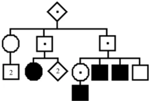
More details on the method described below are found in the original paper by Rogatkoet al. (1986) and Horimotoet al.(2010). The first step of the method consists in trimming or filtering the pedigree information, that is, re-placing the original pedigree with one containing only indi-viduals that are informative or relevant with respect to penetrance estimation. Expressions like trimming and trim-med seem to be more appropriate, but we shall keep the no-menclature coined originally by Rogatkoet al.(1986). As an example we will consider the hypothetical filtered pedi-gree shown in Figure 1, with several individuals affected by www.sbg.org.br
Send correspondence to Paulo A. Otto. Departamento de Genética e Biologia Evolutiva, Instituto de Biociências, Universidade de São Paulo, Caixa Postal 11461, 05422-970 São Paulo, SP, Brazil. E-mail: otto@usp.br.
a rare autosomal dominant condition. The individual of the first generation is the genealogy or pedigree generator. The symbols marked with a point indicate obligate normal (non-penetrant) heterozygous carriers of the gene, and the darkened symbols represent affected (penetrant) heterozy-gotes.
The filtered pedigree contains four affected individu-als, four normal obligate carriers, three normal offspring of obligate carriers, and one tree of normal individuals de-scendants from an obligate carrier (one normal female with two normal male offspring, shown at the leftmost position of the pedigree). LettingKbe the penetrance rate value, the probabilities associated with each of these four different structures are, respectively,K/2, (1-K) in the case of the pedigree generator, or (1-K)/2 in the case of the other three normal obligate carriers, (2-K)/2, and {1/2 + (1-K)/2. [(2-K)/2]2}.
The likelihood function, that is the probability of oc-currence of the pedigree conditional to the observed struc-tures occurring in it, is derived from the quantities associ-ated with these structures. In the present case, by neglecting constant values unimportant in the maximization procedure that will follow, the likelihood function takes the form p =
K4(1-K)4 (2-K)3[4+(1-K)(2-K)2]. By solving the equation dP/dK= 0 (or, more conveniently, dL/dK= dlog(P)/dK= 4.log(K)+4.log(1-K)+3.log(2-K)+log[4+(1-K)(2-K)2] = 0), we obtain the maximum likelihood estimate of the pene-trance valueK, which for this family takes the value of 0.418.
Heterozygosis probabilities and the corresponding risks for the offspring of all individuals of the filtered pedi-gree can then be determined without difficulties. Obligate carriers (known non-penetrant carriers and affected pene-trant heterozygotes) have genotype Aa and the risk for their offspring is simply R1=K/2 = 0.418/2 = 0.209, or approxi-mately 21%, for the above shown example. The probability of heterozygosis for normal individuals born to obligate carriers (three of which occur in the family used as exam-ple) is taken directly from the quantity (2-K)/2 = 1/2+(1-K)/2 as P(het) = [(1-K)/2]/ [(2-K)/2] = (1-K)/(2-K) = 0.582/1.582 = 0.368. The probability of affected offspring for these individuals is then R2= (1-K)/(2-K).K/2 = 0.368 x
0.209 = 0.077, or approximately 8%. The heterozygosis probabilities for all three individuals of the single tree of normal individuals occurring in the worked pedigree can be obtained from the term {1/2 + (1-K)/2.[(2-K)/2]2} by apply-ing simple Bayesian reasonapply-ing, or by means of computer programs. In an earlier work (Horimotoet al., 2010) we de-scribe two self-contained computer programs that perform most calculations necessary to estimate the penetrance rate. These are the programsPenCalc for WindowsandPenCalc Web, which can be obtained free of charge from the web page http://www.ib.usp.br/~otto/software.htm. Both pro-grams are described in detail in the above mentioned article as well as in the PDF-guide included in the zipped file of the program PenCalc for Windows.
(2) Construction of Exact Credible Intervals for
K Estimates
Rogatkoet. al. (1986) also used an exact credible in-terval associated with a givenKestimate. This interval can be obtained by finding the area that corresponds to a given proportion (v.g., 95%) of the total area under the graph of the likelihood function. Mathematically, the problem is re-duced to integrating the function y = f(K) between two lim-its a and b with the same ordinate value [f(K= a) = f(K= b)], so thatòa,b[f(K)dK]/ò0,1[f(K)dK] = 0.95, an operation which can be accomplished by simple computer programs using numerical integration techniques such as Romberg’s oscullatory method. The lower and upper limits of the exact 95% credible interval for the estimateK= 0.418 of the ex-ample above are 0.163 and 0.725, respectively. This credi-ble interval is so large that it might seem to be impractical in a clinical setting. The reason for this particular extreme range is that it was derived from the few data of the small family used as example. In practice, larger pedigrees are usually used. The ideal situation is one where several pedi-grees of the same condition are available for analysis, and the pooled data are used to perform the calculations of the penetrance rate and of its 95% credible interval. For instance, from the analysis of 21 different published pedi-grees on the autosomal dominant ectrodactyly-tibial hemi-melia syndrome, penetrance estimates and their correspon-ding credible intervals varied from 0.191 (0.044-0.574) to 0.750 (0.329-0.973), while the global (pooled) penetrance value estimate was 0.392, with a 95% credible interval of 0.339 to 0.447 (Horimoto, 2009).
(3) Specificity and Heterogeneity Issues
Another point that merits discussion is whether theK
value is specific for the family in which the disease segre-gates or for the condition itself, independently from the fam-ily. The non-penetrance of a genetic trait is assumed to represent the lack of its phenotypic manifestation exclu-sively or predominantly due to environmental factors (Mur-phy and Chase, 1975; Praxedes and Otto, 2000) or random
genetic and epigenetic processes linked to the disease locus. Of course penetrance can also be affected by a number of events that include the epistatic action of modifying genes and even temporal modifications of diagnostic criteria. Therefore, to a certain extent, penetrance estimates might be family-specific. Another complicating issue is that geneti-cally heterogeneous conditions can be merged in the pooling process. Nevertheless, since the statistical credible intervals of isolated pedigrees usually are large, pooled estimates of the parameter should be preferred, unless statistical tests dis-close the existence of great amounts of heterogeneity among penetrance estimates from various pedigrees.
(4) Penetrance Rate Estimates from Families
Undergoing Molecular Testing
In this section we discuss the comparison of estimates obtained from families without molecular testing as to those for which DNA testing has been used for classifying non-penetrant heterozygotes and normal homozygotes. In the lat-ter case, if molecular testing discloses all non-penetrant het-erozygotes inside normal trees of individuals descending from obligate carriers, and if there aren1affected (penetrant) individuals andn2non-penetrant heterozygotes in the family, the likelihood function reduces to L = log(P) =
n1.log(K)+n2.log(1-K). The maximum likelihood estimate is then K = n1/(n1+n2), with binomial sampling variance of var(K) =K(1-K)/(n1+n2). This would be an ideal situation in which, besides providing a better estimate ofK, the corre-sponding 95% credible interval of the penetrance value thus evaluated will be much smaller than the one provided by the analysis of the family without DNA testing.
(5) Lack of Information about the Phenotype of
the Pedigree Generator
In some published pedigrees there is a lack of pheno-typic information about the genealogy generator (affected or non-affected?). Furthermore, the likelihood function P may not include the parameterKor (1-K) corresponding to the genealogy generator.
In order to evaluate whether the inclusion of the pedi-gree generator significantly alters thisKestimate, it is not necessary to repeat the calculations for the two configura-tions possible (penetrant or non-penetrant common ascen-dant), because the likelihood function P, derived without information on the pedigree generator, is correct, and thus cannot be improved. In fact, if one wants to refer to the ped-igree founder, one can say that she/he was affected with probabilityKand unaffected with probability (1-K). The re-sulting likelihood isKP + (1-K)P = P.
(6) Genealogies Containing Grouped
Parent-Offspring Information within Trees of Normal
Individuals Descending from Obligate Carriers
Certain published pedigrees present grouped parent-offspring trees of normal individuals, without informing the corresponding offspring numbers of all individuals in a given sibship, as is the case of the pedigree with cases of the ectrodactyly-tibial hemimelia syndrome (Majewskiet al., 1985) shown in Figure 2. This tree of normal individuals represented by individuals II.8 to II.11 and III.14 to III.28 does not detail individual offspring numbers, and only the total number of 15 is given.
Incomplete pedigree information is a simple but inter-esting problem in combinatorial analysis that can be straightforwardly solved by means of the theory of differ-ence operators. Table 1 lists the numbers of possible gene-alogy structures for a case of incomplete parent-offspring information as a function of both parent and offspring num-bers. Therein, with four parents, the number of possible structures is given byy4(n) = (n+1)2+ (n+1)n(n-1)/6, where n is the total offspring number of the four parents. For
n= 15, the outcome is y4(15) = 816 of such structures. For each combination {i,j,l,m} of offspring number the likelihood function of the whole tree is:
K4(1-K)2(2-K)5{1/2+(1-K)/2[(2-K)/2]9}{1/2+(1-K)/2 .[(2-K)/2]i}{1/2+(1-K)/2.[(2-K)/2]j}{1/2+(1-K)/2.[(2 -K)/2]l}{1/2+(1-K)/2.[(2-K)/2]m},
wherei,j,l, andmare the unknown numbers of children for each of the individuals II-8, II-9, II-10, and II-11,
respec-Figure 2- Pedigree containing a grouped tree of normal individuals (mod-ified from Majewskiet al., 1985).
Table 1- Numbers of possible genealogy structures for the case of incom-plete parent-offspring information.
Off-spring number
Parent number
1 2 3 4 5 6 7 8
0 1 1 1 1 1 1 1 1
1 1 2 3 4 5 6 7 8
2 1 3 6 10 15 21 28 36
3 1 4 10 20 35 56 84 120
4 1 5 15 35 70 126 210 330
5 1 6 21 56 126 252 462 792
6 1 7 28 84 210 462 924 1716
7 1 8 36 120 330 792 1716 3432
8 1 9 45 165 495 1287 3003 6435
tively. In a population of approximately stable size, the av-erage offspring number per couple does not differ from two and it is known that the number of children per couple ade-quately fits a Poisson distribution g(x) = e-22x/x! .
If each possible configuration is weighed by its prob-ability (according to the Poisson distribution for the num-ber of children per couple), this gives a credible interval on K in a straightforward manner. This can be achieved as fol-lows using the function:
P(i,j,l,m) =K4(1-K)2(2-K)5{1/2+(1-K)/2[(2-K)/2]9} {1/2+(1-K)/2.[(2-K)/2]i} e-22i/i!{1/2+(1-K)/2. [(2-K)/2]j}e-22j/j!{1/2+(1-K)/2[(2-K)/2]l}e-22l/l!{1/2 +(1-K)/2[(2-K)/2]m}e-22m/m!,
and considering all 816 possible configurations referred to above. For each configuration one can then obtain not only aKijlmestimate but also its exact 95% credible inter-val. Estimates for the penetrance valueK, as well as for its exact 95% lower and upper credible limitsLKandUK, corresponding to the given tree structure can be straight-forwardly obtained by averaging the estimatesKijlm, as well as those for the lower and upper limitsLKijlm and UKijlm, as:
K=S(Kijlm.e-22i/i!.e-22j/j!.e-22l/l!.e-22m/m!) /S(e-22i/i! . e-22j/j! . e-22l/l! . e-22m/m!) =S[Kijlm. 2i+j+l+m/(i! . j! . l! . m!)] /S[2i+j+l+m/(i! . j! . l! . m!)] =S[Kijlm. 1/(i! . j! . l! . m!)] /S[1/(i! . j! . l! . m!)] .
The numerical procedure is herein detailed using as an example the simple hypothetical pedigree represented in Figure 3. Table 2 shows the penetrance rate estimates for all possible configurations contained in the grouped tree of normal individuals of Figure 3. The final estimates for the penetrance rate and for the lower and upper limits of its 95% credible interval are 0.4377, 0.1471 and 0.7813, re-spectively.
(7) Ascertainment Issues
The general method proposed by Rogatko et al.
(1986) does not take into account any ascertainment biases. The authors are correct in their paper in stating that their ap-proach gets around the sample space problem by using only the likelihood of the parameters, given the actual observa-tions. Yet if ascertainment is not included, that likelihood itself will not be correct. Advanced computer programs that perform segregation analysis or estimate linkage, such as the classical S.A.G.E. (S.A.G.E., 2009) and LINKAGE (Lathropet al., 1985) programs we referred to in the intro-duction section, do not apply any ascertainment bias cor-rection to the penetrance rate they indirectly estimate.
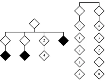
By using a very simple example we could show that the crudeKestimates obtained from genealogies are actu-ally inflated. Figure 4 lists all possible trees of offspring size = 2 with a pedigree generator carrier of the pathologic gene (affected in A, B and C, and non-penetrant heterozy-gous in D, E and F) disclosed by an (impossible) ascertain-ment devoid of any bias. The probabilities associated with each tree are shown in Figure 4.
Let nownA,nB,nC,nD,nE, andnFbe the numbers of structures A, B, C, D, E, and F observed in an ideal, large sample collected without any ascertainment bias. Then, the corresponding likelihood function in logarithmic form would be:
L1= (3nA+2nB+2nD+nE).ln(K) + (nD+nE+nF).ln(1-K) + (nB+2nC+nE+2nF).ln(2-K),
from which the maximum likelihood estimate ofKis ob-tained without difficulties.
A careful collection of a large number of families with offspring number 2 and a tree-generator carrier of the gene would consist only of structures A, B, C and D. Con-figuration E would not be included, as the only affected in-dividual would be, with a large probability, the result of a new mutation; and configuration F would never be
ascer-Table 2- Maximum likelihood estimates of penetrance value (Kij) and
lower (LKij) and upper (UKij) limits of its correspondent 95% credibility
in-terval for all possible configurations obtained from the grouped tree of normal individuals shown in the pedigree of Figure 3.
i j Pij Kij LKij UKij
0 4 0.0625 0.443106 0.149314 0.782835
1 3 0.2500 0.437653 0.147112 0.781286
2 2 0.3750 0.435844 0.146389 0.780826
3 1 0.2500 0.437653 0.147112 0.781286
4 0 0.0625 0.443106 0.149314 0.782835
1.0000 0.437656 0.147116 0.781307
i, j: offspring numbers of the two parents; Pij: normalized product (weighing factor) obtained through Pij= e-22i/i!.e-22j/j!/S(e-22i/i!.e-22j/j!); average estimates for Kij,LKijandUKijare shown in bottom line.
tained, because it contains only normal individuals. The corresponding (logarithmic) likelihood expression would then be given by:
L2= (3nA+2nB+nC+2nD).ln(K) + nD.ln(1-K) + (nB+2nC).ln(2-K),
from which, as in the previous case, the maximum likeli-hood estimate can be easily obtained.
Let us now take the following numerical example. Let the actual (unknown) value of K be 0.8; then the probabili-ties associated with structures A, B, C, D, E, and F would take the values P(A) = 0.128, P(B) = 0.384, P(C) = 0.288, P(D) = 0.032, P(E) = 0.096, and P(F) = 0.288. In a sample of size 1000 we would therefore expect to find the sample numbers nA= 128, nB= 384, nC= 288, nD= 32, nE= 96, and nF= 72. The unbiased estimate would then take the value
K= 0.8, as expected. In the case of an incompletely ascer-tained sample, the biased estimate of K’ would take the value 0.951825 > 0.8.
It is not possible to obtain an exact solution in simple analytical form for the functionK’= f(K), whereK’is the biased maximum likelihood estimate andK the true one (unknown, completely unbiased estimate of the penetrance value), but we can evaluateK’estimates for any given fixed value ofKby means of likelihood expression L2. For any true value ofKthe biased estimate,K’is an inflated value, as we could guess intuitively. Using a program on non-linear regression analysis, such as the NLREG software (Sherrod, 2000), we can adjust the observed set of points to the generalized empirical functiony = axb.ecx(Bronshtein and Semendiaev, 1973) wherey=K’ andx=K.
We then estimated sets of pairs of valuesKandK’
varying offspring size from 2 to 10, and in each case we ob-tained corresponding generalized empirical functions
yi= aixbi.ecix, wherey=K’ andx=K.as in the case of the previous example. The functions corresponding to off-spring sizes from 2 to 10, all showing a perfect statistical fitting with the corresponding observed biased estimates, are plotted in Figure 5, where y stands forK’and x forK. The graph also shows the functionK’ = Kthat corresponds to the case of an offspring with infinite size.
As expected, with sibship size increasing the differ-ence between corresponding estimatesK’ andKbecomes negligible, mainly in relation to values of Kin its usual range (K> 0.8). This is a result that certainly can be gener-alized for any homogeneous or heterogeneous set of
Figure 5- Relation between unbiased (K) and biased (K’) penetrance val-ues, shown at abscissa and ordinate axes respectively, depending on off-spring size (2, 3, 4, 5, 6, ..., infinite).
pedigrees. Since optimizedKestimates are obtained from large filtered pedigrees, or from the pooling of many pedi-grees, the ascertainment bias just discussed will only pro-duce slightly inflatedK estimates. In the case the actual values ofK, as well as the total number of informative indi-viduals (penetrant, obligate non-penetrant and those be-longing to normal trees descending from obligate carriers) are both small, the K estimates will not be reliable, as shown in Figure 5. For offspring sizes of 10 (total of 11 in-formative individuals) or more, it is also easy to conclude that estimated values ofKin the range of 0.5 or more are re-liable and do not need to be corrected. In any case, estimate corrections can be performed by enumerating all possible filtered pedigrees corresponding to a given tree structure and comparing the estimatedKvalues to the inferred actual ones, just as we did before using the very simple examples discussed above.
References
Bronshtein I and Semendiaev K (1973) Manual de Matemáticas para Ingenieros y Estudiantes. 2nd edition. Editorial Mir, Moscow, 694 pp.
Horimoto ARVR, Onodera MT and Otto PA (2010) PENCALC: A program for penetrance estimation in autosomal dominant diseases. Genet Mol Biol 33:455-459.
Lathrop GM, Lalouel JM, Julier C and Ott J (1985) Multilocus linkage analysis in humans: Detection of linkage and esti-mation of recombination. Am J Hum Genet 37:482-498. Majewski F, Küster W, Haar B and Goecke T (1985) Aplasia of
tibia with split-hand/split-foot deformity. Report of six fam-ilies with 35 cases and considerations about variability and penetrance. Hum Genet 70:136-147.
Murphy EA and Chase GA (1975) Principles of Genetic Coun-seling. Year Book Medical Publishers, Chicago, 391 pp. Praxedes LA and Otto PA (2000) Estimation of penetrance from
twin data. Twin Res 3:294-298.
Rogatko A, Pereira CAB and Frota-Pessoa O (1986) A Bayesian method for the estimation of penetrance: application to man-dibulofacial and frontonasal dysostoses. Am J Med Genet 24:231-246.
Internet Resources
Horimoto ARVR (2009) Estimativa do valor da taxa de penetrân-cia em doenças autossômicas dominantes: Estudo teórico de modelos e desenvolvimento de um programa computacional (Penetrance rate estimation in autosomal dominant diseases: theoretical study and development of a computer program). PhD Thesis, Instituto de Biociências, Universidade de São Paulo, São Paulo, 2009. http://www.teses.usp.br/teses/ disponiveis/41/41131/tde-15102009-161545/ (April 16, 2012).
Horimoto ARVR and Otto PA (2008) Penetrance rate estimation. In: Otto PA (ed) Métodos Clásicos y Modernos para el Análisis de Datos en Genética Humana. EdUNaM, Posadas, pp 123-150, http://www.ib.usp.br/~otto/pop_genetics.htm or http://www.lacygh.com.ar/abajo.htm (April 16, 2012). S.A.G.E. (2009) Statistical Analysis from Genetic Epidemiology.
Release 6.0.1, http://darwin.cwru.edu/ (April 16, 2012). Sherrod PH (2000) Non Linear Regression Analysis Program
(NLREG), http://www.nlreg.com/ (April 16, 2012).
Associate Editor: Angela M. Vianna-Morgante
Otto PA, Horimoto ARVR. Penetrance rate estimation in autosomal dominant
conditions. Genetics and Molecular Biology 35(3), 583-588, 2012.
The following text on p. 586 [first paragraph of item 7 (ascertainment issues)], that reads:
Advanced computer programs that perform segregation analysis or estimate linkage, such as the classical S.A.G.E. (S.A.G.E., 2009) and LINKAGE (Lathropet al., 1985) programs we referred to in the introduction section, do not apply any ascertainment bias to the penetrance rate they indirectly estimate.
should be replaced by:
Advanced computer programs that perform segregation analysis or estimate linkage, such as the classical S.A.G.E. (S.A.G.E., 2009) and LINKAGE (Lathropet al., 1985) programs we referred to in the introduction section, do not apply any ascertainment biascorrectionto the penetrance rate they indirectly estimate.
www.sbg.org.br